Article

DaSAM: Disease and Spatial Attention Module-Based Explainable Model for Brain Tumor Detection

by
Sara Tehsin
,
Inzamam Mashood Nasir
,
Robertas Damaševičius
* and
Rytis Maskeliūnas
Centre of Real Time Computer Systems, Kaunas University of Technology, 51368 Kaunas, Lithuania
*
Author to whom correspondence should be addressed.
Big Data Cogn. Comput. 2024, 8(9), 97; https://doi.org/10.3390/bdcc8090097
Submission received: 18 June 2024 / Revised: 3 August 2024 / Accepted: 19 August 2024 / Published: 25 August 2024

Abstract

:
Brain tumors are the result of irregular development of cells. It is a major cause of adult demise worldwide. Several deaths can be avoided with early brain tumor detection. Magnetic resonance imaging (MRI) for earlier brain tumor diagnosis may improve the chance of survival for patients. The most common method of diagnosing brain tumors is MRI. The improved visibility of malignancies in MRI makes therapy easier. The diagnosis and treatment of brain cancers depend on their identification and treatment. Numerous deep learning models are proposed over the last decade including Alexnet, VGG, Inception, ResNet, DenseNet, etc. All these models are trained on a huge dataset, ImageNet. These general models have many parameters, which become irrelevant when implementing these models for a specific problem. This study uses a custom deep-learning model for the classification of brain MRIs. The proposed Disease and Spatial Attention Model (DaSAM) has two modules; (a) the Disease Attention Module (DAM), to distinguish between disease and non-disease regions of an image, and (b) the Spatial Attention Module (SAM), to extract important features. The experiments of the proposed model are conducted on two multi-class datasets that are publicly available, the Figshare and Kaggle datasets, where it achieves precision values of 99% and 96%, respectively. The proposed model is also tested using cross-dataset validation, where it achieved 85% accuracy when trained on the Figshare dataset and validated on the Kaggle dataset. The incorporation of DAM and SAM modules enabled the functionality of feature mapping, which proved to be useful for the highlighting of important features during the decision-making process of the model.

1. Introduction

Tumors in the brain can extensively affect a patient’s quality of life and general existence due to their permanent and catastrophic mental and physical impacts [1]. Brain tumors can be fatal if left untreated [2]. The National Brain Tumor Foundation (NBTF) reports that throughout the last thirty years, the number of people who have passed away from brain tumors has climbed by 300 percent [3]. Many common imaging modalities, such as computed tomography (CT), X-ray, ultrasonography, and magnetic resonance imaging (MRI), are used in medical imaging; they do not, however, show every complex detail and parts of brain tumors. However, they help physicians estimate the tumor’s growth [4]. Brain tumor diagnosis with MRI is a common and very effective procedure [5]. Medical imaging uses magnetic resonance imaging (MRI) to show abnormal bodily tissues. In clinical settings, MRI is becoming more and more common for the diagnosis of brain malignancies [6]. A set of MRI pictures taken at different levels can be used by doctors to determine how the disease is progressing. This method can be time-consuming, though, and it may result in missed or inaccurate diagnoses.
People’s lives have improved because of artificial intelligence (AI) advancements in several sectors, including business, education, and healthcare [7]. Conventional modeling techniques such as decision trees and linear regression offer a meaningful relationship between the model’s outputs and the input data [8]. These models, however less successful, are often called “white-box models”.
Deep learning (DL) is a sub-domain of machine learning that has marked extraordinary achievements in several disciplines, most notably image analysis and recognition [9]. It has been extensively embraced and revolutionized in numerous industries, including healthcare, thanks to its capacity to significantly reduce the amount of human labor required and automate challenging tasks. When it comes to the detection of brain tumors through different image modalities such as MRI, DL has shown promising results in identifying and segmenting lesions accurately, allowing medical professionals to make informed judgments. However, the biggest challenge in using DL for the detection of brain tumors is the black box dilemma. The fact that doctors have voiced concerns about DL’s black box status is not surprising [10]. The complexity of deep learning models due to the highly connected networks of neurons makes it difficult to grasp how they make their predictions. Physicians and researchers have problems because of this lack of interpretability, which makes it difficult for them to accept and confirm the DL system’s outputs and prevents them from comprehending the underlying decision-making process.
Explainable artificial intelligence (XAI) is being considered by researchers as a potential remedy for the “black box” issue [11,12]. XAI aims to fill the gap between the DL model’s complexity and interpretable decision-making needs. It encompasses a variety of methods and techniques meant to provide elucidations and understandings into predictions produced by deep learning models.
This paper proposes a custom convolutional neural network (CNN) with an addition called the Disease and Spatial Attention Model (DaSAM), which has two additional modules: (a) the Disease Attention Module (DAM) to distinguish between disease and non-disease regions of an image and (b) the Spatial Attention Module (SAM) to extract important features to identify and predict brain tumors from a collection of brain MRI images. The proposed DAM and SAM modules enable explainability by mapping important features.
The organization of the rest of the paper is as follows: the literature review is discussed in Section 2; the proposed methodology is discussed in Section 3; experimental results are provided in Section 4 and the conclusion is explained in Section 5.

2. Literature Review

Knowing the type and size of a tumor helps doctors determine which treatment plan is best for each patient. Previous work is categorized into three groups based on the need to develop systems that can analyze medical images and accurately identify areas of the brain that may have tumors or other irregularities: (a) detection systems based on traditional machine learning, (b) deep learning-based detection systems, and (c) systems built on top of pre-trained large architectures. These three methods have been widely used for brain tumor classification. Traditional ML methods were outperformed by DL methods and then pre-trained models were introduced to further enhance the performance of CAD systems. In this study, pre-trained models are taken as inspiration to propose a problem-specific CNN model, shown in Figure 1, which is not only classifying the tumor, but also providing explanations about its predictions. Early detection of brain tumors can lead to more successful treatments with fewer complications or side effects.

2.1. Machine Learning

Numerous research has employed traditional machine learning approaches like support vector machine (SVM), decision tree (DT), k-nearest neighbor (KNN), and adaptive boosting (AdaBoost). The decision tree (DT) model developed by Naik et al. [13] was 96% accurate in classifying brain cancers from CT scan brain pictures. Several researchers have applied a support vector machine (SVM) as a classifier after the extraction of features to identify brain tumors; principal component analysis (PCA) was utilized for dimension reduction and discrete wavelet transform (DWT) was used for the extraction of features by Shil et al. [14], while wavelet transform (WT) was employed for feature extraction by Mathew et al. [15]. A gray-level co-occurrence matrix (GLCM) was employed by Singh and Kaur [16] to extract features, and Amin et al. [17] tried to categorize MRI at the representation and lesion levels. Using k-nearest neighbor (KNN) as a classifier, Ramteke and Monali [18] generated statistical texture feature sets from normal and abnormal images, attaining an 80% accuracy rate.

2.2. Deep Learning

Deep learning systems can identify patterns in scans and identify potential issue areas for more investigation. Compared to preset and manually generated features, deep learning algorithms are more effective in achieving greater results since they automatically extract highly discriminative features in the form of a hierarchy [19,20,21,22,23]. Pereira et al. [24] introduced a novel CNN with deeper architectures and shorter kernels that obtained 89.5% accuracy to automatically predict the grades of LGG and HGG brain tumors on both whole-brain and just tumor area MRI images. For the categorization of brain tumors, CNN was also used in [25,26,27,28]. CNN architecture created by Seetha and Raja [25] had the greatest accuracy rate, at 97.2%. Faster R-CNN was employed as the tumor classifier by Bhanothu et al. [26] and the VGG19 pre-trained model was used for convolution feature map extraction. Their mean precision was 77.6% on average. Das et al. [28] obtained 94.39% accuracy using the proposed CNN design, but Badža and Barjaktarovic [27] proposed a CNN architecture that reached the greatest accuracy of 96.56%. For classifying brain tumors, Afshar et al. [29] suggested modified capsule network designs, or CapsNets, with five possible combinations. They made use of different convolutional layer combinations, convolutional feature maps, different main capsules—both dimensional and non-dimensional—and different numbers of neurons in fully linked layers. Out of all the combinations, the original capsule network had a maximum accuracy of 82.30%, whereas CapsNet with one convolutional layer and 64 feature maps had a highest accuracy of 86.56%.

2.3. Pre-Trained Models

Large datasets are still needed for deep learning models, notwithstanding their recent outstanding classification performance. It has been shown in numerous studies that using pre-trained models increases the efficacy of brain tumor detection. While Khan et al. [30] used VGG16, ResNet50, and InceptionV3 models to identify the type of brain cancers from MRI images, Swati et al. [31] used a feature extractor based on VGG19. In order to classify meningioma, glioma, and pituitary types of brain tumors, Deepak and Ameer [32] developed a classification technique that used deep transfer learning and a pre-trained GoogLeNet architecture to extract features from brain MRI images with five-fold cross-validation. In order to examine the relationship between time and model accuracy, Chelghoum et al. [33] used pre-trained models from ResNet18, ResNet50, ResNet101, ResNet-InceptionV2, AlexNet, VGG16, VGG19, GoogLeNet, and SENet on the same dataset. These models were trained for varied numbers of epochs. A binary classification task of identifying malignant and benign tumors was carried out by Mehrota et al. [34]. The dataset consisted of just 696 T1-weighted MRI images; therefore, they used pre-trained models including SqueezeNet, GoogLeNet, AlexNet, ResNet50, and ResNet101.

2.4. Explainable Artificial Intelligence

While numerous explainable artificial intelligence techniques have already been introduced for image categorization and comprehension tasks, there has not been much focus on explaining brain imaging tasks like segmentation and tumor diagnosis. Two-dimensional Grad-CAM was added to improve the interpretability of the suggested models [35,36,37,38]. Two-dimensional Grad-CAM was utilized by Natekar et al. [35] to interpret Deep Neural Network (DNN) predictions for brain tumor classification. While Esmaeili et al. [36] employed 2D Grad-CAM for performance comparison among DenseNet-121, GoogLeNet, and MobileNet on brain tumor classification, Windisch et al. [37] created heatmaps from 2D GRAD-CAM to show the locations of the brain tumor predicted by the suggested model. Saleem et al. [39] expanded on class activation mapping (CAM) by producing three-dimensional heatmaps that highlight the importance of segmentation data. Zeineldin et al. [40] implemented seven state-of-the-art explanation methods to present a novel framework (NeuroXAI) for viewing deep learning networks. Using NeuroXAI, they classified and segmented brain cancers using the magnetic resonance (MR) modality.

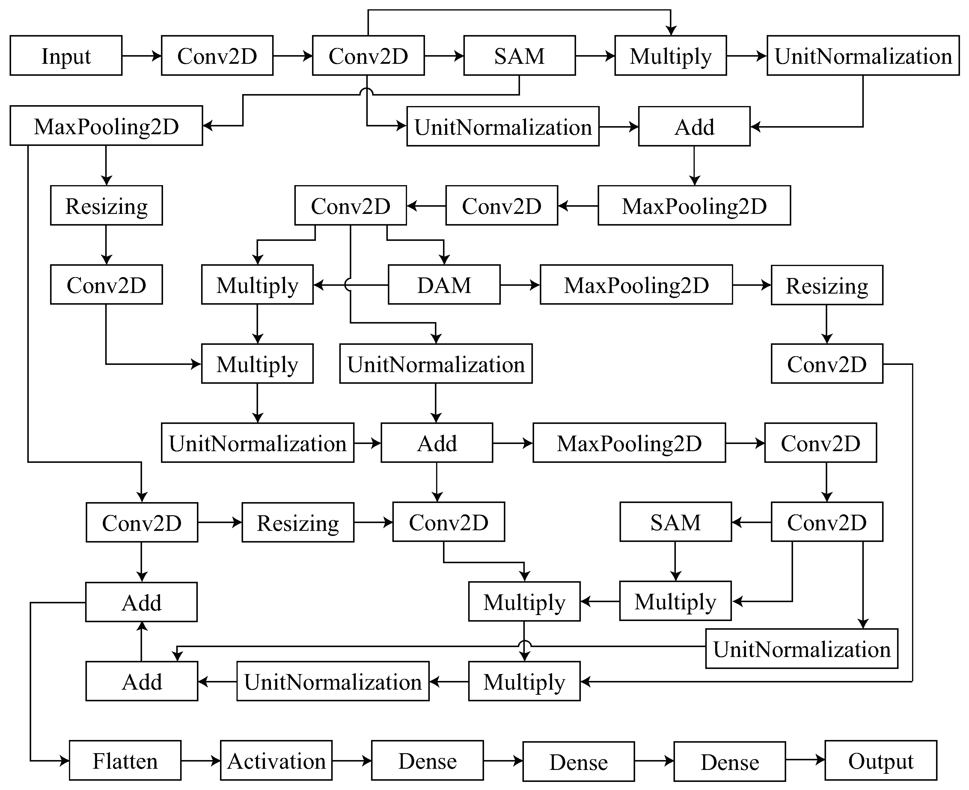
3. Proposed Methodology

This section provides a comprehensive explanation of the proposed Disease and Spatial Attention Model (DaSAM). Figure 1 illustrates the framework of the proposed model. The DaSAM has two modules: (a) the Disease Attention Module (DAM) and (b) the Spatial Attention Module (SAM). The proposed CNN framework incorporates SAM at the beginning and end to extract important features, while DAM is incorporated in the middle to distinguish between disease and non-disease regions of an image. The input image contains significant and distinctive information for brain tumor detection, both in terms of its spatial and temporal aspects. Nevertheless, the data’s distribution is often imbalanced. Not all elements of the image are directly linked to the disease in terms of their spatial relationship. Consequently, it is typical to allocate different levels of attention to different parts of the image. These findings resulted in the formulation of a DAM and SAM that can accurately identify the most important section of an image and extract key features.

3.1. Disease Attention Module

Each feature in an input image has a distinct impact on the classification of a brain tumor. Tumors can occur in connected and/or concentrated regions or they can appear in multiple regions. Hence, it is important to note that not all features hold significance in the classification of cancer. Additionally, there exist certain features that have less relevance or no relevance whatsoever to the specific category being targeted. These irrelevant features, when fed to a CNN model, are treated as noise, which can lead to inaccurate recognition results. On the other hand, certain features are more significant for the targeted classes and require greater attention. CNNs designed specifically for brain tumor exhibit greater reliability when they focus on shorter yet more information-dense segments of the image, as opposed to analyzing the entire image. This study proposes a DAM which compresses the spatial and channel dimensions of the input feature map to focus on the temporal dimension and extract these features. These features are then used to generate temporal descriptors, which can aggregate the features that are relevant to specific cancerous regions. The DAM also generates disease attention scores based on this aggregation. The output feature map of the convolution layer is obtained by translating the original input feature vector to F j = x 1 , , x j , as depicted in Figure 2.
The feature map is divided into two separate feature descriptors, A v g j F 1 × 1 × 1 × J and M a x j F 1 × 1 × 1 × J , which are used to represent the attention weights of the input image. The sizes of both channel and spatial dimensions are simultaneously reduced by applying a v g p o o l and m a x p o o l operations. The original features are further processed to generate the disease attention maps A v g j and M a x j . The entire procedure is as follows:
A v g j = a v g p o o l x j = 1 W × H × C w = 1 W h = 1 H c = 1 C F w × h × c × J
M a x j = m a x p o o l x j = m a x x j
The variables M a x j and A v g j represent the local and global features of the image, respectively. The variables w and h show the indices of the spatial domain, whereas c is the indices of the channel part. j is an indicator of temporal features that range from 1 to J. W, H, and C show the width, height, and channel of the feature map, respectively. The module combines two distinct temporal feature descriptors by summing their elements to generate the final temporal features T f , which has dimensions of F 1 × 1 × 1 × J operates as follows:
T f = M a x j + A v g j
After this, the output of the convolution layer is forwarded to the reshape layer, which transforms it into the original shape, and a concatenate layer aggregates the output of the reshape layer. At the end, a fully connected (FC) layer is integrated, which has a sigmoid function to obtain the weights as follows:
ρ D A M = δ c o n v T f
Here, conv is a convolution layer and δ represents a sigmoid function, which generates an output ρ D A M in range [0, , 1].

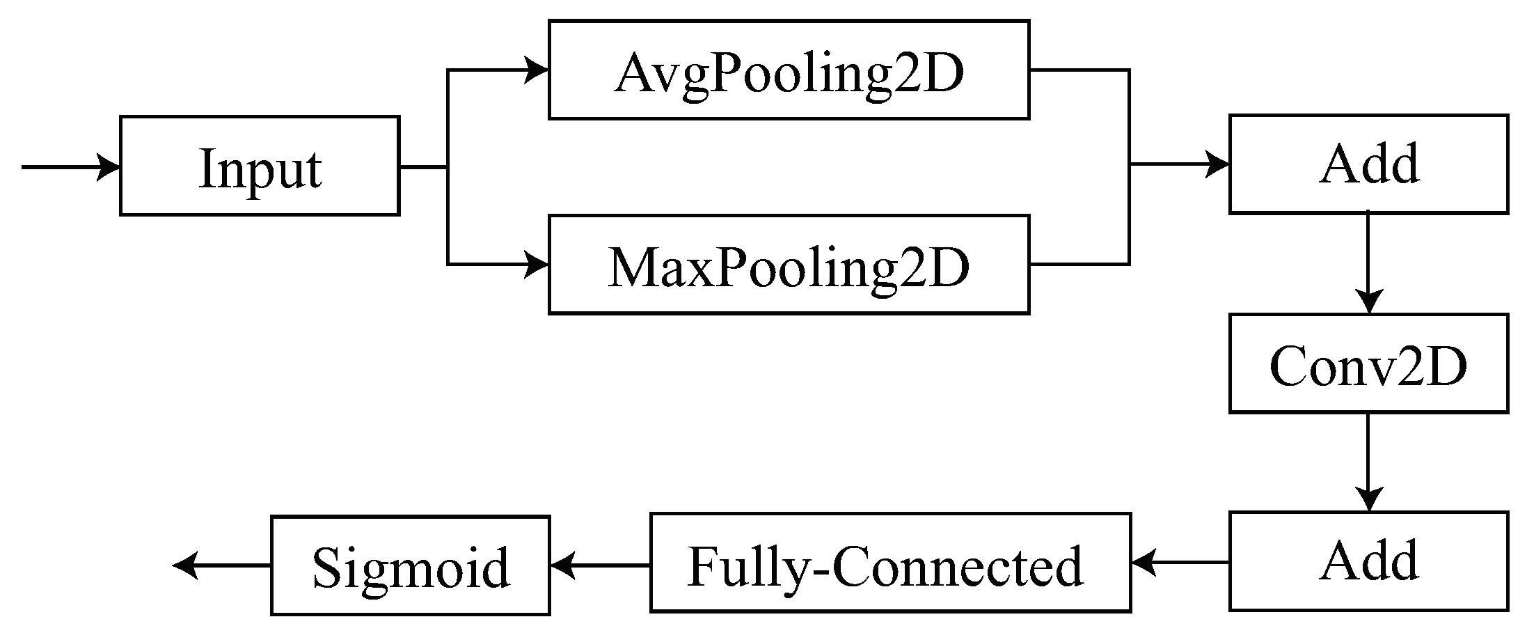
3.2. Spatial Attention Module

The study also investigates spatial attention at the channel level, which aids in the identification of unique features for the detection of brain tumors. The individual channels of a CNN-based model can be considered as spatial representations of the cancer class. Hence, SAM is specifically designed to acquire the significance score of each channel of a CNN that correlates to a given tumor characteristic. The model emphasizes spatial regions with high scores corresponding to a certain class, while discarding regions with low values deemed unimportant. After undergoing specific processing, the output feature map obtained from the DAM is inputted into the SAM. The SAM efficiently reduces the size of the feature map in both the spatial and temporal dimensions to retrieve channel information. This compression technique also enables the retrieval of channel descriptors, which are utilized to capture spatial attention maps effectively. Figure 3 illustrates how the global average pool and global maximum pool layers merge the spatial and temporal aspects of the input image and produce attention feature maps.
As channel information shows the spatial characteristics, the dimension of the channel is preserved, resulting in the generation of two distinct channel descriptions, namely m a x k and A v g k . The spatial attention feature descriptor can be derived using the following formula:
ρ S A M = δ τ 1 τ 2 A v g k + τ 1 τ 2 m a x k × φ
The symbol δ represents the sigmoid function, which guarantees a feature maps descriptor in a range between 0 and 1. τ 1 and τ 2 are trainable parameters, while φ denotes the reduction ratio. m a x k and A v g k are two descriptors, where A v g k quantifies the overall background information for each channel, and m a x k quantifies the specific discriminant information at a local level.

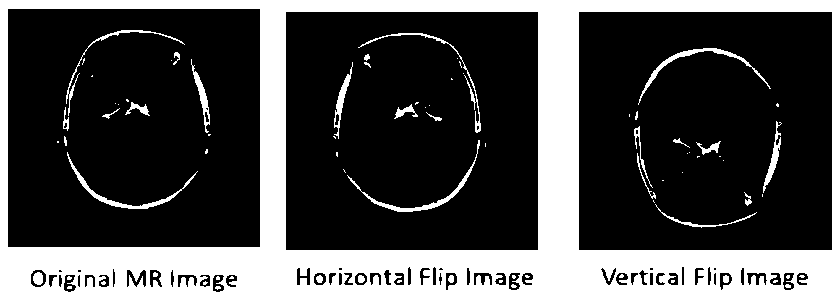
3.3. Data Preprocessing and Augmentation

The input size of the training and testing images was 128 × 128 . The images were resized to the standard size. The proposed model obtained an RGB image, so the grayscale conversion was not performed in the preprocessing step. A training, validation, and test ratio of 60-10-30 was used for the Kaggle dataset and a ratio of 80-10-10 was used for the Figshare dataset throughout our experimentation. The validation step was performed to avoid overfitting and evaluating the model. After the preprocessing step, data augmentation was performed to increase the training images and train the model to diverse types of data. Horizontal and vertical flips were used to normalize the datasets in this step. Figure 4 shows the horizontal and vertical flips of the training images.

4. Experimental Results

The model’s training and testing requirements regarding hardware and software will be discussed in this section. During the model’s evaluation, the analysis of the parameters and the model will be conducted. All experiments have been run on Google Colaboratory, which is an open-source platform that offers resources for academic and research tasks. TensorFlow and Keras API libraries were utilized for development, and four GPUs with 16 GB RAM were employed.

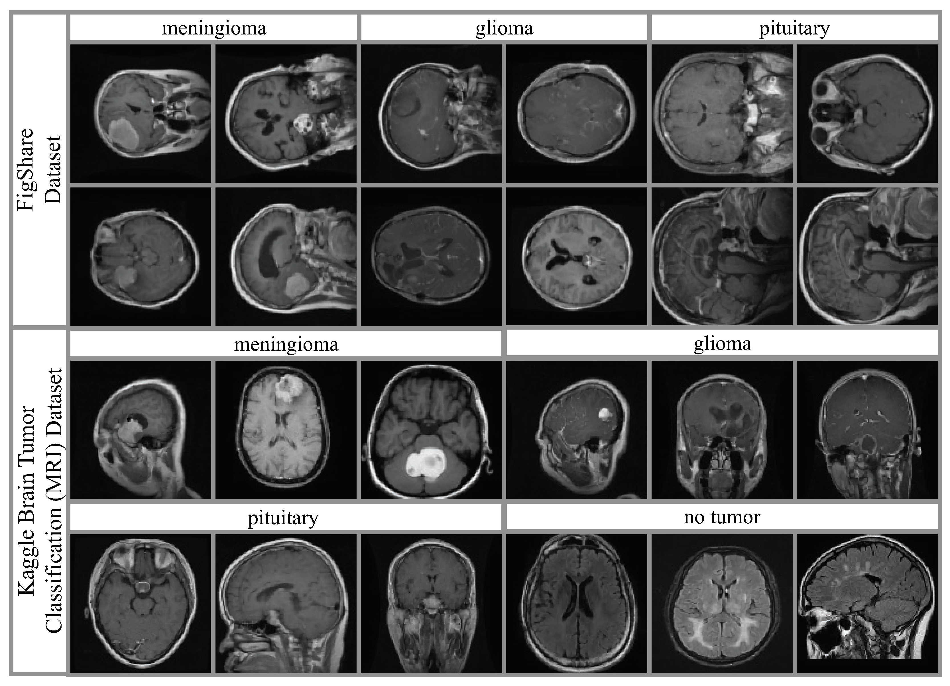
4.1. Datasets and Hyperparameter Settings

Extensive experiments have been conducted to check the proposed model’s efficiency. Two publicly available datasets are used for the experimental purpose. One dataset is publicly available: Kaggle Brain Tumor Classification (MRI) [41], which is a multi-class brain tumor dataset having four classes which include no tumor (N), glioma (G), meningioma (M), and pituitary (P). The other dataset one is the Figshare brain tumor dataset [42], which has three classes: glioma (G), meningioma (M), and pituitary (P). Sample images from these two datasets are shown in Figure 5.
The proposed model is trained effectively by fine-tuning hyperparameters such as batch size, learning rate, optimizer, epoch, and loss function. Categorical cross-entropy has been employed as the loss function for the multi-class tumor problem classification. The details of the hyperparameters are given in Table 1.

4.2. Classification Results

The classification results of the proposed model utilizing the testing data are presented in Table 2. The performance measures are precision (P), recall (R), F1 score (F), and accuracy (A). The proposed model accurately classifies different types of tumors, such as meningioma, glioma, and pituitary, with high precision rates. Specifically, it achieves precision values of 97% for meningioma, 100% for glioma, and 99% for pituitary on the Figshare dataset. Additionally, it achieves precision values of 92% for meningioma, 98% for glioma, 93% for pituitary, and 94% for no tumor when applied to Kaggle dataset. These results demonstrate the effectiveness of our model using publicly available datasets.
The visual results of the proposed model on the Figshare dataset are illustrated in Figure 6. This figure displays the input image, the ground truth image, and the predicted attention of the proposed model. The incorporation of SAM and DAM modules in the proposed CNN architecture accurately maps the tumor component of the input image. Nevertheless, the model encounters confusion when predicting the two samples displayed in the last row. In one case, it incorrectly associates a smaller area, while in the other case, it incorrectly associates an additional area. This misprediction is due to the visual resemblance with other classes.
Cross-dataset validation is also performed to check the validity of the proposed model. The Figshare dataset has three classes, while the Kaggle dataset has four classes. The extra class, no tumor, was removed class from the Kaggle dataset, and then the proposed model was tested by training on the Figshare dataset and testing on the Kaggle dataset. The performance of the proposed model is given in Table 3.
The visual results are shown in Figure 7, where the images of the Kaggle dataset are given and the proposed model highlights the maps important regions of the tumor. However, there are no ground truth images given for the Kaggle dataset and thus its validity cannot be established.

4.3. Ablation Analysis

An ablation study was conducted by varying the learning rate, the optimizer, and split ratio. All experiments were conducted on the Figshare and Kaggle datasets. It has been noted through experimentation that the best results are attained once the learning rate is 0.01 on both datasets. The Adam optimizer is most suitable for both datasets as provides good model convergence when compared to the other optimizers. In the case of the Figshare dataset, an 80-10-10 split ratio provides better results and for the Kaggle dataset a 60-10-30 split ratio provides prominent results. The results of varying the learning rate, the optimizer, and split ratio are given in Table 4.
Figure 8 illustrates the impact of different learning rates on the performance metrics for Figshare and Kaggle datasets. Cross-dataset validation tests a model’s robustness across several datasets. This improves model generalization, avoids overfitting, and handles data variability. It identifies biases and tests whether the model can perform consistently across data characteristics, noise, and feature distributions. This technique finds solid, dependable models for varied real-world applications. Varying learning rates have distinct impacts on model performance for the Figshare and Kaggle datasets. At a high learning rate (0.01), Figshare shows excellent performance across all metrics (P, R, F at 98%, A at 99%), indicating quick and effective convergence, while Kaggle performs slightly lower (P at 95%, R at 96%, F at 94%, A at 96%). At a moderate learning rate (0.001), Figshare experiences a slight drop but maintains good performance (P at 92%, R at 94%, F at 95%, A at 96%), whereas Kaggle sees a more noticeable decline (P at 92%, R at 90%, F at 93%, A at 91%). With a low learning rate (0.0001), Figshare remains stable (P at 93%, R at 95%, F at 93%, A at 92%), but Kaggle shows further degradation (P at 91%, R at 88%, F at 90%, A at 89%). At a very low learning rate (0.00001), Figshare’s metrics recover somewhat (P at 91%, R at 97%, F at 94%, A at 93%), particularly in recall, while Kaggle sees slight improvement in recall (92%) and F1 score (93%) but remains lower in precision (90%) and accuracy (95%), indicating some instability at very low learning rates.
Figure 9 the results for different optimizers on the Figshare and Kaggle datasets. Each plot displays the metrics for precision (P), recall (R), F1 score (F), and accuracy (A) across various optimizers (SGD, RMSprop, Adam, Adadelta). The performance of each optimizer is compared, showing how they impact the model’s effectiveness in terms of these metrics for both datasets. The results reveal several interesting trends and observations across different optimizers for the Figshare and Kaggle datasets. Notably, the Adam optimizer consistently achieves the highest performance metrics on both datasets, with precision, recall, and F1 score values of 98% and an accuracy of 99% for Figshare, and slightly lower but still leading values for Kaggle. This indicates Adam’s superior capability in handling diverse data distributions. Conversely, SGD and Adadelta show significantly lower performance, particularly for the Kaggle dataset, where their metrics hover around 80%. RMSprop performs moderately well, but still trails behind Adam, especially in recall and accuracy. The most intriguing trend is the stark contrast in optimizer effectiveness, highlighting Adam’s robustness and efficiency in optimizing complex models, while traditional optimizers like SGD struggle to achieve comparable results, especially on more challenging datasets like Kaggle.
The results of the different split ratios reveal several key insights into model performance for the Figshare and Kaggle datasets. For Figshare, the 80-10-10 split yields the highest performance across all metrics, with precision, recall, F1 score, and accuracy all around 98–99%, indicating that a larger training set significantly enhances model effectiveness. Interestingly, the 60-10-30 split also performs well, particularly in precision and accuracy (81% and 84% respectively), suggesting a good balance between training and testing data. Conversely, the 50-25-25 split shows the lowest performance, especially in F1 score (63%) and accuracy (67%), highlighting the limitations of smaller training sets. For the Kaggle dataset, the 60-10-30 split provides the best overall results, with precision at 95%, recall at 96%, F1 score at 94%, and accuracy at 96%, demonstrating optimal performance with this balanced split. However, the 80-10-10 split shows a slight decrease in precision and F1 score (91% and 92% respectively), indicating that while a larger training set improves recall and accuracy, it may slightly impact other metrics. The 50-25-25 split again shows the lowest performance, particularly in F1 score (80%) and accuracy (85%), reinforcing the importance of an adequate training set size for robust model performance (see Figure 10).
Following the completion of the validation of the proposed model, a comprehensive comparison is carried out. An overview of the comparison is provided in Table 5 for both selected publicly available datasets.

5. Conclusions

Tumors pose a significant threat to human health, as malignant cells can invade adjacent tissue and metastasize to distant sites within the body. The need for early detection of brain tumors to administer appropriate medical intervention has been well acknowledged. This study presents DaSAM, a system designed to detect brain cancers using MRI data. The Kaggle dataset was used to evaluate the performance of DaSAM in multi-class classification. The dataset consists of four types of tumor images. The Figshare dataset was also used, which has three types of tumor images. The achieved results show that the proposed methodology can highlight the important features by using its DAM and SAM modules.
The study also demonstrates the critical role of hyperparameter tuning in deep learning models, particularly for medical image analysis. The Adam optimizer, coupled with an appropriately high learning rate and a balanced split ratio, consistently enhances model performance. These insights can guide future research and practical applications in brain tumor detection, emphasizing the need for careful optimization of learning parameters to achieve the best results.
In the future, the focus will be on the development of models that are interpretable and capable of accurately assessing tumor segmentation for precise tumor localization. The proposed model is trained and tested on a custom CNN model, involving modules like DAM and SAM. A famous explainable model, KAN, can also be implemented and compared with the proposed model, which can improve its validity.

Author Contributions

Conceptualization, S.T., I.M.N., R.D. and R.M.; methodology, S.T., I.M.N., R.D. and R.M.; software, S.T. and I.M.N.; validation, S.T., I.M.N., R.D. and R.M.; formal analysis, S.T., I.M.N., R.D. and R.M.; investigation, S.T., I.M.N., R.D. and R.M.; writing—original draft preparation, S.T. and I.M.N.; writing—review and editing, R.D. and R.M.; visualization, S.T. and I.M.N.; supervision, R.D.; funding acquisition, R.D. All authors have read and agreed to the published version of the manuscript.

Funding

This research received no external funding.

Institutional Review Board Statement

Not applicable.

Informed Consent Statement

Not applicable.

Data Availability Statement

This study used two publicly available datasets. The Brain Tumor Classification dataset is available at https://www.kaggle.com/datasets/sartajbhuvaji/brain-tumor-classification-mri, accessed on 1 March 2024. The Figshare brain tumor dataset is available at https://figshare.com/articles/dataset/brain-tumor-dataset/1512427, accessed on 1 March 2024.

Conflicts of Interest

The authors declare no conflicts of interest.

References

  1. Mustaqeem, A.; Javed, A.; Fatima, T. An Efficient Brain Tumor Detection Algorithm Using Watershed & Thresholding Based Segmentation. Int. J. Image Graph. Signal Process. 2012, 4, 34–39. [Google Scholar]
  2. Meng, Y.; Tang, C.; Yu, J.; Meng, S.; Zhang, W. Exposure to lead increases the risk of meningioma and brain cancer: A meta-analysis. J. Trace Elem. Med. Biol. 2020, 60, 126474. [Google Scholar] [CrossRef] [PubMed]
  3. El-Dahshan, E.-S.A.; Mohsen, H.M.; Revett, K.; Salem, A.-B.M. Computer-aided diagnosis of human brain tumor through MRI: A survey and a new algorithm. Expert Syst. Appl. 2014, 41, 5526–5545. [Google Scholar] [CrossRef]
  4. Liu, J.; Li, M.; Wang, J.; Wu, F.; Liu, T.; Pan, Y. A Survey of MRI-Based Brain Tumor Segmentation Methods. Tsinghua Sci. Technol. 2014, 19, 578–595. [Google Scholar]
  5. Maqsood, S.; Damasevicius, R.; Shah, F.M. An Efficient Approach for the Detection of Brain Tumor Using Fuzzy Logic and U-NET CNN Classification. In Lecture Notes in Computer Science (Including Subseries Lecture Notes in Artificial Intelligence and Lecture Notes in Bioinformatics); Springer: Berlin/Heidelberg, Germany, 2021; Volume 12953 LNCS, pp. 105–118. [Google Scholar] [CrossRef]
  6. Wen, P.Y.; Macdonald, D.R.; Reardon, D.A.; Cloughesy, T.F.; Sorensen, A.G.; Galanis, E.; Degroot, J.; Wick, W.; Gilbert, M.R.; Lassman, A.B.; et al. Updated response assessment criteria for high-grade gliomas: Response assessment in neuro-oncology working group. J. Clin. Oncol. 2010, 28, 1963–1972. [Google Scholar] [CrossRef] [PubMed]
  7. Battineni, G.; Sagaro, G.G.; Chinatalapudi, N.; Amenta, F. Applications of Machine Learning Predictive Models in the Chronic Disease Diagnosis. J. Pers. Med. 2020, 10, 21. [Google Scholar] [CrossRef] [PubMed]
  8. Topol, E.J. High-performance medicine: The convergence of human and artificial intelligence. Nat. Med. 2019, 25, 44–56. [Google Scholar] [CrossRef] [PubMed]
  9. Zuo, C.; Qian, J.; Feng, S.; Yin, W.; Li, Y.; Fan, P.; Han, J.; Qian, K.; Chen, Q. Deep learning in optical metrology: A review. Light Sci. Appl. 2022, 11, 39. [Google Scholar] [CrossRef] [PubMed]
  10. Jia, X.; Ren, L.; Cai, J. Clinical implementation of AI technologies will require interpretable AI models. Med. Phys. 2020, 47, 1–4. [Google Scholar] [CrossRef]
  11. Zhang, Y.; Weng, Y.; Lund, J. Applications of Explainable Artificial Intelligence in Diagnosis and Surgery. Diagnostics 2022, 12, 237. [Google Scholar] [CrossRef]
  12. Hassija, V.; Chamola, V.; Mahapatra, A.; Singal, A.; Goel, D.; Huang, K.; Scardapane, S.; Spinelli, I.; Mahmud, M.; Hussain, A. Interpreting Black-Box Models: A Review on Explainable Artificial Intelligence. Cognit. Comput. 2023, 16, 45–74. [Google Scholar] [CrossRef]
  13. Naik, J.; Patel, S. Tumor detection and classification using decision tree in brain MRI. Int. J. Comput. Sci. Netw. Secur. 2014, 14, 87. [Google Scholar]
  14. Shil, S.; Polly, F.; Hossain, M.A.; Ifthekhar, M.S.; Uddin, M.N.; Jang, Y.M. An improved brain tumor detection and classification mechanism. In Proceedings of the 2017 International Conference on Information and Communication Technology Convergence (ICTC), Jeju, Republic of Korea, 18–20 October 2017; pp. 54–57. [Google Scholar]
  15. Mathew, A.R.; Anto, P.B. Tumor detection and classification of MRI brain image using wavelet transform and SVM. In Proceedings of the IEEE 2017 International Conference on Signal Processing and Communication (ICSPC), Coimbatore, India, 28–29 July 2017; pp. 75–78. [Google Scholar]
  16. Singh, D.; Kaur, K. Classification of abnormalities in brain MRI images using GLCM, PCA and SVM. Int. J. Eng. Adv. Technol. 2012, 1, 243–248. [Google Scholar]
  17. Amin, J.; Sharif, M.; Yasmin, M.; Fernandes, S.L. A distinctive approach in brain tumor detection and classification using MRI. Pattern Recognit. Lett. 2020, 139, 118–127. [Google Scholar] [CrossRef]
  18. Ramteke, R.; Monali, Y.K. Automatic medical image classification and abnormality detection using K-Nearest Neighbour. Int. J. Adv. Comput. Res. 2012, 2, 190–196. [Google Scholar]
  19. Rajinikanth, V.; Kadry, S.; Nam, Y. Convolutional-Neural-Network Assisted Segmentation and SVM Classification of Brain Tumor in Clinical MRI Slices. Inf. Tech. Control 2021, 50, 342–356. [Google Scholar] [CrossRef]
  20. Kurdi, S.Z.; Ali, M.H.; Jaber, M.M.; Saba, T.; Rehman, A.; Damaševičius, R. Brain Tumor Classification Using Meta-Heuristic Optimized Convolutional Neural Networks. J. Pers. Med. 2023, 13, 181. [Google Scholar] [CrossRef] [PubMed]
  21. Khan, M.; Khan, A.; Alhaisoni, M.; Alqahtani, A.; Alsubai, S.; Alharbi, M.; Malik, N.; Damaševičius, R. Multimodal brain tumor detection and classification using deep saliency map and improved dragonfly optimization algorithm. Int. J. Imaging Syst. Technol. 2023, 33, 572–587. [Google Scholar] [CrossRef]
  22. Badjie, B.; Ülker, E.D. A Deep Transfer Learning Based Architecture for Brain Tumor Classification Using MR Images. Inform. Tech. Control 2022, 51, 332–344. [Google Scholar] [CrossRef]
  23. Zheng, Q.; Saponara, S.; Tian, X.; Yu, Z.; Elhanashi, A.; Yu, R. A real-time constellation image classification method of wireless communication signals based on the lightweight network MobileViT. Cogn. Neurodynamics 2024, 18, 659–671. [Google Scholar] [CrossRef]
  24. Pereira, S.; Meier, R.; Alves, V.; Reyes, M.; Silva, C.A. Automatic brain tumor grading from MRI data using convolutional neural networks and quality assessment. In Understanding and Interpreting Machine Learning in Medical Image Computing Applications; Springer: Cham, Switzerland, 2018; pp. 106–114. [Google Scholar]
  25. Seetha, J.; Raja, S. Brain tumor classification using convolutional neural networks. Biomed. Pharmacol. J. 2018, 11, 1457–1461. [Google Scholar] [CrossRef]
  26. Bhanothu, Y.; Kamalakannan, A.; Rajamanickam, G. Detection and classification of brain tumor in MRI images using deep convolutional network. In Proceedings of the 2020 6th International Conference on Advanced Computing and Communication Systems (ICACCS), Coimbatore, India, 6–7 March 2020; pp. 248–252. [Google Scholar]
  27. Badža, M.M.; Barjaktarović, M.Č. Classification of brain tumors from mri images using a convolutional neural network. Appl. Sci. 2020, 10, 1999. [Google Scholar] [CrossRef]
  28. Das, S.; Aranya, O.R.R.; Labiba, N.N. Brain Tumor Classification Using Convolutional Neural Network. In Proceedings of the 2019 1st International Conference on Advances in Science, Engineering and Robotics Technology (ICASERT), Dhaka, Bangladesh, 3–5 May 2019; pp. 1–5. [Google Scholar]
  29. Afshar, P.; Mohammadi, A.; Plataniotis, K.N. Brain Tumor Type Classification via Capsule Networks. In Proceedings of the 2018 25th IEEE International Conference on Image Processing (ICIP), Athens, Greece, 7–10 October 2018; pp. 3129–3133. [Google Scholar]
  30. Khan, H.A.; Jue, W.; Mushtaq, M.; Mushtaq, M.U. Brain tumor classification in MRI image using convolutional neural network. Math. Biosci. Eng. 2020, 17, 6203–6216. [Google Scholar] [CrossRef]
  31. Swati, Z.N.K.; Zhao, Q.; Kabir, M.; Ali, F.; Ali, Z.; Ahmed, S.; Lu, J. Contentbased brain tumor retrieval for mr images using transfer learning. IEEE Access 2019, 7, 809–817. [Google Scholar] [CrossRef]
  32. Deepak, S.; Ameer, P.M. Brain Tumor Classification using Deep CNN features via transfer learning. Comput. Biol. Med. 2019, 111, 103345. [Google Scholar] [CrossRef] [PubMed]
  33. Chelghoum, R.; Ikhlef, A.; Hameurlaine, A.; Jacquir, S. Transfer learning using convolutional neural network architectures for brain tumor classification from MRI images. In Proceedings of the IFIP International Conference on Artificial Intelligence Applications and Innovations, Neos Marmaras, Greece, 5–7 June 2020; pp. 189–200. [Google Scholar]
  34. Mehrotra, R.; Ansari, M.A.; Agrawal, R.; Anand, R.S. A transfer learning approach for AI-based classification of brain tumors. Mach. Learn. Appl. 2020, 2, 100003. [Google Scholar] [CrossRef]
  35. Natekar, P.; Kori, A.; Krishnamurthi, G. Demystifying brain tumor segmentation networks: Interpretability and uncertainty analysis. Front. Comput. Neurosci. 2020, 14, 6. [Google Scholar] [CrossRef]
  36. Esmaeili, M.; Vettukattil, R.; Banitalebi, H.; Krogh, N.R.; Geitung, J.T. Explainable artificial intelligence for human-machine interaction in brain tumor localization. J. Pers. Med. 2021, 11, 1213. [Google Scholar] [CrossRef]
  37. Windisch, P.; Weber, P.; Fürweger, C.; Ehret, F.; Kufeld, M.; Zwahlen, D.; Muacevic, A. Implementation of model explainability for a basic brain tumor detection using convolutional neural networks on MRI slices. Neuroradiology 2020, 62, 1515–1518. [Google Scholar] [CrossRef] [PubMed]
  38. Pikulkaew, K. Enhancing Brain Tumor Detection with Gradient-Weighted Class Activation Mapping and Deep Learning Techniques. In Proceedings of the 2023 20th International Joint Conference on Computer Science and Software Engineering (JCSSE), Phitsanulok, Thailand, 28 June 2023; pp. 339–344. [Google Scholar]
  39. Saleem, H.; Shahid, A.R.; Raza, B. Visual interpretability in 3D brain tumor segmentation network. Comput. Biol. Med. 2021, 133, 104410. [Google Scholar] [CrossRef]
  40. Zeineldin, R.A.; Karar, M.E.; Elshaer, Z.; Coburger, J.; Wirtz, C.R.; Burgert, O.; Mathis-Ullrich, F. Explainability of deep neural networks for MRI analysis of brain tumors. Int. J. Comput. Assist. Radiol. Surg. 2022, 17, 1673–1683. [Google Scholar] [CrossRef] [PubMed]
  41. Brain Tumor Classification (MRI). Available online: https://www.kaggle.com/datasets/sartajbhuvaji/brain-tumor-classification-mri (accessed on 1 March 2024).
  42. Figshare Brain Tumor Dataset. Available online: https://figshare.com/articles/dataset/brain-tumor-dataset/1512427 (accessed on 1 March 2024).
  43. Lamrani, D.; Cherradi, B.; El Gannour, O.; Bouqentar, M.A.; Bahatti, L. Brain tumor detection using MRI images and convolutional neural network. Int. J. Adv. Comput. Sci. Appl. 2022, 13, 452–460. [Google Scholar] [CrossRef]
  44. Minarno, A.E.; Mandiri, M.H.C.; Munarko, Y.; Hariyady, H. Convolutional neural network with hyperparameter tuning for brain tumor classification. Kinetik Game Technol. Inf. Syst. Comput. Netw. Comput. Electron. Control 2021, 6, 127–132. [Google Scholar]
  45. Saxena, P.; Maheshwari, A.; Maheshwari, S. Predictive modeling of brain tumor: A Deep learning approach. In Innovations in Computational Intelligence and Computer Vision; Springer: Singapore, 2021; pp. 275–285. [Google Scholar]
  46. Rahman, T.; Islam, M.S. MRI brain tumor classification using deep convolutional neural network. In Proceedings of the 2022 3rd International Conference on Innovations in Science, Engineering and Technology (ICISET), Chittagong, Bangladesh, 26–27 February 2022; pp. 451–456. [Google Scholar]
  47. Rahman, T.; Islam, M.S. MRI brain tumor detection and classification using parallel deep convolutional neural networks. Meas. Sens. 2023, 26, 100694. [Google Scholar] [CrossRef]
Figure 1. The proposed model’s architecture with integrated SAMs and DAMs.
Bdcc 08 00097 g001
Figure 2. The proposed DAM’s architecture.
Bdcc 08 00097 g002
Figure 3. The proposed SAM’s architecture.
Bdcc 08 00097 g003
Figure 4. The output of data augmentation operations, i.e., horizontal and vertical flips.
Bdcc 08 00097 g004
Figure 5. Sample images from Figshare and Kaggle datasets.
Bdcc 08 00097 g005
Figure 6. Visual results of the proposed model on the Figshare dataset.
Bdcc 08 00097 g006
Figure 7. The visualized maps of the proposed model when trained on the Figshare dataset and evaluated on the Kaggle dataset.
Bdcc 08 00097 g007
Figure 8. Influence of learning rate hyperparameter on performance of classification in Figshare and Kaggle datasets.
Bdcc 08 00097 g008
Figure 9. Performance results for different optimizers on the Figshare and Kaggle datasets.
Bdcc 08 00097 g009
Figure 10. Performance results of different split ratios on Figshare and Kaggle datasets.
Bdcc 08 00097 g010
Table 1. Hyperparameters and their values.
ParametersValue
Epochs100
Batch Size32
Epsilon0.1
OptimizerAdam
Learning Rate0.01
Initial Class WeightsFigshare: 0: 1.44, 1: 0.72, 2: 1.09
Kaggle: 0: 0.37, 1: 0.85, 2: 1.37, 3: 1.98
Early StoppingMonitor = Validation Loss, Patience = 20, Minimum Change = 0.001
Table 2. Performance of the proposed model on testing data. Here: P—Precision, R—Recall, F—F-score, A—Accuracy.
ClassFigshare DatasetKaggle Dataset
P (%)R (%)F (%)A (%)P (%)R (%)F (%)A (%)
M97100979992979596
G1009698989496
P9910099939794
N---949495
Macro Average989998959794
Weighted Average989898959694
Table 3. Cross-dataset validation results when trained on Figshare and tested on Kaggle datasets.
ClassesP (%)R (%)F (%)A (%)
M83808585
G808179
P788583
Macro Average818382
Weighted Average808184
Table 4. Classification results with different hyperparameter values on the Figshare and Kaggle datasets.
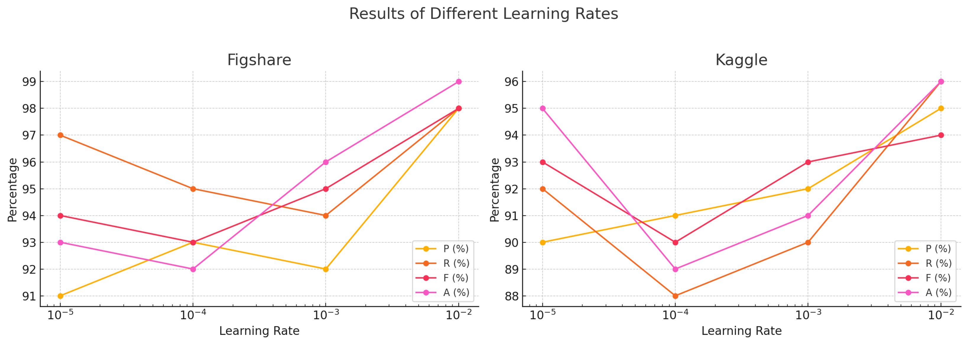
Results of Different Learning Rates
Learning RateFigshareKaggle
P (%)R (%)F (%)A (%)P (%)R (%)F (%)A (%)
0.019898989995969496
0.0019294959692909391
0.00019395939291889089
0.000019197949390929395
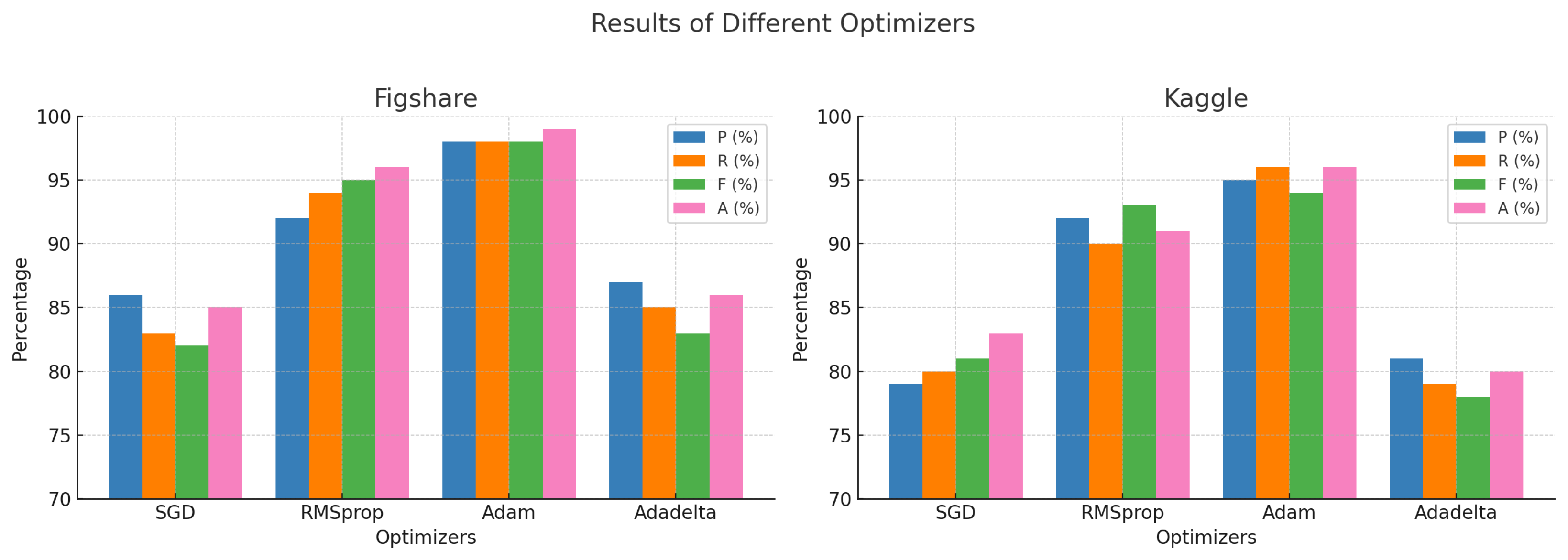
Results of Different Optimizers
OptimizersFigshareKaggle
P (%R (%)F (%)A (%)P (%)R (%)F (%)A (%)
SGD8683828579808183
RMSprop9294959692909391
Adam9898989995969496
Adadelta8785838681797880
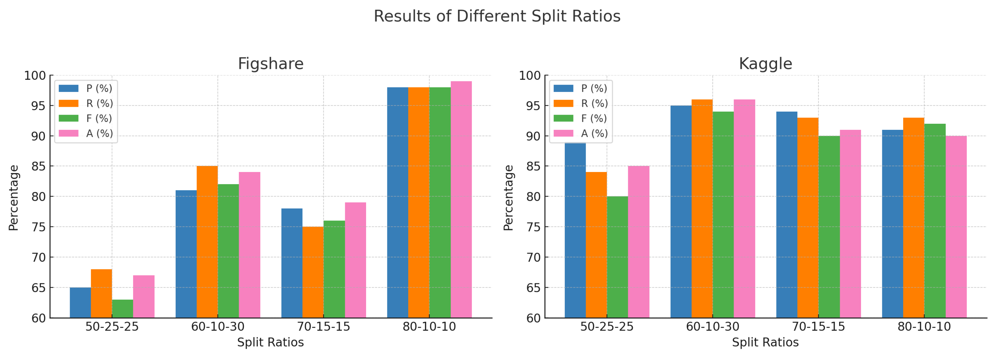
Results of Different Split Ratio
Split RatioFigshareKaggle
P (%)R (%)F (%)A (%)P (%)R (%)F (%)A (%)
50-25-256568636789848085
60-10-308185828495969496
70-15-157875767994939091
80-10-109898989991939290
Table 5. Comparison with exiting techniques.
ModelDatasetAccuracy
CNN [43]Figshare96%
Binary Dataset94%
CNN with Pre-processing [44]Kaggle Dataset96%
Transfer learning-based CNN [45]Figshare94%
Binary Dataset95%
CNN with Pre-processing [46]Figshare96%
Kaggle Dataset94%
CNN with Pre-processing [47]Figshare98%
Kaggle Dataset98%
Proposed ModelFigshare99%
Kaggle Dataset96%
Disclaimer/Publisher’s Note: The statements, opinions and data contained in all publications are solely those of the individual author(s) and contributor(s) and not of MDPI and/or the editor(s). MDPI and/or the editor(s) disclaim responsibility for any injury to people or property resulting from any ideas, methods, instructions or products referred to in the content.

