Abstract
In image processing, the acquisition step plays a fundamental role because it determines image quality. The present paper focuses on the issue of blur and suggests ways of assessing contrast. The logic of this work consists in evaluating the sharpness of an image by means of objective measures based on mathematical, physical, and optical justifications in connection with the human visual system. This is why the Logarithmic Image Processing (LIP) framework was chosen. The sharpness of an image is usually assessed near objects’ boundaries, which encourages the use of gradients, with some major drawbacks. Within the LIP framework, it is possible to overcome such problems using a “contour detector” tool based on the notion of Logarithmic Additive Contrast (LAC). Considering a sequence of images increasingly blurred, we show that the use of LAC enables images to be re-classified in accordance with their defocus level, demonstrating the relevance of the method. The proposed algorithm has been shown to outperform five conventional methods for assessing image sharpness. Moreover, it is the only method that is insensitive to brightness variations. Finally, various application examples are presented, like automatic autofocus control or the comparison of two blur removal algorithms applied to the same image, which particularly concerns the field of Super Resolution (SR) algorithms. Such algorithms multiply (×2, ×3, ×4) the resolution of an image using powerful tools (deep learning, neural networks) while correcting the potential defects (blur, noise) that could be generated by the resolution extension itself. We conclude with the prospects for this work, which should be part of a broader approach to estimating image quality, including sharpness and perceived contrast.
Keywords:
image quality; blur; sharpness; contrast; logarithmic image processing; autofocus; super resolution 1. Introduction
Image quality strongly depends on the acquisition conditions. Indeed, the observed scene may be blurred in the case of defocusing or in the presence of a scattering medium. Existing tools are commonly referred to as “metrics” to assess the quality of an image, even though they do not satisfy the required mathematical properties. We prefer to call them “quality parameters”. For example, Peak Signal-to-Noise Ratio (PSNR) and Structural Similarity Index Measure (SSIM) parameters are still widely used, despite their poor correlation with visual quality.
Many solutions exist to enhance blurred images, so we will not expose and discuss them in the present paper. We invite the interested reader to refer to Zhu et al. [1]. The authors present an overview of objective sharpness evaluation in which the reported methods are divided into four groups: spatial domain-based algorithms, spectral domain-based algorithms, learning-based algorithms, and combination algorithms. Moreover, the advantages and disadvantages of each method group are discussed.
Let us note that the majority of the solutions proposed to overcome the presence of blur do not sufficiently account for the human visual system, either in the proposed enhancement algorithms or in the implementation of image quality parameters. This recurring problem will be considered in the methods we propose.
Concerning the sharpness of an image, it is obvious that the blur level is more detectable near transition areas separating bright and dark regions. For this reason, many existing solutions refer to the notion of gradient. Historically, Helder et al. [2] were among the first authors to observe that the thickness of contours increases with the blur level and used this property to estimate focal and penumbral blur. This idea was taken up again with variations by Kim et al. [3], who proposed a new image quality metric using the gradient information of the pixels having large differences between a reference image and its distorted version. The gradient values are calculated from the mean square distance between the grey level of a given pixel and the grey levels of its neighbors. In the same way, Xue et al. [4] remarked that image gradients are sensitive to image distortions and, thus, presented a new image quality assessment model called Gradient Magnitude Similarity Deviation, able to predict accurately perceptual image quality. In [5], Liu et al. proposed an improved sharpness evaluation method without a reference image. The edge points are extracted using the Canny filter. Then, the boundary direction of each edge point is computed from the greyscale information of the eight neighboring pixels to estimate the local edge direction and build the histogram of edge width.
Recently, most publications about sharpness have used Convolutional Neural Networks. For example, we can cite: Cong et al. [6] who introduced the Gradient Siamese Network (GSN) to capture the gradient features between distorted and reference images. The network is guided to focus on regions related to image details. The authors make use of the usual mean square error supervision and apply the Kullback–Leibler divergence loss to the image quality assessment task. The GSN approach won second place in the NTIRE 2022 Perceptual Image Quality Assessment Challenge track 1 Full-Reference.
Interest in the problem of sharpness evaluation and enhancement continues today, and numerous papers have been written concerning applications in various fields. Among many publications, we would like to mention three examples: Chen et al. [7] focused on Sharpness Assessment of Remote Sensing Images based on a Deep Multi-Branch Network considering scene features, Yang et al. [8] proposed a sharpness indicator dedicated to underwater images deducted from the modulation transfer function, and Ryu et al. [9] improved the sharpness of angiographic images with super-resolution deep learning reconstruction. Finally, we would like to highlight the possible calibration of a defocused camera presented by Wan et al. [10] based on defocus blur estimation.
Now, let us present the multiple drawbacks of the gradient operators, which are often not very meaningful or reproducible. This is due to the imprecise concepts of boundary and gradient. In fact, if we consider a digital-grey level image defined on with values in the grey scale , the domain is a “discrete” set in the mathematical sense, implying four crucial issues:
- The notion of boundary does not exist in discrete spaces. To understand this, let us consider a binary image, in which a given pixel is either white (object) or black (background). In such a case, no pixel in D can belong to the image theoretical boundary, which is supposed to separate white and black pixels (cf. Figure 1).
 Figure 1. In red: Inter-pixel boundary.
This is why the concepts of internal and external boundaries are often used. An element of the internal boundary is a pixel belonging to the object and possessing a neighbor belonging to the background. The definition of neighbor can concern the four nearest pixels or the eight ones, producing two different internal boundaries!
- 1.
- The notion of gradient supposes the existence of the derivative function of the image at a pixel . Unfortunately, it is not possible to perform such an operation inside a discrete space, given that a pixel x cannot tend toward .
This is why, although only one notion of derivative has been defined by mathematicians, we observe in image processing a proliferation of gradients, such as Sobel, Prewitt, Roberts, Canny, and many others, which evaluate local variations of f without theoretical justification.
- 2.
- Almost all existing gradients take values that are not limited to the digitization scale and require truncations or rescaling that disrupt the information, making it impossible to compare algorithms based on different gradients.
- 3.
- Moreover, none of the standard gradients takes account of the human visual system.
Aware of the shortcomings of the gradient operator, Gvozden et al. [11] proposed working on pairs of pixels using the notion of a contrast map to assess the sharpness of an image.
Replacing the concept of ”boundary point” with that of ”pair of high-contrast pixels” is an elegant and practical way of overcoming disadvantages 1 and 2 above. In addition, there are several ways of defining the contrast of a pair of pixels, and most of them take their values inside the interval , which solves point 3. This is the case, for example, if the contrast of the pair (x, y) is simply defined as the absolute value |f(x) − f(y)| of the difference between their grey levels, but such a definition does not correlate with human vision.
We will now describe our strategy. After several visual experiments within our team, we found that the human eye does not have the ability to reliably and repeatedly reorder progressively defocused images, even on small sequences, such as those constituting our Initial Image Database (Section 2.2). Under these conditions, we felt that it would be risky to adopt learning methods based on human expertise. However, by defocusing a camera lens in regular steps, we can obtain sequences of images with an objective level of sharpness.
Our approach will, therefore, be as follows:
- -
- Create objectively defocused image sequences.
- -
- Associate contrast maps with these images.
- -
- Choose the LIP (Logarithmic Image Processing) framework for both its consistency with human vision and its ability to define a contrast that naturally takes its values in the grey scale.
- -
- Extract very simple parameters from these contrast maps.
- -
- Check that these parameters reorder the defocused images in the right order.
2. Materials and Methods
2.1. Recall on the LIP Framework
The LIP model has been introduced by Jourlin et al. [12]. For an extended presentation of the model, interested readers can refer to [13]. Let us note that Brailean [14] established the consistency of the LIP model with human vision.
Let represent the set of grey level images defined on the same spatial domain with values in the grey scale .
In a first step, images belonging to are considered acquired in transmission, so that we can associate them with a pair the concept of transmittance defined as the ratio of the outcoming flux at by the incoming flux corresponding to the intensity of the source. Mathematically, represents the probability for a particle of the source incident at , to go through the obstacle, i.e., to be seen by the sensor.
To simplify notations, we will confuse a letter in the grey level image and the semi-transparent object having generated .
In such conditions, when two objects are stacked between the source and the sensor, resulting in an image noted , the Transmittance Law holds:
Knowing that the transmittance is expressed according to we can deduct from Formula (1) the LIP-addition law of two images
and the LIP-scalar multiplication of an image by a real number :
When , the LIP-negative function can be defined, as well as the LIP-difference between two images and . They are expressed as follows:
It can be noticed that is an image (i.e., ) if and only if . If not, is an element of the set of real functions defined on whose values are less than .
Let us recall that the LIP model possesses a strong mathematical structure: Equipped with laws is an overspace of which satisfies all the properties required to become a real Vector Space. This means that the numerous concepts and properties associated with such spaces are available, like interpolation, scalar product, norm, and correlation coefficient.
It is important to note that the LIP grey scale is inverted with respect to the usual grey scale. In fact, corresponds to the white extremity, when all the light passes through the observed object, while is the black extremity, when no light passes. In such a way, plays the role of a neutral element for the addition law . For images digitized on 8 bits, is always equal to .
Fundamental property: Thanks to its consistency with Human Vision, the LIP model effectively applies to images acquired in reflection that we wish to interpret as a human eye would.
2.2. Initial Image Database
To test our method, we refer to two sequences of six images progressively defocused:
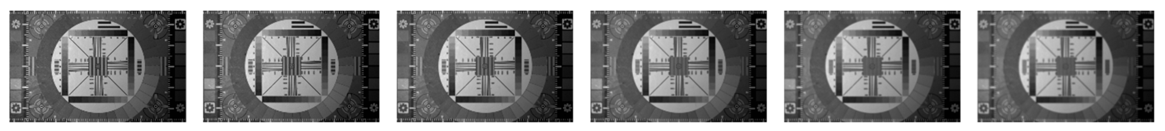
SEQ1 (cf. Figure 2) was initially used to validate our approach. To produce the six images of SEQ1, a 2D object was selected, which permitted it to be placed first in the camera’s focal plane (image Chart 1) and then in planes further and further away from the focal one (images Chart 2 to Chart 6). Blur occurs due to defocusing.
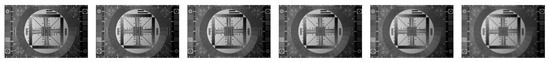
Figure 2.
SEQ 1: Chart images, Chart 1, …, Chart 6. On the left, the chart is located in the focal plane. From left to right: images progressively defocused.
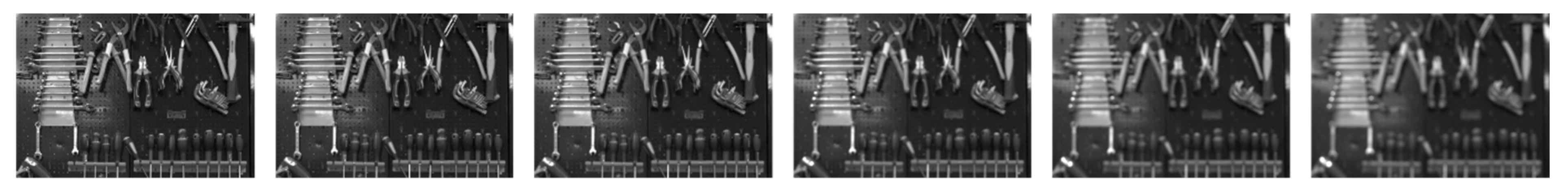
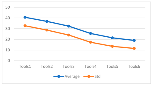
SEQ2 (cf. Figure 3) concerns images of a 3D object “Tools”. In the initial scene, tools are hanging from the same vertical board. Therefore, the main source of blur is still defocusing.
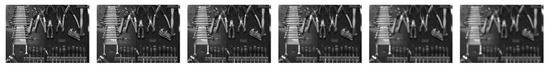
Figure 3.
SEQ 2: Tools images, Tools 1, …, Tools 6. On the left, the tools are located in the focal plane. From left to right: images progressively defocused.
2.3. Method
As proposed in [11], we choose to associate contrast maps with the studied sequence of images, but the contrast concepts we use are defined in the LIP framework to be consistent with human vision, instead of “computing the root mean square values in local pixel neighborhood”.
Based on the LIP addition , it is possible to define the additive contrast associated with a pair of pixels inside a grey level image according to:
This means that represents the grey level we must add, in the LIP sense, to the brightest grey level to reach the grey level of the darkest one. Using Formula (5), we obtain:
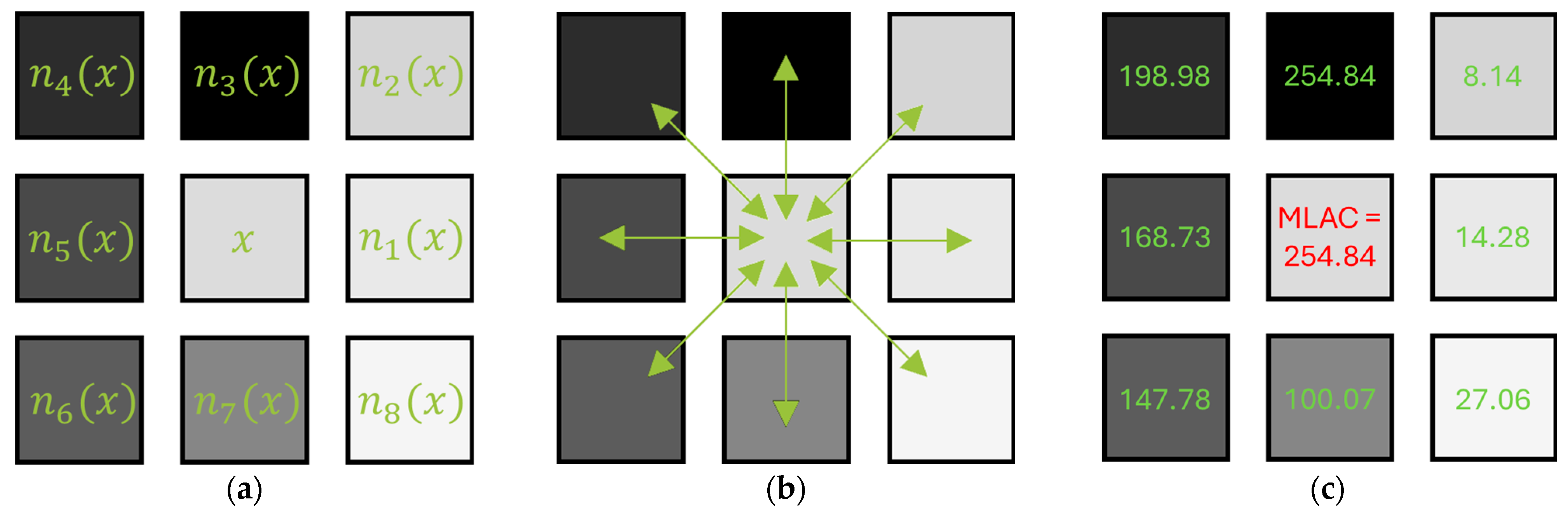
Considering a pixel it is then possible to calculate the contrast of with each of its eight neighbors for , deducing therefrom two contrast concepts:
- -
- The Average Logarithmic Additive Contrast :
- -
- The Maximal Logarithmic Additive Contrast :
To highlight the variation of f around a pixel x lying in a transition area, we prefer applying MLAC because it detects which of the eight possible directions of the square grid provides maximum contrast, corresponding to the maximal slope of f among the eight possible directions.
Figure 4 illustrates how Formula (8) is easy to calculate and can, therefore, be used by any interested reader.
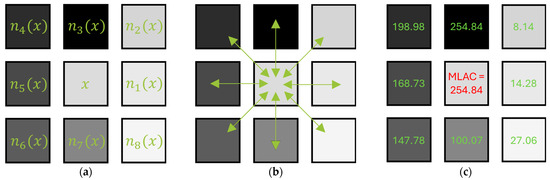
Figure 4.
Calculation of 4-(a)-Pixel and its eight neighbors 4-(b)-Calculation of for , 4-(c)-LAC values observed around .
Concerning the run-time of the MLAC method, tests were performed on standard hardware, without any specific optimization. We obtained:
43 ms per frame in Python for a 640 × 480 image (23 fps).
10 ms per frame in C++ for a 640 × 480 image (100 fps).
2.4. Results
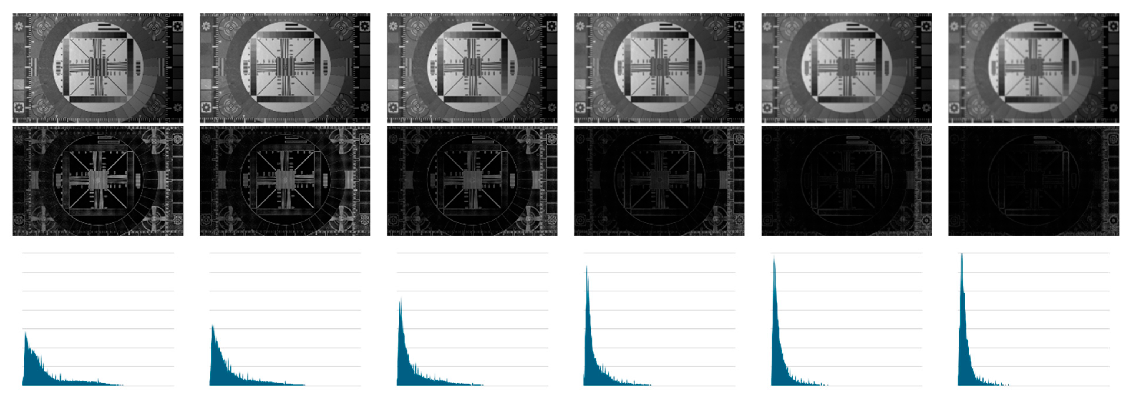
To images of SEQ1 and SEQ2, we applied the Maximal Logarithmic Additive Contrast to get the associated contrast maps. As expected, these maps present transition areas (boundaries) whose width increases with defocusing while their intensity decreases. Such observations are confirmed by the evolution of the associated greyscale histograms, whose shape moves toward the black value 0 of the greyscale as defocusing increases.
In Figure 5, we display the images of SEQ1, the associated contrast maps, and the corresponding histograms.

Figure 5.
First line: Images of SEQ1. Second line: MLAC maps. Third line: histograms associated with MLAC maps.
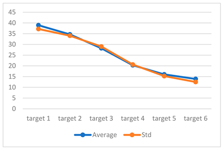
To associate measures with such observations, we calculate the average and standard deviation of previous histograms (Table 1).

Table 1.
Average and Standard Deviation of MLAC maps (SEQ1).
We observe that average and standard deviation are strongly correlated and that just one of these two basic parameters is enough to reorder the six images from SEQ1
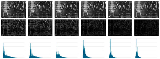
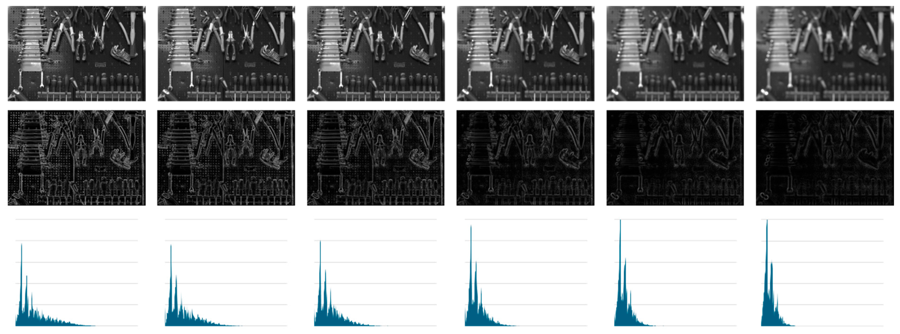
Figure 6.
First line: Images of SEQ2. Second line: MLAC maps. Line 3: histograms associated with MLAC maps.
Table 2.
Average and Standard Deviation of MLAC maps (SEQ2).
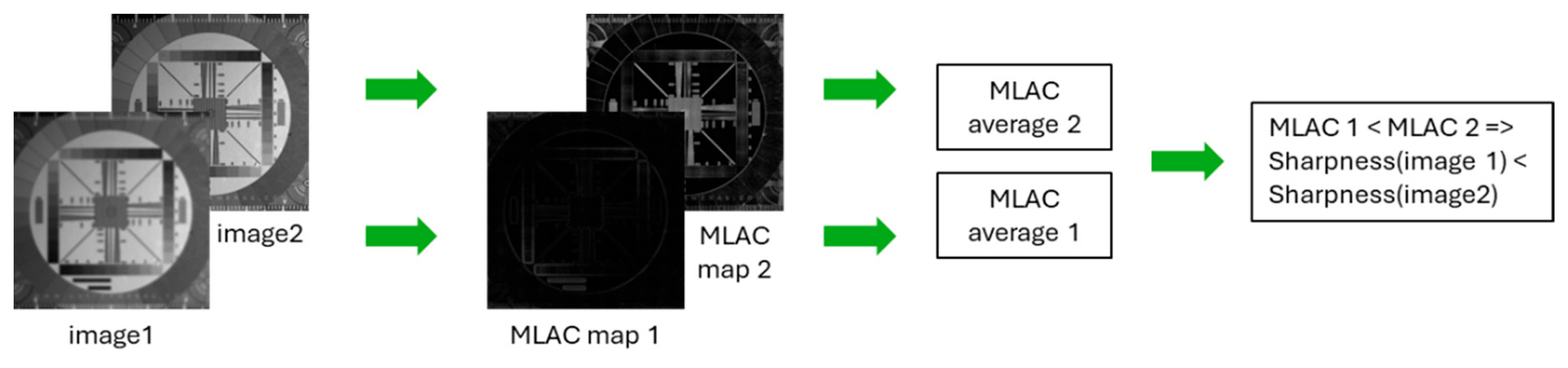
To summarize the processing pipeline of our sharpness evaluation method, we refer to following Figure 7.
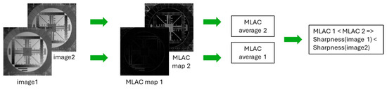
Figure 7.
Main steps of the proposed approach.
Let us note that the presented methods can be applied to a color image after the calculation of its brightness-associated image. This remark will be used in Section 3 below.
2.5. Comparison with Existing Methods
Most sharpness evaluation methods calculate parameters based on gradients or Laplacians whose values have extremely variable dynamic ranges, making them difficult to compare. Moreover, we know from experience that most of these parameters are affected by brightness variations, unlike logarithmic contrast.
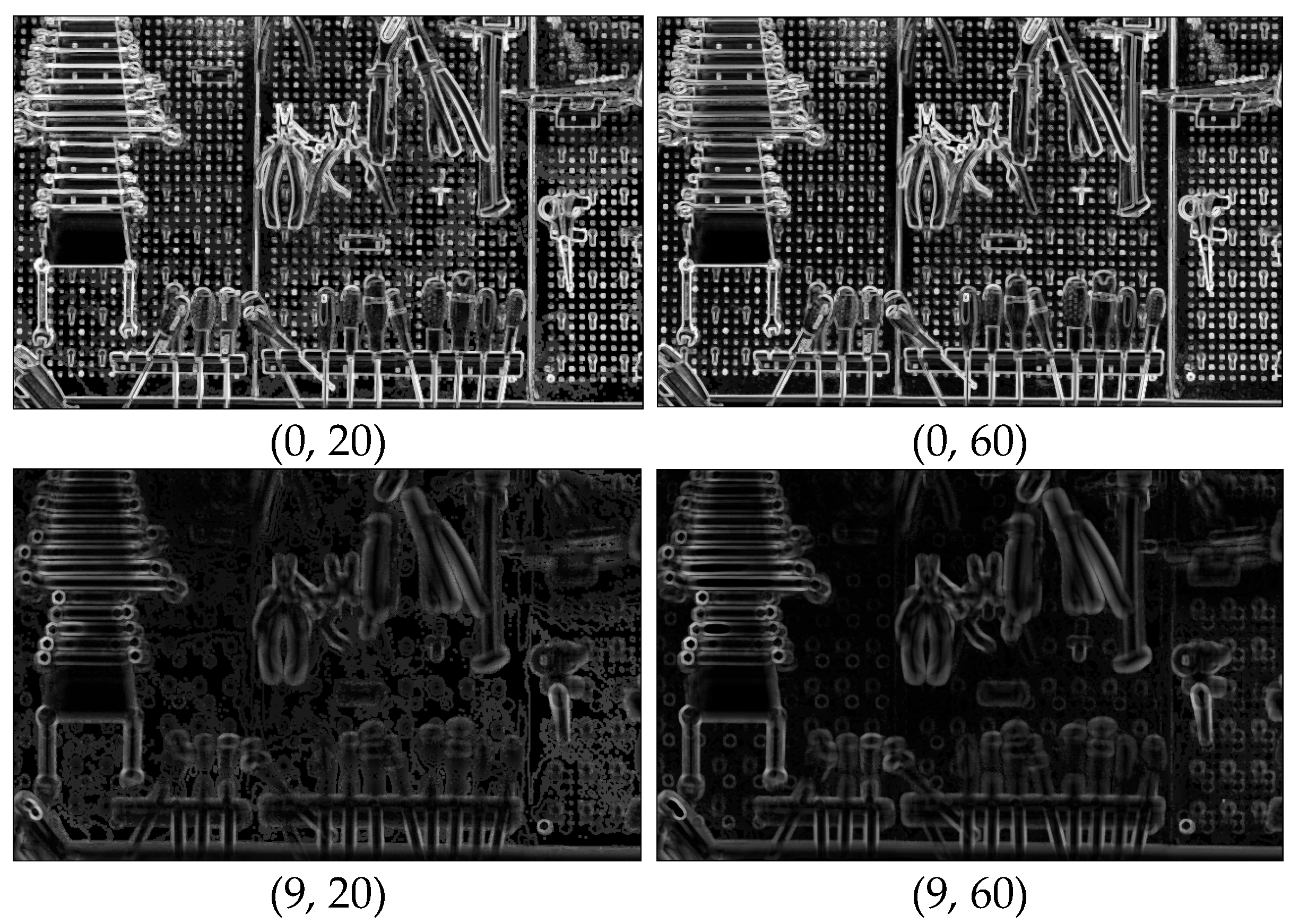
We, therefore, decided to create a third image database, SEQ3, using the SEQ2 scene with ten defocus steps numbered from 0 (focal plane) to 9 (maximum defocus) and 5 different exposure times, from 20 ms to 60 ms. Considering that the SEQ3 database contains 50 images, we have chosen to display only the 4 most representative cases in Figure 8:
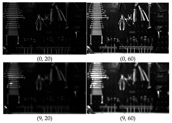
Figure 8.
Images belonging to SEQ3 are the most representative examples. (0, 20): The sharpest image acquired at 20 ms; (0, 60): The sharpest image acquired at 60 ms; (9, 20): The most defocused one acquired at 20 ms; (9, 60): The most defocused one acquired at 60 ms.
The MLAC maps were computed for the 50 images of SEQ3. In Figure 9, we display the MLAC maps corresponding to the 4 images of Figure 8.
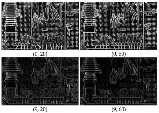
Figure 9.
Images of Figure 8: MLAC maps.
Please note that images of SEQ3 and their MLAC Maps are accessible at https://github.com/arnaud-nt2i/SharpnessEvaluationDataset/tree/main (accessed on 19 May 2025).
To compare them with the MLAC, we selected five classic methods for assessing sharpness: Local variation, Tenengrad, Brenner, Sobel variation, and Laplacian variation. These various algorithms are described in detail in the well-known paper authored by Pertuz et al. [15], and the corresponding computer codes are available at Autofocus using OpenCV: A Comparative Study of Focus Measures.
The first thing we noticed when applying these algorithms to SEQ3 is that their dynamic ranges are extremely different, making comparisons difficult to perform. Table 3 displays the values associated with each of the six methods applied to Image 0. We note that:
Table 3.
Image 0. Associated sharpness values.
- -
- For all six algorithms, values range from 33.24 to 2593.19.
- -
- The MLAC method is the only one whose values vary little as a function of exposure time.
For this reason, we decided to rescale each dynamic range from 0 to 100. The upper values correspond to the best sharpness. Results are displayed in Table 4.
Table 4.
Normalized values of SEQ3 images according to variable focus and exposure time.
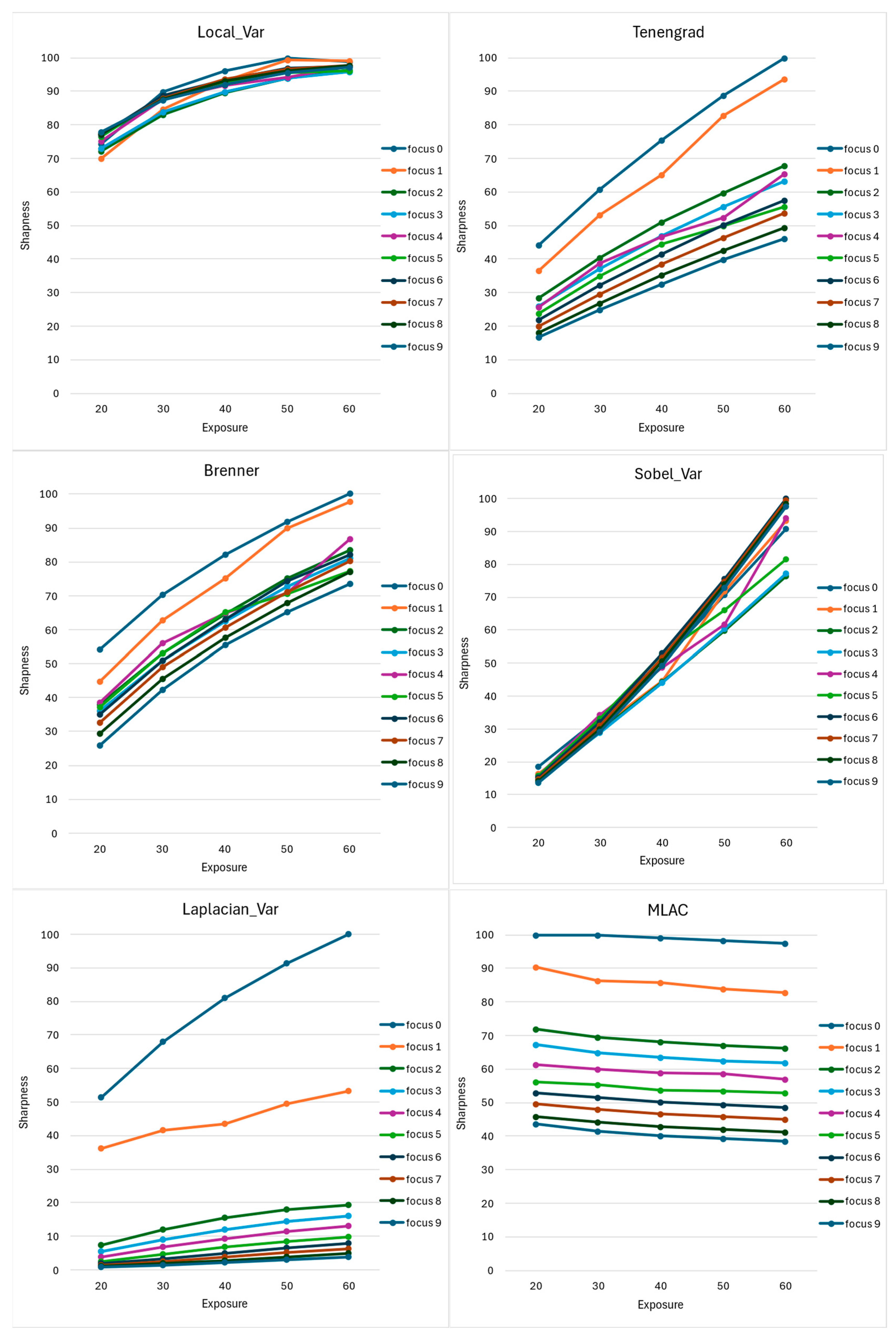
Even with normalized values associated with the 50 SEQ3 images, Table 4 is not easy to interpret. We propose to associate with each method a set of curves showing both its ability to reclassify focusing steps and its sensitivity to illumination variations (Figure 10).
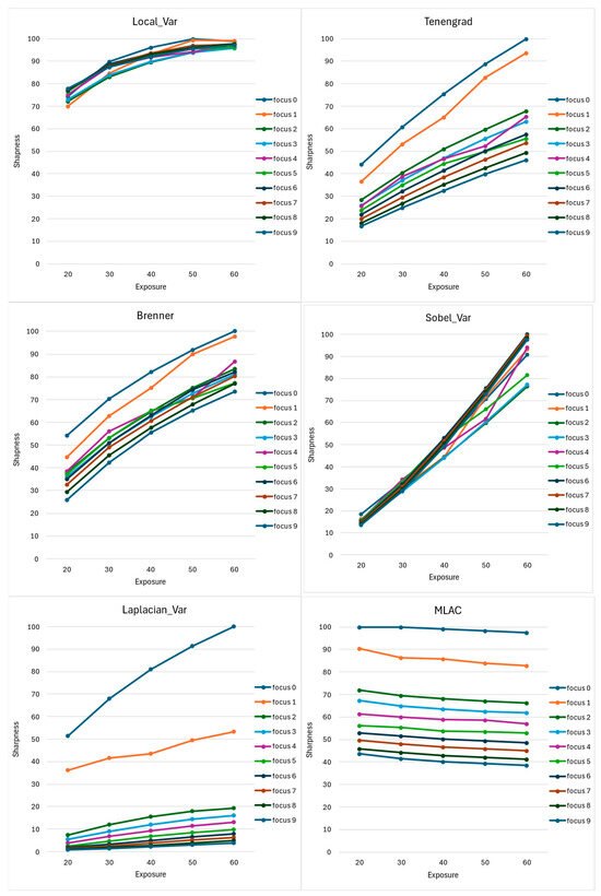
Figure 10.
For each of the six studied methods, curves are associated with each of the nine focus steps. They represent the sharpness value (vertical axis) according to the exposure time (horizontal axis).
Remarks:
- -
- The first quality we expect from a sharpness evaluation method is its ability to re-order the nine focus levels in the right order for the same exposure time. On the previous curves, this means that the curves never intersect. This property is obviously unsatisfied with the first four methods, for which we observe curve crossings. We now need to compare the Laplacian and MLAC algorithms.
- -
- The curves for the blurriest images (numbers 5, 6, 7, and 8) are less well separated for Laplacian than for MLAC.
As we claimed earlier, logarithmic contrast is theoretically insensitive to exposure time, unlike algorithms using a gradient approach. Note that insensitivity to exposure time is easily observable: the associated curve should appear horizontal for each focus level. This is not the case for Laplacian, which is therefore extremely sensitive to brightness, particularly for the sharpest images: the highest curves show the steepest slope. On the other hand, the MLAC offers almost horizontal curves.
In conclusion, the MLAC approach outperforms standard sharpness assessment methods for its ability to reclassify a sequence of progressively defocused images and its insensitivity to exposure time variations.
2.6. Possible Extensions
Based on very simple parameters, we have established the effectiveness of the notion of logarithmic contrast in reordering a sequence of images acquired with increasing defocus. Such a situation addresses the comparison between images. In the future, we plan to extend our work in at least four ways:
- -
- Define a sharpness criterion without reference.
Our first aim will be to adapt the method to obtain an absolute sharpness criterion. The results of Figure 9 concerning MLAC encourage us in this direction. They show that the MLAC value is stable for different exposure times, depends only on the quality of the focus, and increases with it.
- -
- Test other parameters than the mean and standard deviation.
Let us point out that many other metrics or parameters could be used to exploit our image sequences, for example, to compare two contrast maps or their histograms: Kullback–Leibler divergence entropy [16,17], Hellinger distance (cf. application example [18]), and Wasserstein distance [19]. Readers interested in these techniques will find additional material in Appendix A.
- -
- Introduce local processing.
As it currently stands, the MLAC method appears very effective for comparing the sharpness of two images. For images containing regions with different degrees of blur, local processing would then be necessary.
Moreover, after a calibration phase, such local processing could be used to roughly assess the distance of objects in the scene from the sensor.
It can also be used to compare two blur removal methods applied to the same image. This will be particularly interesting for thermal images, which are naturally blurred.
- -
- Undertake subjective user validation.
For the interested reader, MLAC’s insensitivity to brightness is a direct consequence of [20] in which variations in exposure time are modelled by the logarithmic addition or the subtraction of a constant, and it is obvious that such an addition/subtraction does not modify the logarithmic additive contrast. The method can, therefore, be applied to very low-light images that have been enhanced by logarithmic subtraction of a constant.
In the following Section 3, we present two applications of the MLAC method:
- -
- Comparison of two Super-Resolution algorithms.
- -
- Control of an autofocus during the automatic screening of a cell preparation using a microscope.
3. Applications
3.1. Comparison of Two Super-Resolution Algorithms
In image processing, there is often a need to improve spatial resolution to get a better level of detail. This is classically achieved by means of Super Resolution algorithms (SR algorithms). Numerous methods exist, including classic approaches [21] such as bilinear interpolation, which takes only 4 pixels into account, or Bicubic Interpolation (BI), which considers a neighborhood of 16 pixels. Recently, Zhang et al. [22] proposed a deep super-resolver called BSRGAN using a complex image degradation model consisting of downsampling, random blur, and various noise degradations.
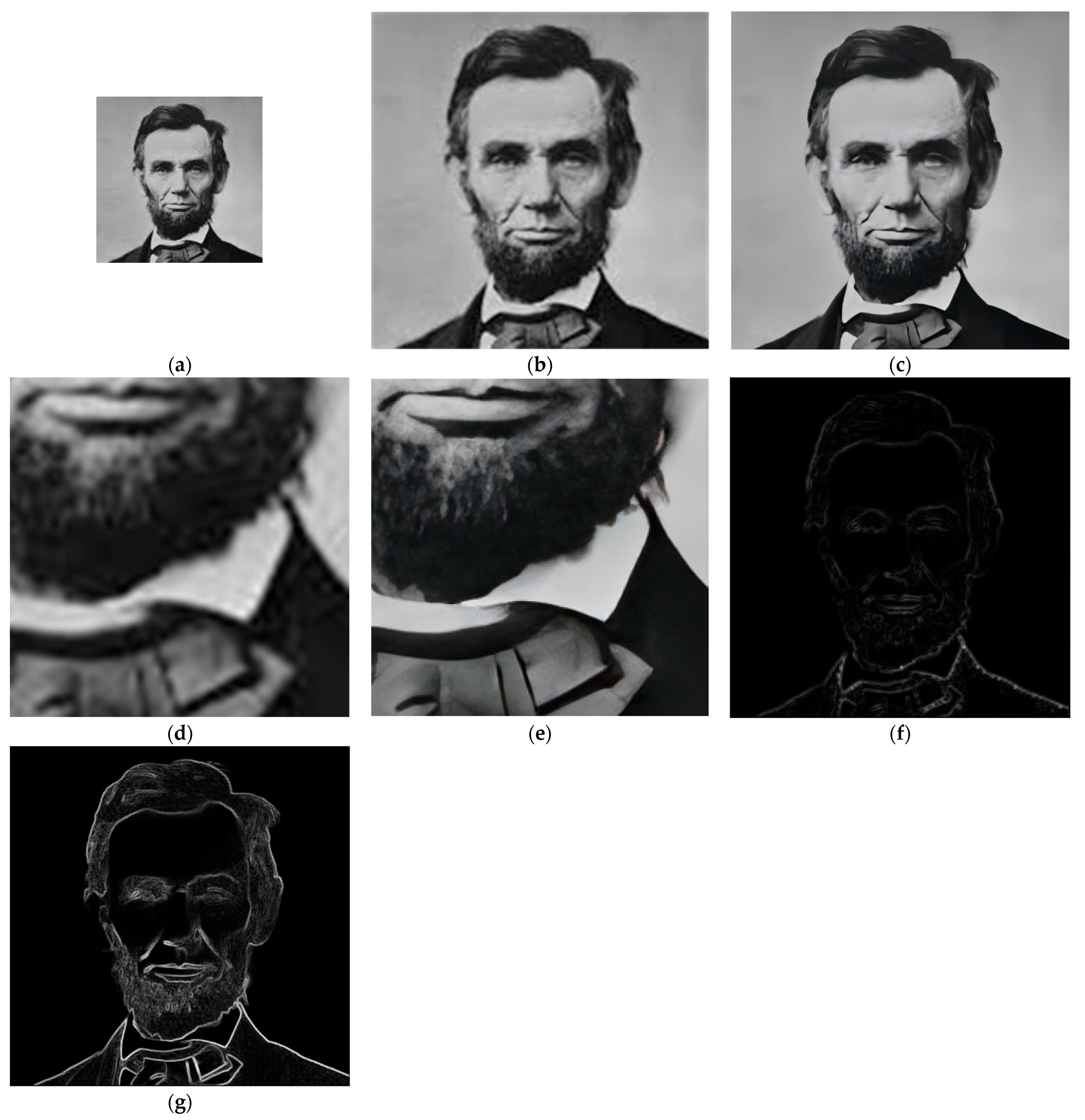
In the following Figure 11, we associate two SRx2 images with the initial image Lincoln using the BI and BSRGAN algorithms, respectively, and we apply them to the Maximal Logarithmic Additive Contrast MLAC.
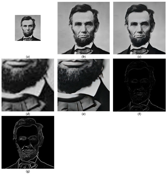
Figure 11.
Comparison of two SR algorithms. (a) Initial image “Lincoln”, (b) Lincoln BIx2, (c) Lincoln BSRGANx2, (d) Details on (b), (e) Details on (c), (f) MLAC applied to (b), (g) MLAC applied to (c).
In the detailed images, we can clearly observe that the shirt collar, the bow tie, and the beard hairs are much sharper on Figure 11e than on Figure 11d. The boundaries (images Figure 11f,g) are clearly thicker and less contrasted with the bicubic interpolation algorithm, but this comparison is not really fair, given that BSRGAN includes image enhancements, particularly regarding blur. We will, therefore, add to the BIx2 algorithm a blur removal step based on the well-known Unsharp Masking (UM) technique, producing the algorithm denoted UM(BIx2).
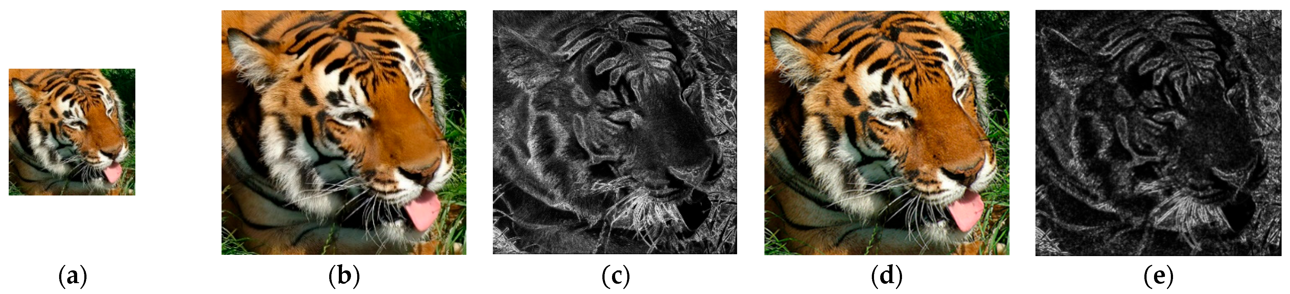
Displayed in the following Figure 12, we consider the initial color image, “Tiger”, to which we associate its grey-level luminance image, then proceed as for the Lincoln image.
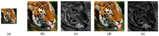
Figure 12.
Comparison of BSRGANx2 and UM(BIx2) methods by means of the associated MLAC maps (a) Initial image “Tiger”, (b) BSRGANx2, (c) MLAC (b), (d) UM(BIx2) (b), (e) MLAC (d).
As in Figure 11, we can see that the black stripes on the tiger’s head are more accurately detected by BSRGANx2 than UM(Bix2).
The results presented in Table 5 confirm the superiority of BSRGANx2 compared to UM(BIx2).
Table 5.
Comparison between BSRGANx2 and UM(BIx2).
3.2. Automated Autofocus Control
This section concerns images of cells acquired by microscopy during the screening of a vaginal smear with the aim of detecting cervical cancer.
The cell preparation is presented on a slide moved by a programmable stage. All along the stage motion, it is necessary to perform autofocusing because hundreds of microscope fields have to be explored, and the slide is not perfectly flat.
To simulate this situation, we chose a cell field that we placed in the focal plane of the camera, producing the sharpest possible image “0”.
We, then, proceeded to progressive defocusing with a constant step, thus obtaining 9 images on either side of the “0” location, numbered from −9 to −1 for those closer to the camera and from 1 to 9 for those further than the focal plane. In Figure 13 considering that it is not appropriate to show all nineteen images, we decided to display only the sharpest images: “−1”, “0”, “1”, and the blurriest ones: “−9”, “−8”, “8”, and “9”.
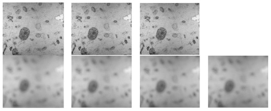
Figure 13.
First line: Images “−1”, “0”, and “1”. Second line: Images “−9”, “−8”, “8”, and “9”.
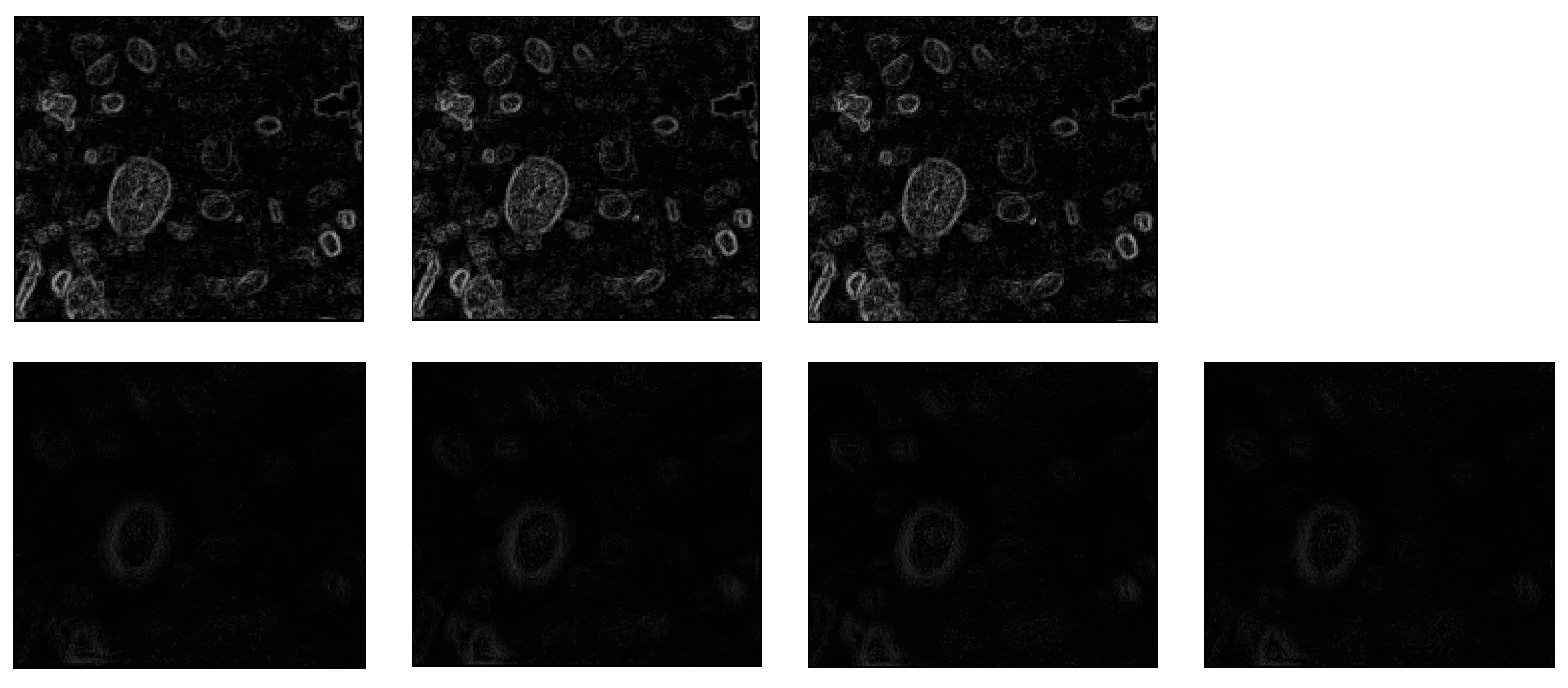
For each of the 19 images, the MLAC map was calculated. The maps associated with images of Figure 13 are presented in Figure 14. Due to their low-light level, their brightness has been slightly increased to make them visually interpretable.

Figure 14.
First line: MLAC maps of Images “−1”, “0”, and “1”. Second line: MLAC maps of Images “−9”, “−8”, “8”, and “9”.
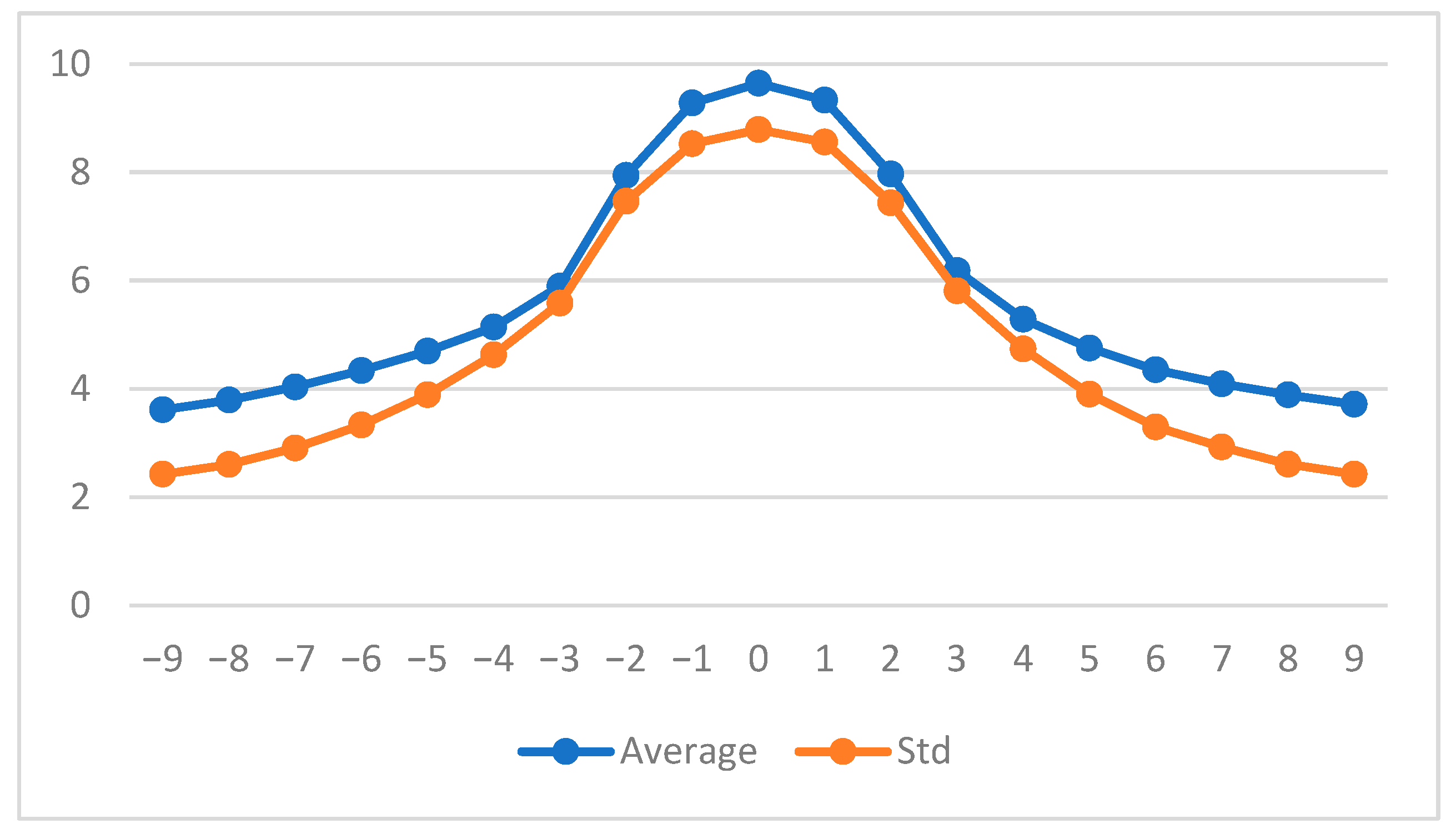
As expected, the boundaries appear thicker and less contrasted on defocused images, resulting in lower values for the associated mean and standard deviation (see Figure 15).

Figure 15.
Grey level average (in blue) and standard deviation (in red) calculated on the 19 MLAC maps.
Each of the parameters “Average” or “Standard deviation” permits to precisely select the sharpest image and is then able to perform autofocusing.
4. General Conclusions
In this paper, we set ourselves the main objective of finding a convincing alternative to the use of gradients for assessing image blur. This was achieved by choosing the LIP framework, due to its strong mathematical and optical properties combined with its consistency with human vision. It has been shown that the notion of Maximal Logarithmic Additive Contrast (MLAC) is perfectly suited to the evaluation of blur and can be exploited with very simple parameters such as the mean or standard deviation. The corresponding algorithm is executable in real-time (100 fps for 640 × 480 images).
Compared to five standard methods, MLAC has proved to be the best performer for evaluating sharpness and was the only one to show insensitivity to variations in exposure time.
We suggested several potential applications for the proposed approach, like comparing two Super Resolution methods or driving a self-focusing action. However, the study initiated here opens a wide range of perspectives, some of which are outlined in Appendix A. Our ambition is now to carry out similar work on other image quality criteria, such as contrast assessment. As this latter notion is very closely linked to human vision, it seems appropriate to us to retain the LIP context. After studying the boundaries, considered as transition zones, we plan to study more precisely the relatively homogeneous areas delimited by these boundaries and to associate them with an average logarithmic internal contrast [13], somewhat comparable to entropy. In parallel, the contrast between adjacent homogeneous regions will be estimated, and both information should be combined to propose the notion of global perceived contrast.
Author Contributions
Conceptualization, A.P., M.C. and M.J.; methodology, M.J., D.G. and F.M.; software, A.P. and M.C.; formal analysis A.P. and M.J.; resources, A.P.; data curation, A.P. and M.C.; writing—original draft preparation, A.P.; writing—review and editing, M.J. and A.P.; supervision, D.G. and F.M.; project administration, M.J. All authors have read and agreed to the published version of the manuscript.
Funding
This research received no external funding.
Data Availability Statement
The dataset used in this study, comprising all images presented in the manuscript, is freely available at https://github.com/arnaud-nt2i/SharpnessEvaluationDataset, accessed on 19 May 2025.
Conflicts of Interest
Authors Arnaud Pauwelyn and Maxime Carré were employed by NT2I Company. The remaining authors declare that the research was conducted in the absence of any commercial or financial relationships that could be construed as a potential conflict of interest.
Appendix A
In the present paper, we deliberately limited our presentation to very simple parameters calculated from MLAC maps, such as average or standard deviation. We plan to extract other parameters based on distances in the mathematical sense, either between the MLAC maps themselves or between their histograms.
- Kullback–Leibler divergence
The Kullback–Leibler divergence (or K–L divergence or relative entropy) is a measure of dissimilarity between two probability distributions. The respective histograms and of two images and are considered as two discrete probability distributions defined on the numerical grey scale The Kullback–Leibler divergence of with respect to is then expressed as follows:
- b.
- Hellinger metric
The Hellinger distance is defined according to:
It is easy to check that satisfies the mathematical properties required to be a metric, which include the triangular inequality.
- c.
- Wasserstein distance
The Wasserstein distance between histograms and is calculated as follows:
where represents the mathematical expectation.
References
- Zhu, M.; Yu, L.; Wang, Z.; Ke, Z.; Zhi, C. A Survey on Objective Evaluation of Image Sharpness. Appl. Sci. 2023, 13, 2652. [Google Scholar] [CrossRef]
- Elder, J.H.; Zucker, S.W. Local scale control for edge detection and blur estimation. IEEE Trans. Pattern Anal. Mach. Intell. 1998, 20, 699–716. [Google Scholar] [CrossRef]
- Kim, D.-O.; Han, H.-S.; Park, R.-H. Gradient information-based image quality metric. IEEE Trans. Consum. Electron. 2010, 56, 930–936. [Google Scholar] [CrossRef]
- Xue, W.; Zhang, L.; Mou, X.; Bovik, A.C. Gradient magnitude similarity deviation: A highly efficient perceptual image quality index. IEEE Trans. Image Process. 2013, 23, 684–695. [Google Scholar] [CrossRef] [PubMed]
- Liu, Z.; Hong, H.; Gan, Z.; Wang, J.; Chen, Y. An improved method for evaluating image sharpness based on edge information. Appl. Sci. 2022, 12, 6712. [Google Scholar] [CrossRef]
- Cong, H.; Fu, L.; Zhang, R.; Zhang, Y.; Wang, H.; He, J.; Gao, J. Image Quality Assessment with Gradient Siamese Network. In Proceedings of the IEEE/CVF Conference on Computer Vision and Pattern Recognition (CVPR), Seattle, WA, USA, 17–21 June 2022; pp. 1201–1210. [Google Scholar]
- Chen, L.; Pan, J.; Yang, J.; Wang, M. CS-Net: Deep Multi-Branch Network Considering Scene Features for Sharpness Assessment of Remote Sensing Images. IEEE Trans. Geosci. Remote Sens. 2024, 62, 5404314. [Google Scholar] [CrossRef]
- Yang, M.; Yin, G.; Wang, H.; Dong, J.; Xie, Z.; Zheng, B. A underwater sequence image dataset for sharpness and color analysis. Sensors 2022, 22, 3550. [Google Scholar] [CrossRef] [PubMed]
- Ryu, J.K.; Kim, K.H.; Otgonbaatar, C.; Kim, D.S.; Shim, H.; Seo, J.W. Improved stent sharpness evaluation with super-resolution deep learning reconstruction in coronary CT angiography. Br. J. Radiol. 2024, 97, 1286–1294. [Google Scholar] [CrossRef] [PubMed]
- Wan, J.; Zhang, X.; Yang, W.; Zhang, C.; Lei, M.; Dong, Z. A calibration method for defocused cameras based on defocus blur estimation. Measurement 2024, 235, 115045. [Google Scholar] [CrossRef]
- Gvozden, G.; Grgic, S.; Grgic, M. Blind image sharpness assessment based on local contrast map statistics. J. Vis. Commun. Image Represent. 2018, 50, 145–158. [Google Scholar] [CrossRef]
- Jourlin, M.; Pinoli, J.-C. A model for Logarithmic Image Processing. J. Microsc. 1988, 149, 21–35. [Google Scholar] [CrossRef]
- Jourlin, M. Logarithmic Image Processing: Theory and Applications; Academic Press: Cambridge, MA, USA, 2016; Volume 195, 260p. [Google Scholar]
- Brailean, J.; Sullivan, B.; Chen, C.; Giger, M. Evaluating the em algorithm using a human visual fidelity criterion. Int. Conf. Acoust. Speech Signal Process. 1991, 6, 2957–2960. [Google Scholar]
- Pertuz, S.; Puig, D.; Garcia, M.A. Analysis of focus measure operators for shape-from-focus. Pattern Recognit. 2013, 46, 1415–1432. [Google Scholar] [CrossRef]
- Kullback, S.; Leibler, R.A. On information and sufficiency. Ann. Math. Stat. 1951, 22, 79–86. [Google Scholar] [CrossRef]
- Pheng, H.S.; Shamsuddin, S.M.; Leng, W.Y.; Alwee, R. Kullback-Leibler divergence for image quantitative evaluation. AIP Conf. Proc. 2016, 1750, 020003. [Google Scholar]
- Gupta, A.; Kochchar, S.K.; Joshi, A. Image Classifier based on Histogram Matching and Outlier Detection using Hellinger distance. J. Appl. Data Sci. 2023, 4, 407–413. [Google Scholar] [CrossRef]
- Dobrushin, R.L. Prescribing a system of random variables by conditional distributions. Theory Probab. Its Appl. 1970, 15, 458–486. [Google Scholar] [CrossRef]
- Carré, M.; Jourlin, M. Brightness Spatial Stabilization in the LIP framework. In Proceedings of the 14th International Congress for Stereology and Image Analysis, Liège, Belgium, 7–10 July 2015. [Google Scholar]
- Parsania, P.S.; Virparia, P.V. A Review: Image Interpolation Techniques for Image Scaling. Int. J. Innov. Res. Comput. Commun. Eng. 2014, 2, 7409–7414. [Google Scholar] [CrossRef]
- Zhang, K.; Liang, J.; Van Gool, L.; Timofte, R. Designing a Practical Degradation Model for Deep Blind Image Super-Resolution. In Proceedings of the IEEE/CVF International Conference on Computer Vision (ICCV), Montreal, QC, Canada, 10–17 October 2021; pp. 4791–4800. [Google Scholar]


Disclaimer/Publisher’s Note: The statements, opinions and data contained in all publications are solely those of the individual author(s) and contributor(s) and not of MDPI and/or the editor(s). MDPI and/or the editor(s) disclaim responsibility for any injury to people or property resulting from any ideas, methods, instructions or products referred to in the content. |
© 2025 by the authors. Licensee MDPI, Basel, Switzerland. This article is an open access article distributed under the terms and conditions of the Creative Commons Attribution (CC BY) license (https://creativecommons.org/licenses/by/4.0/).