Machine Learning-Based Analysis of Travel Mode Preferences: Neural and Boosting Model Comparison Using Stated Preference Data from Thailand’s Emerging High-Speed Rail Network

Abstract

This study examines travel mode choice behavior within the context of Thailand’s emerging high-speed rail (HSR) development. It conducts a comparative assessment of predictive capabilities between the conventional Multinomial Logit (MNL) framework and advanced data-driven methodologies, including gradient boosting algorithms (Extreme Gradient Boosting, Light Gradient Boosting Machine, Categorical Boosting) and neural network architectures (Deep Neural Network, Convolutional Neural Network). The analysis leverages stated preference (SP) data and employs Bayesian optimization in conjunction with a stratified 10-fold cross-validation scheme to ensure model robustness. CatBoost emerges as the top-performing model (area under the curve = 0.9113; accuracy = 0.7557), highlighting travel cost, service frequency, and waiting time as the most influential determinants. These findings underscore the effectiveness of machine learning approaches in capturing complex behavioral patterns, providing empirical evidence to guide high-speed rail policy development in low- and middle-income countries. Practical implications include optimizing fare structures, enhancing service quality, and improving station accessibility to support sustainable adoption.

1. Introduction

In recent decades, Thailand has experienced rapid urbanization, resulting in a substantial increase in travel demand. This surge has led to congestion in public transportation systems and a growing reliance on private vehicles. High-speed rail (HSR) has emerged as a key solution to address these issues, offering the potential to significantly reduce travel times, enhance intercity connectivity, and promote economic development across various regions [1,2,3]. In Thailand, collaboration with China on the development of HSR is expected to substantially reshape the nation’s transportation landscape by providing an alternative to private cars, intercity buses, and air travel [4].

The development of HSR also aligns with Thailand’s commitments under the Sustainable Development Goals (SDGs), particularly SDG 9, which focuses on building resilient infrastructure; SDG 11, aimed at making cities inclusive, safe, resilient, and sustainable; and SDG 13, which calls for urgent action to combat climate change and its impacts. HSR development is not only anticipated to reduce reliance on fossil fuels but also to foster sustainable urban connectivity and mitigate carbon emissions from long-distance transportation [5]. Furthermore, the Thai government has incorporated HSR into its National Action Plan for advancing the SDGs, positioning the rail network as a crucial strategy for reducing infrastructure disparities and promoting inclusive growth nationwide.

From an infrastructure perspective, Thailand is currently undertaking the construction of four major HSR lines—the northern, eastern, northeastern, and southern corridors—designed to enhance economic development, trade, tourism, and regional connectivity. A particularly significant project is the Thai–Lao–Chinese HSR, a collaboration between the Thai and Chinese governments. This line will connect Bangkok’s Bang Sue Grand Station with Laos and onward to China, spanning approximately 377 miles across eight provinces through eleven stations. The project is divided into two phases: the Bangkok–Nakhon Ratchasima section (155 miles), currently under construction, and the Nakhon Ratchasima–Nong Khai section (222 miles), which will link to China’s HSR network via Laos. Full completion is expected by 2030 [6,7]. This project is anticipated to significantly influence intercity travel behavior and attract users away from private vehicles and low-cost airlines.

Nevertheless, predicting travel mode choice in response to HSR introduction remains challenging due to the complex interplay of factors such as travel time, cost, station accessibility, waiting time, and service frequency [8,9,10,11,12,13]. Traditionally, travel mode choice modeling has been grounded in the Random Utility Maximization (RUM) framework, with the Multinomial Logit (MNL) model serving as the dominant tool due to its theoretical rigor, ease of interpretation, and suitability for analyzing both individual-specific and alternative-specific variables [14,15,16,17]. However, MNL models suffer from several limitations, including the Independence of Irrelevant Alternatives (IIA) assumption, limited capacity to capture nonlinear relationships, and reduced predictive performance when dealing with high-dimensional or correlated datasets.

To overcome these limitations, extensions such as the Nested Logit (NL), Cross-Nested Logit (CNL), and Mixed Logit (ML) models have been developed, offering improved behavioral flexibility [18,19,20,21,22]. Nevertheless, these models still require predefined functional forms and often involve considerable computational complexity. Recent advancements in machine learning (ML) and deep learning (DL) offer promising alternatives, capable of capturing complex, nonlinear relationships without assuming specific functional forms. Ensemble tree methods, such as Random Forest, Extreme Gradient Boosting (XGBoost), Light Gradient Boosting Machine (LightGBM), and Categorical Boosting(CatBoost), have proven to deliver superior predictive performance in travel mode choice applications [23,24,25,26,27], while Deep Neural Networks (DNNs) and Convolutional Neural Networks (CNNs) have shown remarkable capabilities in processing structured and high-dimensional data [28,29,30,31].

Although machine learning (ML) and deep learning (DL) models are widely acknowledged for their superior predictive capabilities, concerns have been persistently raised regarding their limited interpretability and opacity, commonly referred to as the “black-box” phenomenon [31,32]. To address this challenge and enhance model explain ability, the present study employs Shapley Additive Explanations (SHAP), a solution grounded in cooperative game theory, to elucidate the internal logic of the models and identify the most influential predictors associated with travel mode decisions [33]. While the use of ML techniques in travel behavior analysis has expanded, rigorous comparative studies between ML/DL frameworks and conventional econometric models, particularly those utilizing stated preference (SP) data in the context of high-speed rail (HSR) development in Thailand, remain limited. This research endeavors to bridge this empirical gap by conducting a systematic evaluation of the predictive performance of MNL, XGBoost, LightGBM, CatBoost, DNN, and CNN models using large-scale SP data collected from 3200 respondents across 16 provinces. A standardized data preprocessing framework, Bayesian hyperparameter optimization, and 10-fold cross-validation are employed to ensure rigorous model evaluation. Furthermore, SHAP analysis is utilized to enhance transparency and provide insights into the key factors driving travel mode choices. This research offers one of the first comprehensive evaluations integrating traditional econometric models and advanced ML/DL techniques in the emerging context of HSR in a developing country, contributing valuable insights for future transportation planning and sustainable mobility policymaking.

2. Methodology and Data Analysis

The research methodology, as depicted in Figure 1, follows a systematic and structured approach, commencing with stated preference surveys and data validation to ensure data accuracy and reliability. Subsequently, the dataset is partitioned into training (X_train, y_train) and testing (X_test, y_test) sets to facilitate model development. The study employs multiple analytical frameworks, including deep learning comprising Convolutional Neural Networks (CNNs) and Deep Neural Networks (DNNs) as well as Multinomial Logit (MNL) and Gradient Boosting methods, such as XGBoost, LightGBM, and CatBoost. To enhance model performance, hyperparameter tuning is conducted, followed by a comparative evaluation utilizing cross-validation techniques and performance metrics. In the final stage, a judgment assessment is performed to determine the acceptability of the model results. Upon validation, the most optimized model undergoes further interpretability analysis using Shapley Additive Explanations (SHAP) to identify the key determinants influencing travel mode choice. The dataset was handled and examined utilizing Python 3.11 through Anaconda, with the final preparation phase taking approximately two hours. A 13th-generation Intel Core i9-13900H processor running at 2.60 GHz, combined with 32 GB of RAM, powered the system used for computational analysis, supporting high efficiency and processing speed.

2.1. Survey Design

This study examines future travel mode preferences, encompassing buses, traditional rail, air transport, and high-speed rail (HSR), through advanced machine learning techniques. Data were obtained from a nationwide survey encompassing four major geographic zones of Thailand: The north, northeast, central, and south. The analysis aims to uncover the key determinants influencing travel behavior and choice decisions [29].

Target provinces were selected based on their strategic potential for future HSR development, with selection criteria including economic vitality and infrastructural significance as of 2022 [34]. Incorporating provinces with varying socioeconomic and infrastructural profiles across the regions supports the national representativeness of the findings [35].

The survey involved in-person interviews with adults aged 18 and above, covering 16 provinces and yielding 3200 valid responses, equally distributed across provinces (n = 200 each). A non-probability sampling strategy was employed to ensure regional coverage, mitigate selection bias, and enhance result robustness. The sample size adheres to machine learning best practices, falling within the suggested range of 50 to 1000 observations per target class, four in this case [36].

The questionnaire comprised two components: respondents’ socioeconomic information and a stated preference (SP) experiment using a choice-based design. Participants indicated their preferred travel mode under hypothetical future HSR scenarios, considering factors such as station accessibility, waiting duration, total journey time, cost, and service frequency, providing realistic behavioral insights [37,38].

2.2. Questionnaire Design

The set of explanatory variables incorporated into the choice-based survey design reflects critical service attributes known to influence individual travel mode decisions. These include the duration required to reach the departure station, the delay experienced prior to boarding, and the in-vehicle journey duration between the origin and destination. Additionally, the survey accounts for the direct financial expenditure borne by the traveler in the form of out-of-pocket fare, as well as the interval between consecutive scheduled services. These attributes were carefully selected to capture the key trade-offs faced by travelers in real-world decision-making scenarios. Collectively, they provide a robust foundation for analyzing modal preferences and quantifying the influence of service characteristics on travel behavior. A summary of these variables and their operational definitions is presented in

Table 1. Attribute Levels for Travel Modes.

Attribute	Bus	Train	Airplane	HSR (Levels 1)	HSR (Levels 2)
Access time (Station approach duration: minute)	10	10	30	10	15
Waiting time (Pre-departure delay: minute)	15	10	120	15	10
Travel (Time In-vehicle journey duration: minute)	720	720	135	190	220
Travel cost (Out-of-pocket fare: bath)	750	300	3000	1050	1400
Frequency times (Scheduled service interval: minute)	30	150	120	190	220

. Each feature was defined across multiple value tiers to mirror plausible travel conditions, thereby enhancing the reliability of respondents’ stated selections. This stated preference task concentrated along the Bangkok–Chiang Mai axis, spanning approximately 435 miles, was recognized as a strategic route due to the competitive dynamic between high-speed rail (HSR) and traditional transport alternatives.

As HSR had not yet been implemented during the survey period, assumptions related to travel time, fare levels, service intervals, and waiting durations were based on government forecasts [39]. Additional scenario parameters were informed by previous empirical research to incorporate insights into traveler preferences, operational performance, and market dynamics. Given the reliance on forecasted data, uncertainties may arise due to unexpected disruptions, infrastructure constraints, fare policy changes, or broader system dynamics. These uncertainties may affect projected demand and policy decisions. To improve scenario realism, adjustments were applied to align assumptions with actual system parameters. Reference values for waiting times were obtained from national bus and rail booking platforms [40] and airline reservation systems [41]. For competing modes, information on travel time, pricing, and scheduling was derived from official fare tables and transit timetables [42], allowing direct comparison with HSR. Adjustments were also made to access durations to account for specific constraints—such as extended airport check-in and security procedures. The finalized dataset was validated using empirical travel history and survey-based feedback to strengthen its reliability. This study assessed five core attributes across three existing travel alternatives, along with two hypothetical HSR options using a standardized factorial design.

The experimental design produced 96 total choice sets, derived from three service types, 15 attribute combinations, and 25 replications. To reduce respondent burden, a fractional factorial design was employed, dividing the sets into eight blocks containing twelve alternatives each, with each participant assigned to a single block. This structure balanced statistical precision with manageable cognitive demand [43].

2.3. Data and Variables

To prepare the stated preference (SP) survey data for machine learning applications, a preprocessing phase was carried out involving data cleansing, the handling of missing or inconsistent entries, and the normalization of continuous variables. Categorical variables were transformed using one-hot or ordinal encoding techniques. Each of the 3200 respondents participated in twelve hypothetical choice tasks, with each task presenting four alternatives: bus, train, airplane, and high-speed rail (HSR), yielding a total of 38,400 data points. The dependent variable (Y) denoted the travel mode selected by the respondent (coded as 1 = bus, 2 = train, 3 = airplane, 4 = HSR), while the predictor variables (X) comprised both quantitative factors (e.g., fare, duration) and sociodemographic indicators (e.g., gender, income level, vehicle ownership).

The data structure was organized such that each respondent’s choice set was represented by four separate records, one for each mode, where the selected alternative was labeled as Y = 1 and non-chosen alternatives as Y = 0. For instance, if train was selected, then that record was marked Y = 1 while the others were assigned Y = 0. This encoding process produced a final dataset of 38,400 rows encompassing both trip characteristics and individual-level features. To facilitate model development and validation, the dataset was randomly partitioned into training (80%) and testing (20%) subsets.

Dataset Structuring and Preprocessing

Following the collection of stated preference (SP) survey responses, the dataset underwent a comprehensive preprocessing workflow tailored to support predictive modeling using machine learning techniques. This phase involved cleaning raw entries, restructuring categorical data, and formatting the choice set architecture. Any incomplete or inconsistent records were removed, continuous variables were normalized, and categorical features including gender, household income, and private vehicle ownership were transformed using suitable encoding strategies, such as binary (one-hot) and ordinal schemes.

Each of the 3200 participants evaluated 12 hypothetical travel scenarios, yielding a dataset comprising 38,400 observations. In each scenario, respondents were asked to choose among four transportation modes: bus, conventional rail, air travel, and high-speed rail (HSR). These options were differentiated based on key service characteristics, namely access time, wait duration, total travel time, and fare cost. The response variable (Y) indicated the selected alternative, coded as 1 for the chosen mode and 0 for the others. Each option was assigned a numeric identifier from 1 to 4. The predictor variables (X) encompassed both operational attributes and sociodemographic details.

The dataset was organized such that each row represented one travel alternative within a respondent’s choice set. After preprocessing, the dataset was divided into training (80%) and testing (20%) subsets to facilitate model validation and performance evaluation.

2.4. Multinomial Logit Model for Mode Choice Estimation

The modeling framework is grounded in the assumption that each transport alternative embedded in the experimental design delivers distinct utility to decision-makers, thereby influencing their travel behavior. The probability that an individual selects a given option increases as its associated utility becomes relatively more favorable compared to competing alternatives. The Multinomial Logit (MNL) model expresses this probability as follows:

$${\mathrm{P}}_{\left(\mathrm{i}\right)}={\displaystyle \frac{e^{\mathrm{U}\mathrm{i}}}{\sum _{j\in J}{e}^{\mathrm{U}\mathrm{j}}}}$$

(1)

where:

${\mathrm{P}}_{\left(\mathrm{i}\right)}$ represents the probability that alternative i is selected;

Ui and Uj denote the systematic utilities corresponding to alternatives i and j, respectively;

J is the total number of competing alternatives considered in the model.

2.5. Deep Neural Network (DNN)

Deep Neural Networks (DNNs) are particularly effective in handling problems characterized by high nonlinearity, especially in cases involving unstructured data such as images, videos, or continuous data streams. In such complex scenarios, incorporating multiple hidden layers into a traditional Multilayer Perceptron (MLP) significantly enhances its ability to capture intricate patterns and improve predictive performance. These architectures, commonly referred to as Deep Multilayer Perceptron (DMLPs) or Deep Neural Networks (DNNs), form the foundation of modern deep learning methodologies [44,45].

2.6. Convolutional Neural Network (CNN)

Convolutional Neural Networks (CNNs) represent one of the most widely used and effective deep learning architectures, particularly in tasks requiring the extraction of hierarchical features to classify input data. These networks are particularly well suited for applications involving image and video processing, where features need to be captured at multiple levels of abstraction. The core operation of a CNN is convolution, which is performed using filters (also referred to as kernels). In the case of image data, these filters are typically two-dimensional and slide across the entire input sample to extract spatial features. However, when dealing with structured matrix data, such as in this study, a one-dimensional convolution can be applied instead. The depth of the network determines the number of filters, where a deeper architecture enables the extraction of more complex and interrelated patterns across different abstraction levels. In this research, a CNN model has been designed with two one-dimensional convolutional layers, each containing 64 kernels of 2 units. To further optimize model performance, various hyperparameters related to the training process, such as learning rate, batch size, and regularization techniques, have been fine-tuned. This ensures that the CNN effectively captures relevant features from the dataset while maintaining high generalization capability [44,45].

2.7. Extreme Gradient Boosting (XGBoost)

Widely adopted across a range of domains, Extreme Gradient Boosting (XGBoost) is a sophisticated machine learning method designed to enhance the performance and efficiency of decision tree ensembles [23]. XGBoost, which builds upon the foundational architecture of Gradient Boosting Decision Trees (GBDTs), introduces two key innovations: the integration of the second-order Taylor expansion to optimize the loss function, surpassing GBDT’s reliance on first-order gradients and the implementation of regularization mechanisms to mitigate overfitting and promote robust model generalization [46,47]. These enhancements make XGBoost highly efficient, scalable, and accurate, supporting parallel processing, feature importance analysis, and customizable loss functions, making it a flexible and widely applicable technique [48]. At its core, XGBoost follows an iterative additive learning process, where low-depth decision trees are constructed sequentially to minimize a predefined loss function. Unlike conventional decision trees, XGBoost assigns greater weights to misclassified instances in each iteration, gradually refining predictions while balancing bias and variance [49]. The ultimate prediction is obtained by consolidating the contributions of individual weak learners, resulting in a resilient ensemble architecture. In this study, the XGB model was implemented using the “XGBoost” package in Python 3.11, with core hyperparameters such as the step size for weight updates, maximum depth of individual trees, and the total number of boosting iterations alongside regularization components, meticulously tuned to optimize predictive performance. In machine learning, hyperparameters are model settings that must be specified before training, as opposed to parameters learned from data. Their proper tuning is essential for enhancing model generalization and preventing overfitting. To achieve this, cross-validation techniques were applied, allowing for the systematic evaluation of different hyperparameter configurations to determine the optimal combination for improved predictive accuracy.

2.8. Light Gradient Boosting (LightGBM)

LightGBM, proposed by Ke, Meng, Finley, Wang, Chen, Ma, Ye, and Liu [24], is a high-efficiency gradient boosting algorithm built to outperform traditional GBDT models in both speed and predictive strength. It incorporates several algorithmic innovations such as one-sided sampling based on gradient magnitudes (GOSS), a leaf-wise growth policy, histogram-based data partitioning, and feature bundling techniques (EFB), which together significantly reduce training time while maintaining high model accuracy. These enhancements enable LightGBM to train significantly faster than conventional GBDT frameworks, achieving up to twenty-fold improvements in computational speed while maintaining high classification accuracy [24]. A notable advantage of LightGBM lies in its capacity to model complex, nonlinear relationships without assuming a predefined functional form between independent and dependent variables—an inherent limitation of traditional statistical approaches [50]. Furthermore, the algorithm is robust to issues commonly encountered in real-world datasets, including multicollinearity, outliers, and missing values. Instead of focusing on marginal effects or regression coefficients, LightGBM quantifies feature importance based on variable interactions and their contribution to prediction outcomes [51].

This enables the model to provide more precise insights into variable influence, an advantage over traditional statistical models. The training process in LightGBM follows a gradient-based optimization approach, where data points with the highest gradient values are prioritized for training, reducing computational overhead without sacrificing accuracy. Furthermore, exclusive feature bundling (EFB) groups non-overlapping features together, improving memory efficiency and accelerating model performance. By leveraging these optimizations, LightGBM is capable of efficiently handling large datasets while preventing overfitting through hyperparameter tuning and regularization techniques. Overall, LightGBM stands out as a highly efficient and scalable gradient boosting algorithm, making it a preferred choice for tackling complex machine learning problems where both speed and accuracy are crucial.

2.9. Categorical Boosting (CatBoost)

Developed by Yandex researchers in 2017, CatBoost is a high-performance machine learning algorithm that builds upon the Gradient Boosting Decision Tree (GBDT) framework [25,52]. It enhances traditional GBDT methods by implementing a more efficient training scheme that fully leverages the input data and streamlines the boosting process to achieve improved predictive accuracy and computational efficiency. In contrast to traditional gradient boosting methods—which iteratively update weak learners based solely on previous errors—CatBoost initially applies equal weighting to all samples and subsequently increases the focus on instances with higher prediction errors. This iterative refinement continues until all training samples are incorporated, culminating in a final prediction through the aggregation of weighted outputs [53].

This process reduces overfitting, making the model more robust in practical applications [54]. A key feature of CatBoost is its priority-based gradient evaluation, which reduces estimation bias, a common issue in traditional GBDT models. The algorithm first samples permutations of the training data, generating multiple models trained on different data orderings. By adjusting gradients dynamically, CatBoost enhances generalization and prevents over-reliance on specific training sequences [55]. Despite its advantages, CatBoost can struggle with highly imbalanced datasets. Although it adjusts for class weights, extreme class imbalances may still result in poor predictions for minority classes, leading to higher misclassification rates. The incorrect tuning of hyperparameters like learning rate, tree depth, and iteration count can cause overfitting or underfitting, which adversely affects model performance, particularly for under-represented samples [25]. CatBoost’s training process consists of several stages. The training process initiates with a classification adjustment phase that leverages target-based statistics. In this step, the algorithm calculates statistical indicators—such as the mean target value—within each categorical grouping, thereby incorporating class-specific distributional information into the model learning process. This adjustment allows the model to handle categorical variables effectively without extensive preprocessing. Next, boosting learning is applied, iteratively constructing trees that correct errors from previous predictions. By refining gradient values based on the loss function, CatBoost continuously enhances prediction accuracy [25]. Overall, CatBoost stands out as a highly efficient and scalable gradient boosting algorithm, particularly suited for datasets with categorical features and complex relationships. Its ability to minimize overfitting, optimize training efficiency, and improve generalization makes it a competitive choice for both classification and regression tasks.

2.10. Hyperparameter Tuning

Hyperparameter tuning is an essential process in optimizing machine learning models, ensuring better predictive accuracy, improved generalization, and a reduced risk of overfitting. Unlike model parameters, which are learned during training, hyperparameters are predefined settings that control the learning process, such as learning rate, tree depth, number of estimators, and regularization terms [29,45]. In this study, Bayesian optimization (BO) was employed for hyperparameter tuning, offering an efficient and systematic approach to finding the optimal configuration. BO operates by constructing a probabilistic surrogate model, typically a Gaussian Process (GP) or a Tree-structured Parzen Estimator (TPE), to approximate the objective function, which in this case is the model’s performance metric (e.g., accuracy, AUC, or cross-entropy loss). Unlike exhaustive methods such as Grid Search, which tests all possible combinations, or Random Search, which selects configurations arbitrarily, Bayesian optimization strategically balances exploitation (focusing on promising hyperparameter regions) and exploration (searching for potentially better configurations). This is achieved through an acquisition function, such as Expected Improvement (EI) or Upper Confidence Bound (UCB), which determines the next set of hyperparameters to evaluate. After each iteration, the surrogate model is updated with new observations, refining predictions for subsequent searches. This iterative process continues until an optimal set of hyperparameters is found, minimizing computational costs while maximizing model performance. By leveraging Bayesian optimization, this study efficiently tuned hyperparameters in complex machine learning models, ensuring an optimal balance between training efficiency and predictive capability [56,57].

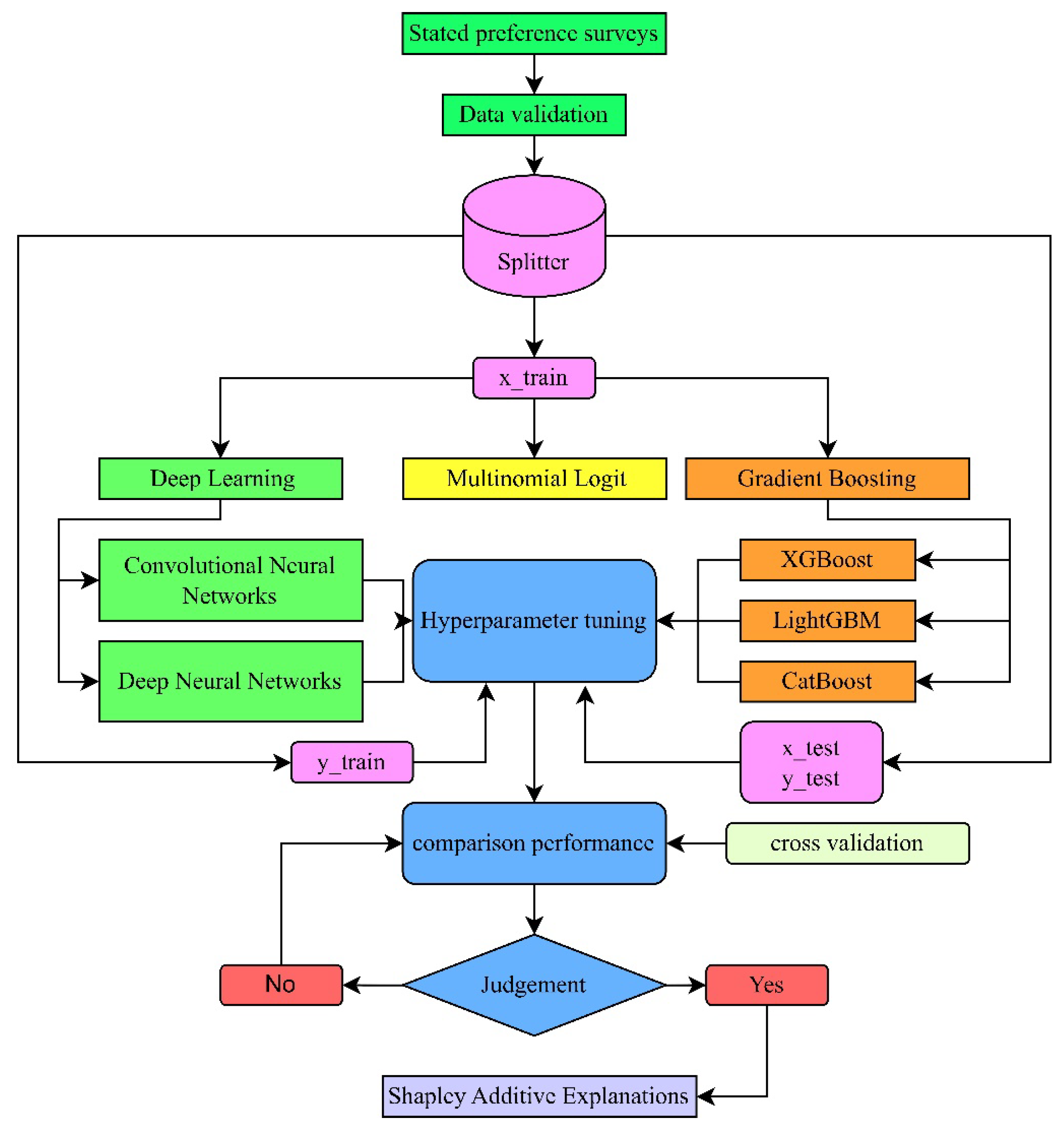
2.11. Model Comparison

To comprehensively conduct a comparative analysis of model effectiveness in identifying the key factors influencing the dependent variable (Y), this study explores the Multinomial Logit Model (MNL), Deep Neural Network (DNN), Convolutional Neural Network (CNN), Extreme Gradient Boosting (XGBoost), LightGBM, and CatBoost (Categorical Boosting). Given the diversity in modeling approaches, multiple evaluation metrics are employed to ensure a fair and robust comparison. To enhance the reliability and consistency of the assessment, a 10-fold cross-validation technique was applied to all models. This approach serves to attenuate overfitting and facilitates a more robust and generalizable assessment of model performance by systematically partitioning the dataset into distinct training and validation subsets. The comparative evaluation framework is anchored in three principal dimensions: predictive accuracy, model interpretability, and computational efficiency. With regard to predictive performance, the analysis underscores each model’s capacity to effectively capture the structural relationships between explanatory variables and the target outcome, rather than relying exclusively on conventional classification accuracy. To rigorously assess this dimension, a suite of strategically selected performance indicators is employed. In pursuit of a comprehensive appraisal of classification efficacy, this study adopts a multidimensional evaluation scheme that encapsulates a broader spectrum of diagnostic insights across model outputs. Rather than relying solely on classification accuracy, which may be insufficient in the presence of class imbalance, additional metrics are employed to capture different aspects of predictive performance. Accuracy serves as a general measure of correctly classified instances, while recall (sensitivity) and specificity provide insights into the model’s ability to correctly identify positive and negative cases, respectively. Furthermore, precision evaluates correctly predicted positives, while by integrating both precision and recall, the F1 score offers a single metric that reflects the model’s ability to maintain consistency between correct positive predictions and sensitivity, which is especially beneficial in skewed class distributions, especially for imbalanced datasets. The area under the ROC curve (AUC-ROC) is also used to evaluate the models’ ability to distinguish between different outcome categories. This metric is particularly valuable for multiclass classification, offering a threshold-independent assessment of performance. By applying these evaluation metrics uniformly across the Multinomial Logit Model (MNL), Deep Neural Network (DNN), Convolutional Neural Network (CNN), XGBoost, LightGBM, and CatBoost, this study ensures a robust and equitable comparison. This approach supports both the interpretability and predictive strength of each model in identifying the determinants of the dependent variable (Y).

Additionally, the area under the ROC curve (AUC-ROC) is employed to evaluate each model’s ability to distinguish between outcome classes across multiple prediction scenarios [29]. In parallel, accuracy is used as a baseline indicator for classification performance, quantifying the ratio of correct predictions to the overall number of cases. While accuracy is widely adopted, it is often augmented with supplementary metrics to address potential biases arising from class imbalance [29,45,58]. Considering the distinct methodological foundations of econometric versus machine learning techniques, the use of multiple evaluation criteria offers a more comprehensive and impartial basis for model comparison, capturing both interpretability and predictive reliability in estimating the determinants of the response variable.

Model performance was assessed using a set of evaluation metrics, including log loss, accuracy, precision, recall, and F1 score. To account for class imbalance and ensure uniform consideration across all outcome categories, macro-averaging was employed, thereby assigning equal weight to each class irrespective of its frequency [59,60].

$$\mathrm{A}\mathrm{c}\mathrm{c}\mathrm{u}\mathrm{r}\mathrm{a}\mathrm{c}\mathrm{y}={\displaystyle \frac{\mathrm{T}\mathrm{P}+\mathrm{T}\mathrm{N}}{\mathrm{T}\mathrm{P}+\mathrm{T}\mathrm{N}+\mathrm{F}\mathrm{P}+\mathrm{F}\mathrm{N}}}$$

(2)

$$\mathrm{R}\mathrm{e}\mathrm{c}\mathrm{a}\mathrm{l}\mathrm{l} (\mathrm{S}\mathrm{e}\mathrm{n}\mathrm{s}\mathrm{i}\mathrm{t}\mathrm{i}\mathrm{v}\mathrm{i}\mathrm{t}\mathrm{y})={\displaystyle \frac{\mathrm{T}\mathrm{P}}{\mathrm{T}\mathrm{P}+\mathrm{F}\mathrm{N}}}$$

(3)

$$\mathrm{S}\mathrm{p}\mathrm{e}\mathrm{c}\mathrm{i}\mathrm{f}\mathrm{i}\mathrm{c}\mathrm{i}\mathrm{t}\mathrm{y}={\displaystyle \frac{\mathrm{T}\mathrm{N}}{\mathrm{T}\mathrm{N}+\mathrm{F}\mathrm{P}}}$$

(4)

$$\mathrm{P}\mathrm{r}\mathrm{e}\mathrm{c}\mathrm{i}\mathrm{s}\mathrm{i}\mathrm{o}\mathrm{n}={\displaystyle \frac{\mathrm{T}\mathrm{P}}{\mathrm{T}\mathrm{P}+\mathrm{F}\mathrm{P}}}$$

(5)

$$\mathrm{F}-\mathrm{S}\mathrm{c}\mathrm{o}\mathrm{r}\mathrm{e}={\displaystyle \frac{2\mathrm{T}\mathrm{P}}{2\mathrm{T}\mathrm{P}+\mathrm{F}\mathrm{N}+\mathrm{F}\mathrm{P}}}$$

(6)

$$\mathrm{A}\mathrm{U}\mathrm{C}={\displaystyle \frac{1}{2}}(\mathrm{R}\mathrm{e}\mathrm{c}\mathrm{a}\mathrm{l}\mathrm{l}+\mathrm{S}\mathrm{p}\mathrm{e}\mathrm{c}\mathrm{i}\mathrm{f}\mathrm{i}\mathrm{c}\mathrm{i}\mathrm{t}\mathrm{y})$$

(7)

These performance metrics were derived from the confusion matrix, which summarizes the classification outcomes as follows:

TP (True Positive): instances where actual positives were accurately identified as positive;

TN (True Negative): instances where actual negatives were correctly recognized as negative;

FP (False Positive): cases in which negative instances were mistakenly classified as positive;

FN (False Negative): cases in which positive instances were wrongly labeled as negative.

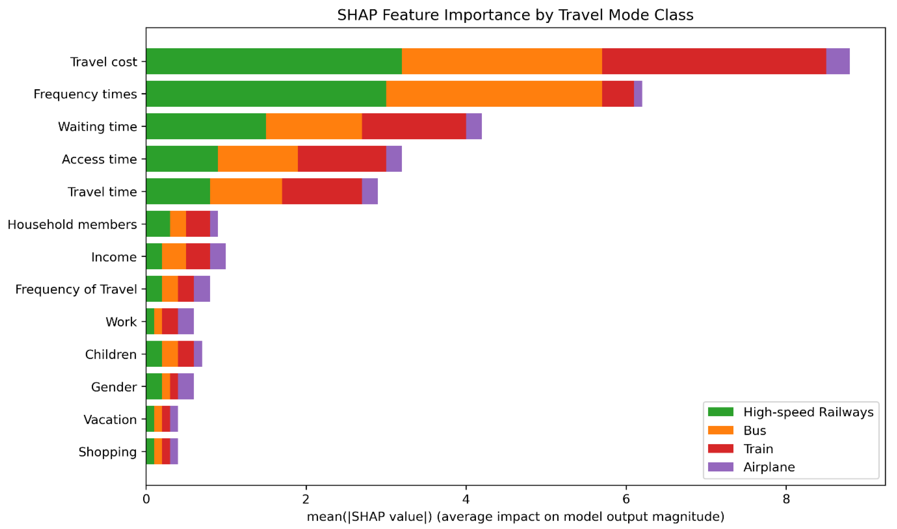
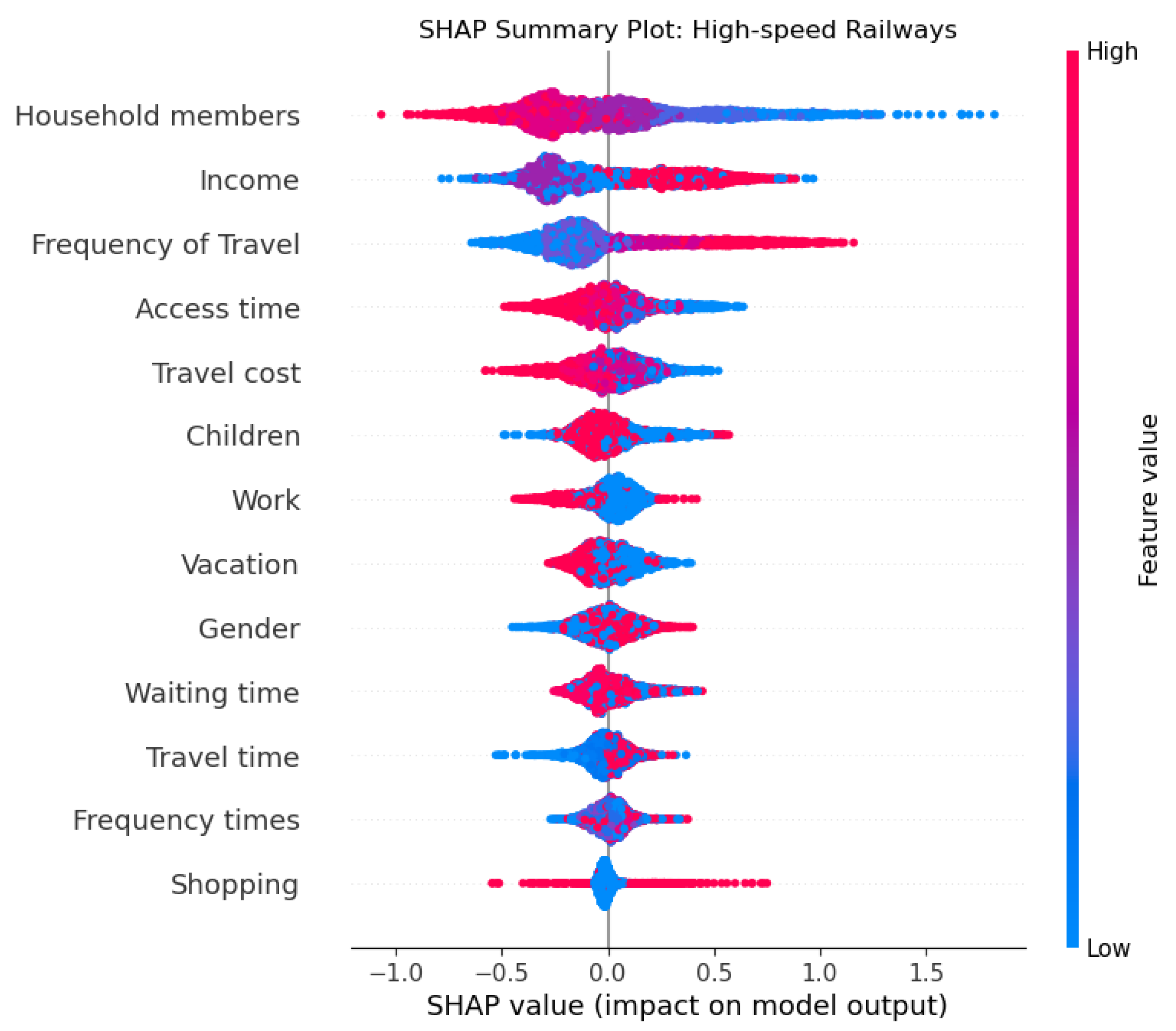
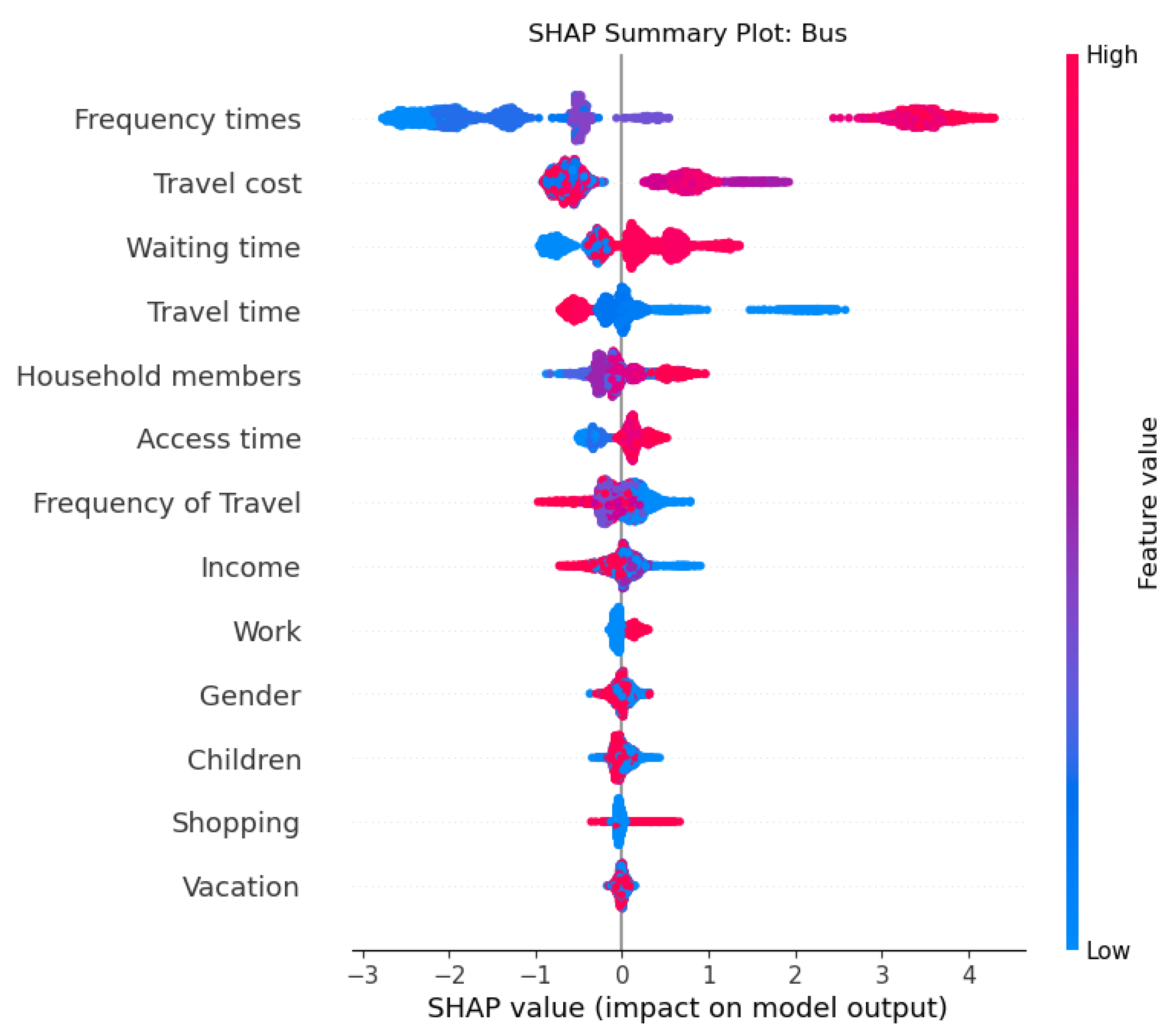
2.12. Shapley Additive Explanations (SHAP)

SHAP interprets complex machine learning models by showing how each feature influences predictions. It improves transparency and reliability through ranked plots, with position and color (red for positive, blue for negative) indicating each feature’s impact [61,62,63,64].

3. Results and Discussion

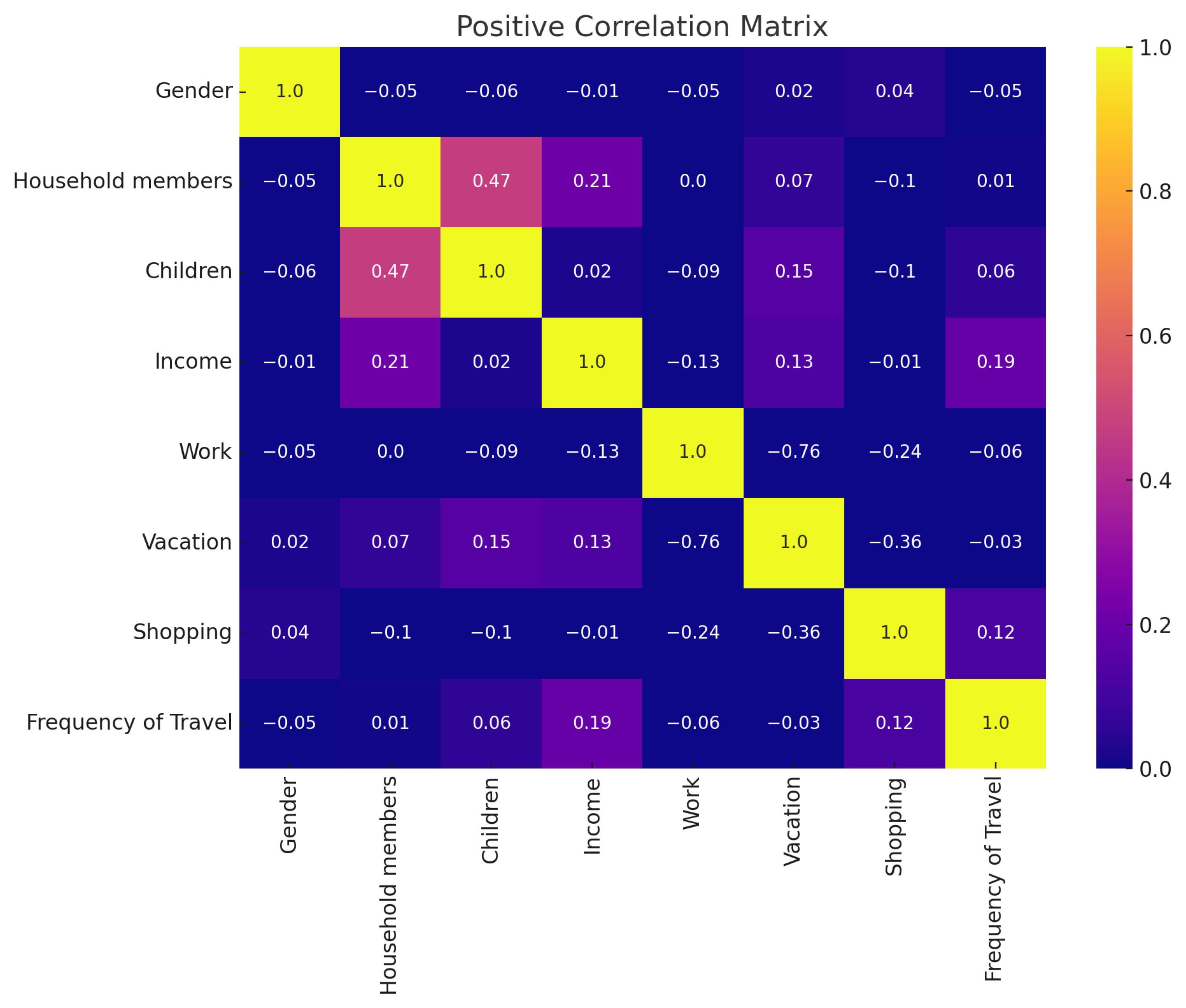
3.1. Descriptive Analysis

Below are the descriptive statistics for the key variables used in the analysis, including their distributions and summary measures relevant to the modeling process.

Table 2. Statistical Overview of Personal Characteristics and Mobility Behavior.

Variable	Description	Categorical Variable (%)	Mean	Standard Deviation	Skewness	Kurtosis
Gender	Male = 1	52.43	0.5243	0.4994	−0.0975	−1.9908
	Female = 0	47.57
	Total	100
Household members	Household members 1 person = 1	33.88	3.3561	1.1090	−0.3527	−0.5709
	2 people = 2	28.92
	3 people = 3	15.67
	4 people = 4	15.11
	More than four people = 5	6.41
	Total	100
Children	Have children under 18 in the household = 1	63.3	0.6330	0.4820	−0.5520	−1.6956
	No children under 18 in the household = 0	36.7
	Total	100
Income	Less than 15,000 = 1	2.22	2.9557	0.8705	−0.1163	−1.2520
	15,000–30,000 = 2	30.7
	30,001–45,000 = 3	33.54
	More than 45,000 = 4	33.55
	Total	100
Work	Travel for study or work. Yes = 1	33.39	0.3339	0.4716	0.7043	−1.5043
	No = 0	66.61
	Total	100
Vacation	Travel for leisure or vacation. Yes = 1	53.57	0.5357	0.4987	−0.1431	−1.9799
	No = 0	46.43
	Total	100
Shopping	Travel for shopping. Yes = 1	10.29	0.1029	0.3038	2.6146	4.837
	No = 0	89.71
	Total	100
Frequency of Travel	1–3 times = 1	35.72	2.1097	1.0673	0.5877	−0.9058
	3–6 times = 2	33.93
	6–9 times = 3	16.35
	More than nine times = 4	14
	Total	100
Mode	High speed railways = 1	29.42
	Bus = 2	27.45
	Train = 3	26.41
	Airplane = 4	16.72
	Total	100

summarizes the respondents’ sociodemographic and travel behavior characteristics. The sample consisted of 52.43% male and 47.57% female respondents. The average household size was 3.36 members, with single-person households being the most common (33.88%), followed by two-person households (28.92%). Regarding children under 18 in the household, 63.3% of respondents reported having children in this age group. In terms of household income, the majority of respondents had a monthly income in the range of 15,000 to 45,000 baht, with 33.55% earning more than 45,000 baht. The average income level (coded as categorical values) was 2.96. The most frequently reported travel purpose was for leisure or vacation (53.57%), followed by work or study (33.39%), and shopping (10.29%). The frequency of interprovincial travel averaged 2.11 times per month. Most respondents traveled one to three times per month (35.72%), while 33.93% reported traveling three to six times. In terms of mode choice, high-speed rail was the most preferred option, accounting for 29.42% of the responses, followed by bus (27.45%), conventional train (26.41%), and airplane (16.72%).

An examination of the skewness values across the variables showed a range between −0.55 and +0.70, indicating that most variables were approximately symmetrically distributed and did not display severe skewness. The kurtosis values were generally negative, suggesting that the distributions were flatter than the normal distribution [65].

To investigate the interrelationships among the explanatory variables and to assess potential multicollinearity, a Pearson correlation analysis was conducted. As shown in Figure 2, all pairwise correlation coefficients remain below the standard threshold of 0.5 [66], indicating that no substantial multicollinearity is present. The relatively low levels of intercorrelation confirm that the inclusion of these variables in a multivariate framework does not pose multicollinearity concerns, thereby validating the statistical independence required for reliable model estimation.

3.2. Hyperparameter Optimization Using Bayesian Optimization

In the development of high-performance predictive systems, hyperparameter optimization plays a pivotal role in enhancing model precision and generalizability. This consideration is particularly salient in the present study, which incorporates a diverse array of model architectures, including XGBoost, LightGBM, CatBoost, Deep Neural Network (DNN), and Convolutional Neural Network (CNN). Selecting optimal hyperparameter configurations is essential for maximizing model efficacy. Accordingly, this research utilizes Bayesian hyperparameter optimization, a probabilistic and data-efficient method for identifying optimal parameter settings under uncertainty. A summary of the optimized hyperparameter values for each algorithm is provided in

Table 3. Optimized Hyperparameters of the Compared Models.

Model	Description	Value
XGBoost	n_estimators	210
	max_depth	6
	learning_rate	0.21977629940065888
	subsample	0.8166577433928425
	colsample_bytree	0.6713509802187799
	gamma	0.016849547970738232
	reg_alpha	4.443653782167797
	reg_lambda	2.162026822349147
LightGBM	n_estimators	493
	max_depth	5
	learning_rate	0.0441
	subsample	0.8957
	colsample_bytree	0.9840
	reg_alpha	0.0754
	reg_lambda	0.0788
	random_state	42
CatBoost	iterations	157
	depth	7
	learning_rate	0.16214535070336702
	l2_leaf_reg	4.815982341211366
	random_strength	5.493473561258114
	bagging_temperature	0.5270768048053522
	border_count	113
	loss_function	‘MultiClass’
	random_state	42
Deep Neural Network	first_dense_units	191
	second_dense_units	87
	dropout_rate	0.2294
	optimizer	Adam
	learning_rate	0.00033001201097314586
	epochs	32
	batch_size	16
Convolutional Neural Network	filters	64
	kernel_size	3
	activation	‘relu’
	pool_size	2
	dense_units	64
	dropout_rate	0.3
	output_activation	‘softmax’
	optimizer	Adam
	learning_rate	0.001
	loss	‘categorical_crossentropy’
	batch_size	16
	epochs	30

.

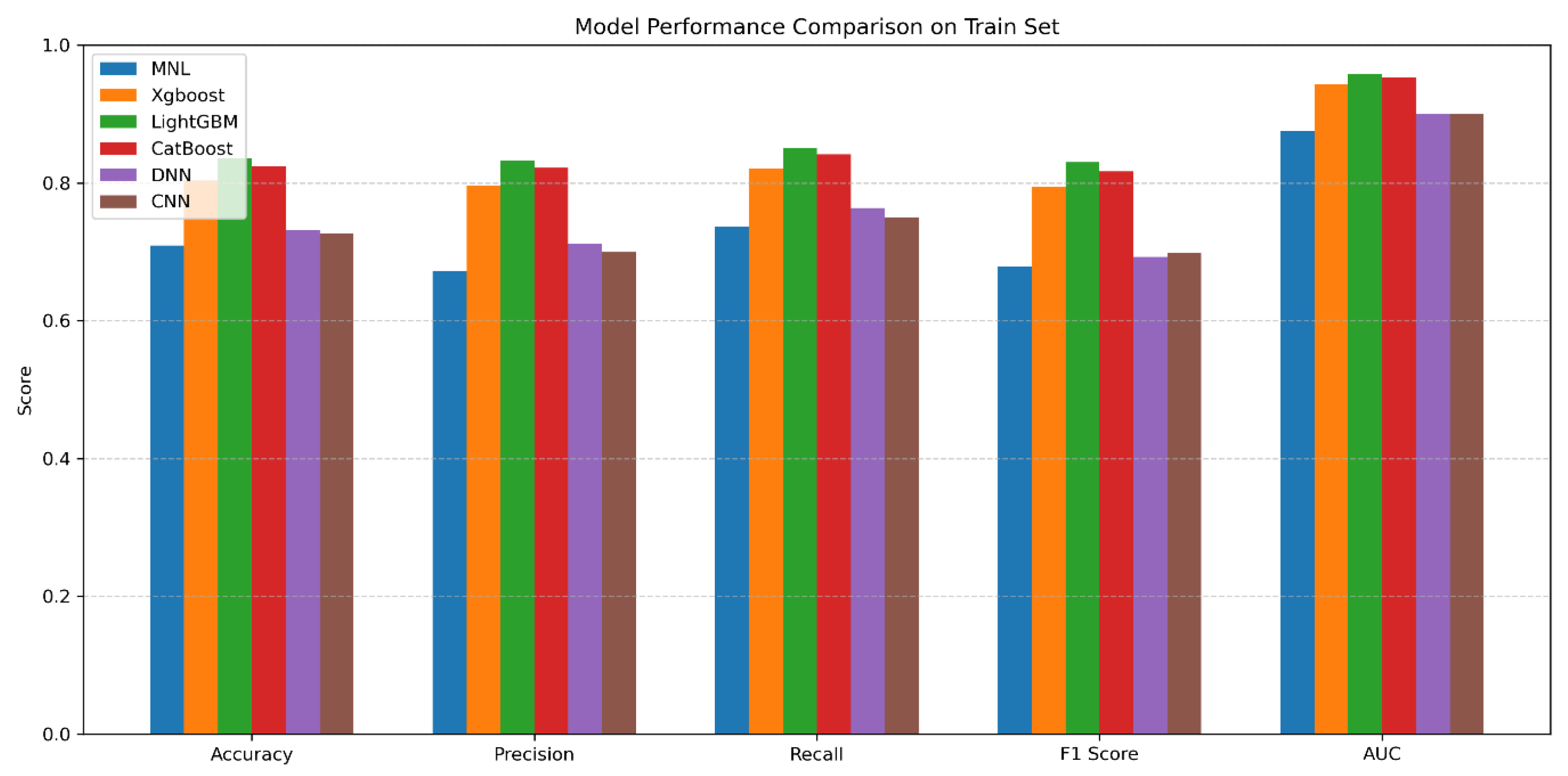
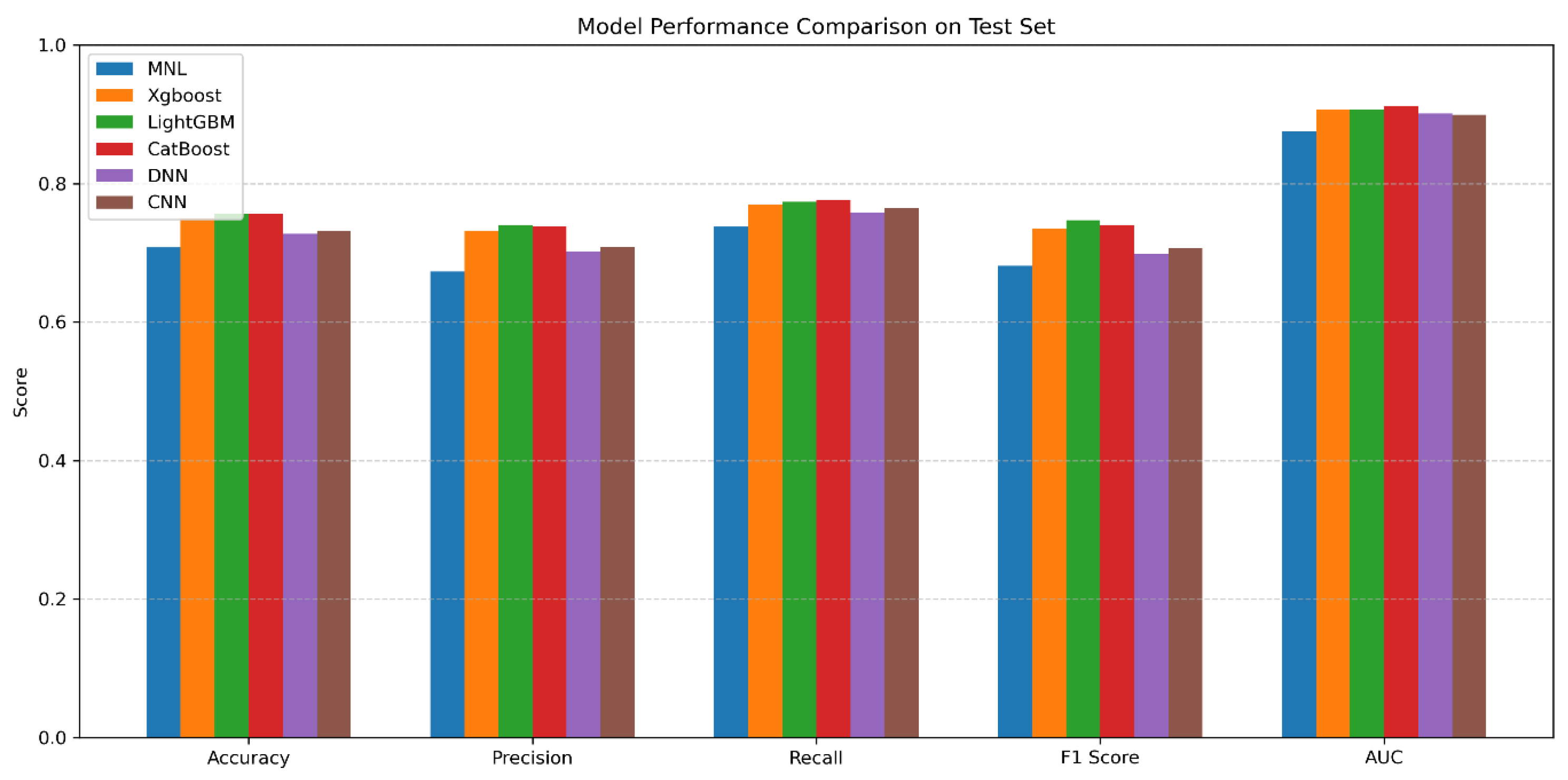
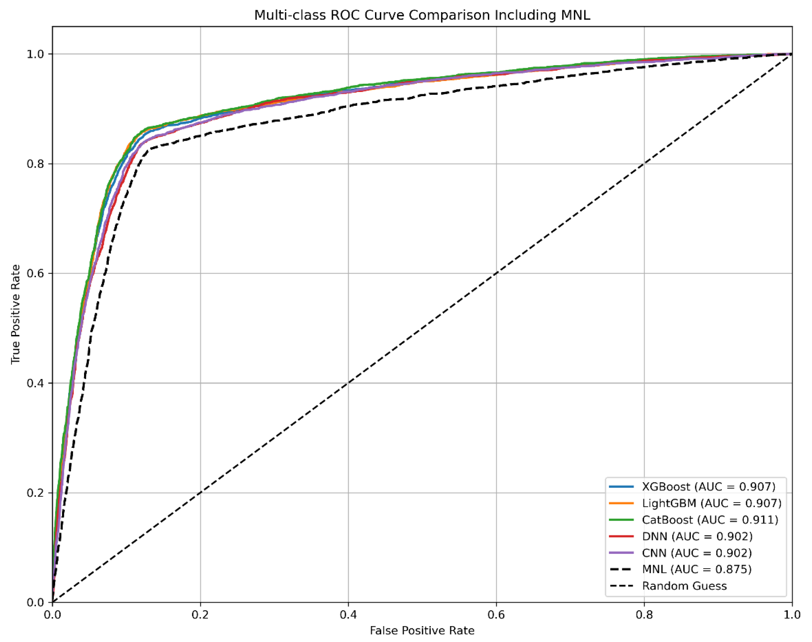
3.3. Model Performance

Model performance evaluation is critical for assessing the predictive accuracy of travel mode choice models, particularly in the context of promoting high-speed rail (HSR) as a competitive alternative to conventional transport modes such as buses, trains, and airplanes. To ensure methodological rigor and reduce sampling bias, a stratified 10-fold cross-validation procedure was employed, whereby the dataset was partitioned into ten mutually exclusive subsets. Each subset was sequentially designated as a validation set, while the remaining nine were used for model training, thereby enhancing the generalizability of the results. Key evaluation metrics—accuracy, precision, recall, F1 score (macro-averaged), and AUC for multiclass classification—were utilized to benchmark model performance. The outcomes are systematically presented in Figure 3 and Figure 4 to facilitate comparative analysis.

Figure 3 and Figure 4 present the cross-validated results for five predictive models—XGBoost, LightGBM, CatBoost, Deep Neural Network (DNN), and Convolutional Neural Network (CNN)—in forecasting travel mode transitions toward high-speed rail (HSR). Performance was assessed using standard classification metrics, including accuracy, precision, recall, F1 score, and area under the ROC curve (AUC), reported for both training and test sets to evaluate generalization capability.

Among the gradient boosting techniques, LightGBM achieved the highest scores on the training set, yielding peak values for accuracy (0.8355), F1 score (0.8299), and AUC (0.9584). Although CatBoost exhibited slightly lower training performance, it outperformed all models on the test set with the highest AUC (0.9113) and demonstrated consistent performance across all metrics—accuracy (0.7557), precision (0.7384), recall (0.7760), and F1 score (0.7404)—indicating robust generalization to unseen data.

The deep learning models (DNN and CNN) delivered stable yet slightly lower results on the test set, with accuracy and F1 scores ranging between 0.727 and 0.734, and comparatively reduced AUC values. Notably, the DNN model achieved the highest recall (0.7579), reflecting its sensitivity to correctly identifying positive cases.

In contrast, the Multinomial Logit (MNL) model underperformed across all evaluation criteria—accuracy (0.7081), precision (0.6731), recall (0.7373), F1 score (0.6812), and AUC (0.8753)—reflecting its limitations in handling nonlinearities and complex variable interactions. Despite its popularity in transport research for interpretability, MNL’s structural constraints limit its predictive accuracy. Overall, CatBoost emerged as the most effective model for HSR adoption prediction, striking the optimal balance between accuracy and generalization across all performance metrics.

Figure 5 illustrates the comparison of ROC curves across five classification models for predicting travel mode transitions toward high-speed rail (HSR) adoption. The CatBoost model achieved the highest macro-average AUC (0.911), followed closely by XGBoost and LightGBM (0.907), while DNN and CNN showed slightly lower but comparable performance (0.901 and 0.899, respectively). The results indicate that CatBoost demonstrates superior discriminatory power in differentiating among multiple travel mode classes. Only machine learning models are visualized in this figure, as the traditional Multinomial Logit (MNL) model showed substantially lower AUC and overall predictive performance, making it less effective for visual comparison.

The comparison of models in this study highlights significant performance differences across various approaches with distinct structures and assumptions. The Multinomial Logit (MNL) model, valued for its simplicity and behavioral interpretability, faces limitations due to its assumptions of linear relationships and the Independence of Irrelevant Alternatives (IIA), which hinder its ability to capture complex, nonlinear interactions [67]. As a result, MNL’s predictive performance, particularly in accuracy and AUC, was outperformed by machine learning (ML) models [68,69].

In contrast, machine learning models, particularly CatBoost, LightGBM, and XGBoost, exhibited significantly superior performance. These models excel at capturing complex variable interactions and can process categorical data directly, minimizing the need for extensive preprocessing [70]. Notably, CatBoost demonstrated particular strengths in addressing overfitting through integrated regularization mechanisms, which contributed to its robust accuracy and stability in the present dataset [65]. CatBoost utilizes ordered boosting (also known as ordered target statistics), which minimizes prediction shift during training and employs a symmetric tree-growing algorithm that promotes balanced and generalizable trees. Furthermore, its native handling of categorical variables through advanced encoding techniques allows for the preservation of essential information without manual transformation. The model also incorporates gradient-based regularization to enhance robustness, enabling it to perform well on structured datasets with minimal hyperparameter tuning [25,29,71].

Although Deep Neural Networks (DNNs) are capable of learning intricate, high-level data representations [72], their use on small datasets often leads to overfitting, as the number of parameters greatly exceeds the available data [73]. This leads the model to memorize training data rather than generalize underlying patterns, thereby reducing its effectiveness on unseen test data. Moreover, DNNs are susceptible to learning noise instead of meaningful structure [74]. Mitigating overfitting in such cases requires advanced techniques, including data augmentation, transfer learning, or other regularization strategies [75]. These complexities make the practical deployment of DNNs in small-data contexts challenging, where simpler models such as gradient boosting often outperform them. While Convolutional Neural Networks (CNNs) can technically be adapted for tabular data by arranging features into a matrix format resembling an image, thereby enabling the model to exploit spatial structure through convolutional filters, this approach may not be well suited in contexts where the features are inherently unordered and lack spatial correlation [76]. In the present study, the data were structured in a tabular format with semantically distinct and logically independent variables [77]. Therefore, convolutional learning was unable to extract salient features effectively [78]. While the deep learning models in this study, particularly DNN and CNN, were constrained by the limited sample size, several strategies were employed to mitigate overfitting and enhance generalization. Although the original sample consisted of 3200 respondents, the stated preference (SP) design included 12 hypothetical choice tasks per person, resulting in a dataset of 38,400 observations. This enriched dataset allowed for more effective model training despite the moderate respondent base. To further address overfitting, we implemented stratified 10-fold cross-validation, Bayesian hyperparameter tuning, and incorporated dropout layers and early stopping during the training of DNN and CNN models. These regularization techniques aimed to reduce model complexity and prevent memorization of the training data. In contrast, models tailored for tabular data—such as CatBoost and XGBoost—demonstrated greater efficiency in handling categorical variables without preprocessing and capturing nonlinear patterns, resulting in higher accuracy and more stable performance on this dataset [32,76,79].

Figure 6 presents the SHAP-based global feature importance analysis, offering key insights into the relative influence of individual factors driving the shift in travel mode choices, particularly toward the adoption of high-speed rail (HSR). The results emphasize that economic and temporal service characteristics play a far more dominant role than sociodemographic attributes in shaping travelers’ decision-making processes. Travel cost emerges as the most influential factor across all travel modes, particularly in the context of airplane and bus choices. This underscores the high price sensitivity among travelers, especially in low-to-middle-income contexts like Thailand, where affordability remains a crucial determinant in mode selection [48,80,81]. This finding aligns with established transport economics theory, which identifies cost as a central constraint in mode choice decisions [81,82].

Beyond cost, service frequency and waiting time emerge as key determinants, especially among train and bus users. These results suggest that operational predictability and schedule reliability are key considerations for travelers [83,84]. Low service frequency and prolonged waiting times pose substantial barriers to HSR adoption, reinforcing the need for strategic interventions to enhance service regularity [85]. This reflects the concept of perceived temporal utility, where delays and inconsistencies in departure or arrival times reduce the perceived value of the service. Travelers tend to associate high-frequency services with lower opportunity costs and greater flexibility, which enhances the attractiveness of the mode. Access time and travel time, representing components of total journey effort, show moderate SHAP values across modes. Their consistent influence across all alternatives highlights their importance in overall convenience, particularly for users with limited access to HSR stations [86,87]. This is consistent with the theory of generalized travel cost, which incorporates not only monetary cost but also time-related burdens such as first-mile/last-mile travel and in-vehicle duration. Inadequate access and long travel times increase the perceived disutility of HSR, especially for travelers who value efficiency or have time constraints.

In contrast, sociodemographic variables—household size, income, gender, and trip purpose—show comparatively low SHAP importance. This indicates that mode choice is driven more by service characteristics than by traveler attributes, a trend that diverges from traditional behavioral models that emphasize demographics [88,89]. Although variables like income are commonly used in travel behavior studies, the current results reveal that actual trip cost has a more direct and substantial impact on decision-making than income levels. Nonetheless, variables such as travel frequency and gender, though ranked lower, retain non-zero SHAP values, suggesting latent behavioral patterns. For instance, regular travelers may prioritize punctuality and convenience more heavily, increasing their likelihood of shifting to HSR when reliability is perceived to be superior [90]. This finding implies that frequent intercity travelers such as commuters, business travelers, or students who travel regularly between provinces represent a key target segment for early HSR adoption. These groups are often time-sensitive and more responsive to improvements in service frequency and travel time, making them ideal candidates for tailored marketing strategies and service design.

In summary, the SHAP analysis confirms the primacy of economic and temporal attributes notably cost, service frequency, and waiting time in determining mode shifts toward HSR. These findings have direct implications for transportation policy and service design, underscoring the need to enhance affordability and reliability to foster greater adoption of HSR systems. In addition, the results highlight specific passenger groups—such as frequent travelers, larger households, and higher-income individuals—who exhibit greater sensitivity to improvements in HSR-related service attributes. These segments represent strategic targets for early adoption and should be prioritized in marketing, fare policy, and service design to maximize uptake and long-term viability.

The disaggregated SHAP analysis by travel mode reveals a distinctive behavioral pattern among high-speed rail (HSR) users (Figure 7), in which household size emerges as a prominent determinant. This effect is not observed in the other transport modes. Moreover, income demonstrates contrasting influences: individuals with higher income levels show a greater propensity to choose HSR, while their likelihood of using bus services declines. These findings suggest a clear socioeconomic differentiation in travel mode preferences.

Across all four transport modes (HSR, bus, train, and airplane), travel cost and time-related service attributes, including service frequency, waiting time, and access time, consistently emerge as the most influential factors in shaping mode choice. These variables exert particularly strong effects among bus and train users (Figure 8 and Figure 9), highlighting the critical importance of operational efficiency and schedule reliability. In the case of air travel (Figure 10), access time and cost are especially salient, indicating heightened sensitivity to first- and last-mile connectivity as well as fare levels in mode selection.

These findings underscore the policy importance of enhancing affordability and temporal reliability in HSR service design. Tailored strategies such as competitive fare structures, increased service frequency, and improved station accessibility are vital to promoting HSR adoption. Moreover, targeted incentives for specific user segments, such as larger households and higher-income travelers, may further enhance the attractiveness of HSR in emerging intercity transport systems.

4. Conclusions

This study compared the predictive performance of traditional and advanced modeling techniques in forecasting travel mode choice amid the introduction of high-speed rail (HSR) in Thailand. Using stated preference data from diverse geographic and socioeconomic contexts, the analysis evaluated the Multinomial Logit (MNL) model alongside advanced models including Extreme Gradient Boosting, LightGBM, CatBoost, Deep Neural Networks (DNNs), and Convolutional Neural Networks (CNNs), with model training enhanced through cross-validation and Bayesian optimization. The proposed modeling framework not only demonstrates strong predictive performance in the context of Thailand’s HSR, but also holds potential for application in similar large-scale transportation infrastructure studies across different countries or systems. CatBoost achieved the highest performance on the test set, with an AUC of 0.9113 and an accuracy of 0.7557, demonstrating superior generalization compared to all other models. While LightGBM obtained the highest training AUC of 0.9584, CatBoost maintained more stable performance on unseen data, attributed to its algorithmic features such as native handling of categorical variables and ordered boosting. The MNL model, although interpretable and easy to implement, was constrained by structural assumptions like linearity and the Independence of Irrelevant Alternatives (IIA), resulting in a lower AUC of 0.8753. Deep learning models (DNN and CNN) showed limited performance due to data volume constraints and the mismatch between CNN architecture and tabular data structure.

Feature importance analysis using SHAP revealed that travel cost, service frequency, and waiting time were the most influential factors in mode choice, particularly for bus and air travel. In contrast, sociodemographic variables had limited impact, indicating that service attributes play a more dominant role in shaping HSR-related travel decisions. Although this study did not perform an explicit segmentation analysis, the results suggest certain passenger groups are more likely to adopt high-speed rail services. In particular, travelers with higher income levels, larger households, and those who travel frequently for business or educational purposes demonstrate greater sensitivity to HSR’s economic and temporal attributes. These findings point to the practical value of targeting such groups in future marketing and service planning efforts, especially during the early stages of HSR implementation.

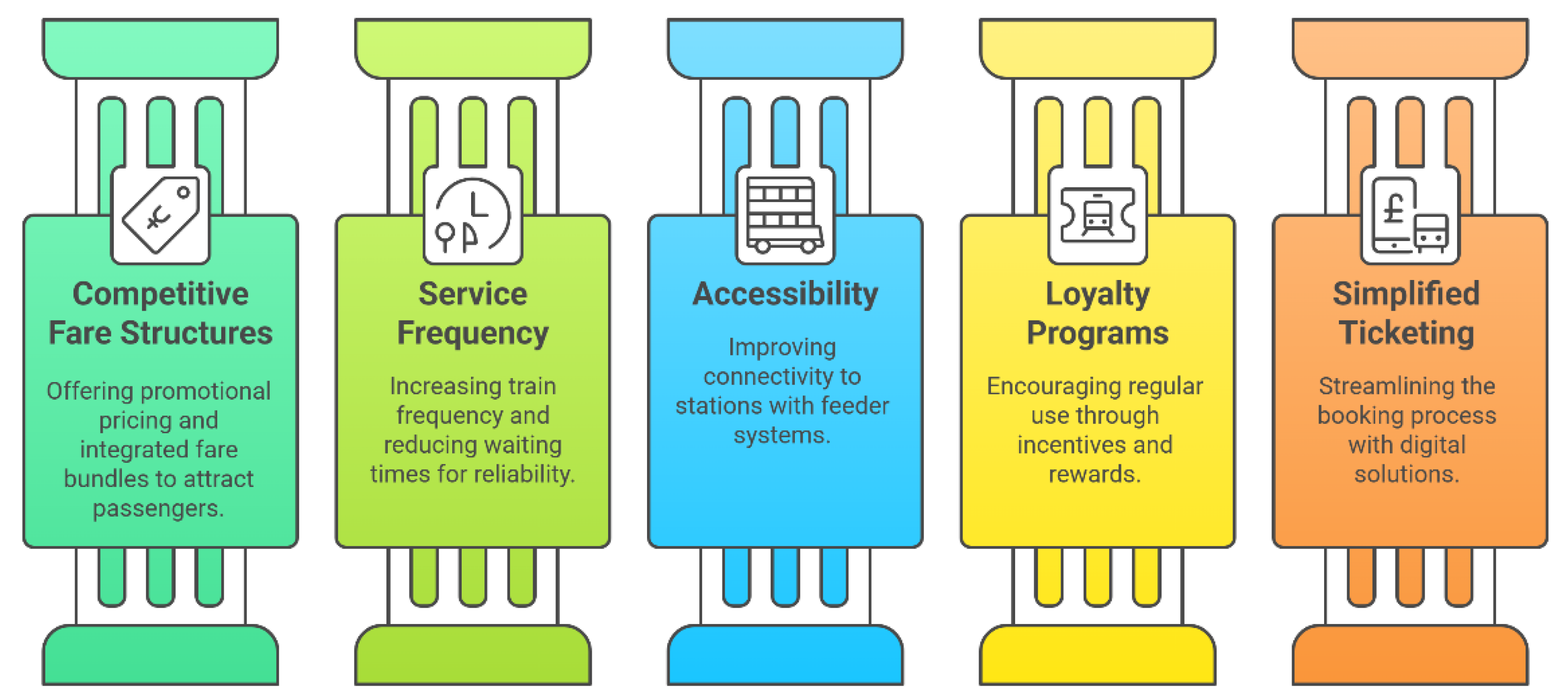
4.1. Policy Recommendations

Informed by the empirical findings, this study proposes the following policy recommendations to promote the adoption of high-speed rail, as depicted in Figure 11:

• Design competitive fare structures by offering promotional pricing, monthly passes, or integrated fare bundles with other public transportation services;
• Increase service frequency and minimize waiting times to enhance the reliability and attractiveness of high-speed rail operations;
• Improve accessibility to rail stations through feeder systems such as shuttle buses or local transit networks that facilitate first-mile and last-mile connectivity;
• Encourage regular intercity travelers to adopt high-speed rail through loyalty programs or targeted fare incentives;
• Simplify the ticketing process by developing a seamless and intuitive platform for booking and payment, supporting mobile access, QR code usage, and electronic wallets.

In conclusion, this study demonstrates not only the superior predictive performance of machine learning models, especially Categorical Boosting, in modeling travel mode choice but also underscores the critical role of service-related attributes in influencing behavioral shifts. These insights provide a practical foundation for designing efficient, inclusive, and user-centered transportation policies, particularly in the context of high-speed rail development in Thailand and other emerging economies.

4.2. Limitations and Further Research

This study provides valuable insights into travel mode choice behavior in the context of high-speed rail (HSR) development in Thailand. However, several limitations should be acknowledged. First, the use of stated preference (SP) data introduces potential hypothetical bias, as respondents’ stated intentions under hypothetical scenarios may not align with their actual behavior. This is especially relevant for emerging systems like HSR, for which respondents have no prior experience. Future research should incorporate revealed preference (RP) data following real-world implementation to validate model predictions. In addition, future studies may consider developing multiple hypothetical travel scenarios and evaluating different predictive targets beyond mode choice, such as user satisfaction, likelihood of repeated use, or pricing sensitivity.

Second, although advanced machine learning and deep learning models were employed, the modest dataset size may have limited the performance of complex architectures, particularly Deep Neural Networks (DNNs) and Convolutional Neural Networks (CNNs), which are typically optimized for large-scale data. Despite the use of cross-validation and hyperparameter tuning, these models may still be prone to overfitting. Expanding the dataset and employing techniques such as transfer learning or ensemble methods may enhance performance in future studies.

Third, the study utilized a non-probability sampling approach, which, despite ensuring regional coverage, may limit the generalizability of the results due to potential selection bias. Future research should adopt stratified or probability-based sampling techniques to ensure more representative and externally valid conclusions.

Fourth, the models do not explicitly account for latent psychological constructs such as attitudes, perceptions, or satisfaction, which are increasingly recognized as key determinants of travel behavior. This unexpectedly weak influence of demographic variables may be attributed to specific cultural characteristics in Thailand, where travel decisions are more influenced by practical constraints (e.g., cost and access) than personal traits. Additionally, limitations in the questionnaire design may have restricted the ability to capture attitudinal or psychological dimensions that mediate the effect of sociodemographic factors. Incorporating latent variable modeling techniques such as hybrid choice models or Structural Equation Modeling (SEM) could improve explanatory power.

Fifth, while Shapley Additive Explanations (SHAP) was used to interpret global feature importance, this method does not account for temporal dynamics or context-specific variability. Future work should consider longitudinal data and time series modeling to capture behavioral adaptation following HSR implementation. In addition, future research could extend SHAP analysis by incorporating interaction effects between key service attributes such as travel cost, waiting time, and service frequency to uncover how combinations of factors jointly influence mode choice decisions. This would provide deeper behavioral insights beyond individual variable importance. Cross-country comparative studies, particularly in other developing nations, may also offer valuable insights into the transferability and generalizability of machine learning approaches in travel behavior research. Moreover, future studies could extend SHAP analysis by incorporating interaction effects among key variables, such as cost, waiting time, and service frequency. Assessing these combined influences may reveal compound sensitivities that are not apparent when considering each factor in isolation. Additionally, clustering algorithms or latent class analysis could be applied to segment travelers into subgroups—such as budget-sensitive, time-sensitive, or frequent users—and assess model performance and behavioral responses within each cluster. These segmentation techniques would allow for more targeted policy recommendations and service planning based on distinct traveler profiles.

Finally, future research should explore traveler segmentation techniques such as clustering, latent class analysis, or subgroup-specific modeling to uncover distinct user profiles and heterogeneity in preferences. This would allow for more tailored policy interventions and service strategies that address the unique needs of different passenger groups, such as frequent travelers, students, or price-sensitive individuals.

References

1. Liang, Y.; Zhou, K.; Li, X.; Zhou, Z.; Sun, W.; Zeng, J. Effectiveness of high-speed railway on regional economic growth for less developed areas. J. Transp. Geogr. 2020, 82, 102621. [Google Scholar] [CrossRef]
2. Blanquart, C.; Koning, M. The local economic impacts of high-speed railways: Theories and facts. Eur. Transp. Res. Rev. 2017, 9, 12. [Google Scholar] [CrossRef]
3. Wu, W.; Liang, Y.; Wu, D. Evaluating the impact of China’s rail network expansions on local accessibility: A market potential approach. Sustainability 2016, 8, 512. [Google Scholar] [CrossRef]
4. Tissayakorn, K. A Study on Transit-Oriented Development Strategies in the High-Speed Rail Project in Thailand. Ph.D. Thesis, Yokohama National University, Yokohama, Japan, 2021. [Google Scholar]
5. Office of the National Economic and Social Development Council. Sustainable Development Goals: SDGs. Available online: https://sdgs.nesdc.go.th/goals-and-indicators/ (accessed on 30 January 2023).
6. State Railway of Thailand. High-Speed Rail Route Between Bangkok and Nong Khai (Phase 2: Nakhon Ratchasima to Nong Khai). Available online: https://www.hsrkorat-nongkhai.com/ (accessed on 30 January 2023).
7. JTTRI-AIRO. Progress of the Thailand-China High-Speed Railway. 2023. Available online: https://www.jttri-airo.org/en/dll.php?id=20&s=pdf1&t=repo (accessed on 3 February 2023).
8. Yang, W.; Chen, Q.; Yang, J. Factors Affecting Travel Mode Choice between High-Speed Railway and Road Passenger Transport—Evidence from China. Sustainability 2022, 14, 15745. [Google Scholar] [CrossRef]
9. Deng, Y.; Bai, Y.; Cui, L.; He, R. Travel Mode Choice Behavior for High-Speed Railway Stations Based on Multi-Source Data. Transp. Res. Rec. 2023, 2677, 525–540. [Google Scholar] [CrossRef]
10. Wang, J.; Zhao, W.; Liu, C.; Huang, Z. A System Optimization Approach for Trains’ Operation Plan with a Time Flexible Pricing Strategy for High-Speed Rail Corridors. Sustainability 2023, 15, 9556. [Google Scholar] [CrossRef]
11. Liu, L.; Zhang, M. High-speed rail impacts on travel times, accessibility, and economic productivity: A benchmarking analysis in city-cluster regions of China. J. Transp. Geogr. 2018, 73, 25–40. [Google Scholar] [CrossRef]
12. Zhang, Y.; Liang, K.; Yao, E.; Gu, M. Measuring Reliable Accessibility to High-Speed Railway Stations by Integrating the Utility-Based Model and Multimodal Space–Time Prism under Travel Time Uncertainty. ISPRS Int. J. Geo-Inf. 2024, 13, 263. [Google Scholar] [CrossRef]
13. Zhou, Y.; Zhao, M.; Tang, S.; Lam, W.H.; Chen, A.; Sze, N.; Chen, Y. Assessing the relationship between access travel time estimation and the accessibility to high speed railway station by different travel modes. Sustainability 2020, 12, 7827. [Google Scholar] [CrossRef]
14. Ben-Akiva, M.E.; Lerman, S.R. Discrete Choice Analysis: Theory and Application to Travel Demand; MIT Press: Cambridge, MA, USA, 1985; Volume 9. [Google Scholar]
15. Török, Á.; Szalay, Z.; Uti, G.; Verebélyi, B. Rerepresenting autonomated vehicles in a macroscopic transportation model. Period. Polytech. Transp. Eng. 2020, 48, 269–275. [Google Scholar] [CrossRef]
16. Akter, T.; Alam, B.M. Travel mode choice behavior analysis using multinomial logit models towards creating sustainable college campus: A case study of the University of Toledo, Ohio. Front. Future Transp. 2024, 5, 1389614. [Google Scholar] [CrossRef]
17. Ning, J.; Lyu, T.; Wang, Y. Exploring the built environment factors in the metro that influence the ridership and the market share of the elderly and students. J. Adv. Transp. 2021, 2021, 9966794. [Google Scholar] [CrossRef]
18. Wen, C.-H.; Wang, W.-C.; Fu, C. Latent class nested logit model for analyzing high-speed rail access mode choice. Transp. Res. Part E Logist. Transp. Rev. 2012, 48, 545–554. [Google Scholar] [CrossRef]
19. Wu, J.; Yang, M.; Sun, S.; Zhao, J. Modeling travel mode choices in connection to metro stations by mixed logit models: A case study in Nanjing, China. Promet-Traffic Transp. 2018, 30, 549–561. [Google Scholar] [CrossRef]
20. Kwigizile, V.; Chimba, D.; Sando, T. A cross-nested logit model for trip type-mode choice: An application. Adv. Transp. Stud. 2011, 29–40. [Google Scholar]
21. Bierlaire, M. A theoretical analysis of the cross-nested logit model. Ann. Oper. Res. 2006, 144, 287–300. [Google Scholar] [CrossRef]
22. Hasnine, M.S.; Lin, T.; Weiss, A.; Habib, K.N. Determinants of travel mode choices of post-secondary students in a large metropolitan area: The case of the city of Toronto. J. Transp. Geogr. 2018, 70, 161–171. [Google Scholar] [CrossRef]
23. Chen, T.; Guestrin, C. Xgboost: A scalable tree boosting system. In Proceedings of the 22nd ACM Sigkdd International Conference on Knowledge Discovery and Data Mining, San Francisco, CA, USA, 13–17 August 2016; pp. 785–794. [Google Scholar]
24. Ke, G.; Meng, Q.; Finley, T.; Wang, T.; Chen, W.; Ma, W.; Ye, Q.; Liu, T.-Y. Lightgbm: A highly efficient gradient boosting decision tree. Adv. Neural Inf. Process. Syst. 2017, 3149–3157. [Google Scholar]
25. Prokhorenkova, L.; Gusev, G.; Vorobev, A.; Dorogush, A.V.; Gulin, A. CatBoost: Unbiased boosting with categorical features. Adv. Neural Inf. Process. Syst. 2018, 6639–6649. [Google Scholar]
26. Abulibdeh, A. Analysis of mode choice affects from the introduction of Doha Metro using machine learning and statistical analysis. Transp. Res. Interdiscip. Perspect. 2023, 20, 100852. [Google Scholar] [CrossRef]
27. Díaz-Ramírez, J.; Estrada-García, J.A.; Figueroa-Sayago, J. Predicting transport mode choice preferences in a university district with decision tree-based models. City Environ. Interact. 2023, 20, 100118. [Google Scholar] [CrossRef]
28. Wen, X.; Chen, X. A New Breakthrough in Travel Behavior Modeling Using Deep Learning: A High-Accuracy Prediction Method Based on a CNN. Sustainability 2025, 17, 738. [Google Scholar] [CrossRef]
29. Banyong, C.; Hantanong, N.; Wisutwattanasak, P.; Champahom, T.; Theerathitichaipa, K.; Seefong, M.; Ratanavaraha, V.; Jomnonkwao, S. A machine learning comparison of transportation mode changes from high-speed railway promotion in Thailand. Results Eng. 2024, 24, 103110. [Google Scholar] [CrossRef]
30. Guo, L.; Huang, J.; Ma, W.; Sun, L.; Zhou, L.; Pan, J.; Yang, W. Convolutional Neural Network-Based Travel Mode Recognition Based on Multiple Smartphone Sensors. Appl. Sci. 2022, 12, 6511. [Google Scholar] [CrossRef]
31. Hillel, T.; Bierlaire, M.; Elshafie, M.Z.E.B.; Jin, Y. A systematic review of machine learning classification methodologies for modelling passenger mode choice. J. Choice Model. 2021, 38, 100221. [Google Scholar] [CrossRef]
32. Grinsztajn, L.; Oyallon, E.; Varoquaux, G. Why do tree-based models still outperform deep learning on typical tabular data? Adv. Neural Inf. Process. Syst. 2022, 35, 507–520. [Google Scholar]
33. Dahmen, V.; Weikl, S.; Bogenberger, K. Interpretable machine learning for mode choice modeling on tracking-based revealed preference data. Transp. Res. Rec. 2024, 2678, 2075–2091. [Google Scholar] [CrossRef]
34. Office of the National Economic and Social Development Council. Gross Regional and Provincial Product Chain Volume Measure 2022 Edition. Available online: https://www.nesdc.go.th/nesdb_en/ewt_dl_link.php?nid=4317/ (accessed on 1 December 2024).
35. Srithongrung, A.; Kriz, K.A. Thai Public Capital Budget and Management Process. In Capital Management and Budgeting in the Public Sector; IGI Global: Hershey, PA, USA, 2019; pp. 206–235. [Google Scholar]
36. Pavlou, M.; Ambler, G.; Qu, C.; Seaman, S.R.; White, I.R.; Omar, R.Z. An evaluation of sample size requirements for developing risk prediction models with binary outcomes. BMC Med. Res. Methodol. 2024, 24, 146. [Google Scholar] [CrossRef]
37. Kujala, R.; Weckström, C.; Mladenović, M.N.; Saramäki, J. Travel times and transfers in public transport: Comprehensive accessibility analysis based on Pareto-optimal journeys. Comput. Environ. Urban Syst. 2018, 67, 41–54. [Google Scholar] [CrossRef]
38. Arencibia, A.I.; Feo-Valero, M.; García-Menéndez, L.; Román, C. Modelling mode choice for freight transport using advanced choice experiments. Transp. Res. Part A Policy Pract. 2015, 75, 252–267. [Google Scholar] [CrossRef]
39. Economic Base. Knock on the Bangkok-Chiang Mai High-Speed Train Fare 1089 Baht. Available online: https://www.thansettakij.com/business/242231 (accessed on 4 February 2023).
40. BusOnlineTicket.co.th. Book Thailand Bus Tickets Online. Available online: https://www.busonlineticket.co.th/ (accessed on 3 February 2023).
41. AirAsia Move. Flight. Available online: https://www.airasia.com/th/th (accessed on 6 February 2023).
42. State Railway of Thailand the State Railway of Thailand Easy Book, Convenient Check. Available online: https://dticket.railway.co.th/DTicketPublicWeb/home/Home (accessed on 7 February 2023).
43. Hensher, D.A.; Rose, J.M.; Greene, W.H. Applied Choice Analysis; Cambridge University Press: Cambridge, UK, 2015. [Google Scholar]
44. García-Ródenas, R.; Linares, L.J.; López-Gómez, J.A. On the performance of classic and deep neural models in image recognition. In Proceedings of the Artificial Neural Networks and Machine Learning–ICANN 2017: 26th International Conference on Artificial Neural Networks, Alghero, Italy, 11–14 September 2017; Proceedings, Part II 26. pp. 600–608. [Google Scholar]
45. García-García, J.C.; García-Ródenas, R.; López-Gómez, J.A.; Martín-Baos, J.Á. A comparative study of machine learning, deep neural networks and random utility maximization models for travel mode choice modelling. Transp. Res. Procedia 2022, 62, 374–382. [Google Scholar] [CrossRef]
46. Xu, Y.; Zhao, X.; Chen, Y.; Yang, Z. Research on a mixed gas classification algorithm based on extreme random tree. Appl. Sci. 2019, 9, 1728. [Google Scholar] [CrossRef]
47. Krizhevsky, A.; Sutskever, I.; Hinton, G.E. Imagenet classification with deep convolutional neural networks. Commun. ACM 2012, 60, 84–90. [Google Scholar] [CrossRef]
48. Li, X.; Shi, L.; Shi, Y.; Tang, J.; Zhao, P.; Wang, Y.; Chen, J. Exploring interactive and nonlinear effects of key factors on intercity travel mode choice using XGBoost. Appl. Geogr. 2024, 166, 103264. [Google Scholar] [CrossRef]
49. Friedman, J.H. Greedy function approximation: A gradient boosting machine. Ann. Stat. 2001, 29, 1189–1232. [Google Scholar] [CrossRef]
50. Ding, C.; Cao, X.J.; Næss, P. Applying gradient boosting decision trees to examine non-linear effects of the built environment on driving distance in Oslo. Transp. Res. Part A Policy Pract. 2018, 110, 107–117. [Google Scholar] [CrossRef]
51. Elith, J.; Leathwick, J.R.; Hastie, T. A working guide to boosted regression trees. J. Anim. Ecol. 2008, 77, 802–813. [Google Scholar] [CrossRef]
52. Dorogush, A.V.; Ershov, V.; Gulin, A. CatBoost: Gradient boosting with categorical features support. arXiv 2018, arXiv:1810.11363. [Google Scholar]
53. Zhai, W.; Li, C.; Fei, S.; Liu, Y.; Ding, F.; Cheng, Q.; Chen, Z. CatBoost algorithm for estimating maize above-ground biomass using unmanned aerial vehicle-based multi-source sensor data and SPAD values. Comput. Electron. Agric. 2023, 214, 108306. [Google Scholar] [CrossRef]
54. Pham, T.D.; Yokoya, N.; Xia, J.; Ha, N.T.; Le, N.N.; Nguyen, T.T.T.; Dao, T.H.; Vu, T.T.P.; Pham, T.D.; Takeuchi, W. Comparison of machine learning methods for estimating mangrove above-ground biomass using multiple source remote sensing data in the red river delta biosphere reserve, Vietnam. Remote Sens. 2020, 12, 1334. [Google Scholar] [CrossRef]
55. Huang, G.; Wu, L.; Ma, X.; Zhang, W.; Fan, J.; Yu, X.; Zeng, W.; Zhou, H. Evaluation of CatBoost method for prediction of reference evapotranspiration in humid regions. J. Hydrol. 2019, 574, 1029–1041. [Google Scholar] [CrossRef]
56. Chongzhi, W.; Lin, W.; Zhang, W. Chapter 14—Assessment of undrained shear strength using ensemble learning based on Bayesian hyperparameter optimization. In Modeling in Geotechnical Engineering; Samui, P., Kumari, S., Makarov, V., Kurup, P., Eds.; Academic Press: Cambridge, MA, USA, 2021; pp. 309–326. [Google Scholar]
57. Shakya, A.; Biswas, M.; Pal, M. Chapter 9—Classification of Radar data using Bayesian optimized two-dimensional Convolutional Neural Network. In Radar Remote Sensing; Srivastava, P.K., Gupta, D.K., Islam, T., Han, D., Prasad, R., Eds.; Elsevier: Amsterdam, The Netherlands, 2022; pp. 175–186. [Google Scholar]
58. Zhao, X.; Yan, X.; Yu, A.; Van Hentenryck, P. Modeling Stated preference for mobility-on-demand transit: A comparison of Machine Learning and logit models. arXiv 2018, arXiv:1811.01315. [Google Scholar]
59. Mokhtarimousavi, S.; Anderson, J.C.; Azizinamini, A.; Hadi, M. Factors affecting injury severity in vehicle-pedestrian crashes: A day-of-week analysis using random parameter ordered response models and artificial neural networks. Int. J. Transp. Sci. Technol. 2020, 9, 100–115. [Google Scholar] [CrossRef]
60. Sokolova, M.; Lapalme, G. A systematic analysis of performance measures for classification tasks. Inf. Process. Manag. 2009, 45, 427–437. [Google Scholar] [CrossRef]
61. Mangalathu, S.; Hwang, S.-H.; Jeon, J.-S. Failure mode and effects analysis of RC members based on machine-learning-based SHapley Additive exPlanations (SHAP) approach. Eng. Struct. 2020, 219, 110927. [Google Scholar] [CrossRef]
62. Mao, H.; Deng, X.; Jiang, H.; Shi, L.; Li, H.; Tuo, L.; Shi, D.; Guo, F. Driving safety assessment for ride-hailing drivers. Accident Anal. Prev. 2021, 149, 105574. [Google Scholar] [CrossRef]
63. Adland, R.; Jia, H.; Lode, T.; Skontorp, J. The value of meteorological data in marine risk assessment. Reliab. Eng. Syst. Saf. 2021, 209, 107480. [Google Scholar] [CrossRef]
64. Vega, G.M.; Aznarte José, L. Shapley additive explanations for NO2 forecasting. Ecol. Inform. 2020, 56, 101039. [Google Scholar] [CrossRef]
65. Champahom, T.; Banyong, C.; Hantanong, N.; Se, C.; Jomnonkwao, S.; Ratanavaraha, V. Factors influencing the willingness to pay for motorcycle safety improvement: A structural equation modeling approach. Transp. Res. Interdiscip. Perspect. 2023, 22, 100950. [Google Scholar] [CrossRef]
66. Vatcheva, K.P.; Lee, M.; McCormick, J.B.; Rahbar, M.H. Multicollinearity in regression analyses conducted in epidemiologic studies. Epidemiology 2016, 6, 227. [Google Scholar] [CrossRef]
67. Kalantari, H.A.; Sabouri, S.; Brewer, S.; Ewing, R.; Tian, G. Machine Learning in Mode Choice Prediction as Part of MPOs’ Regional Travel Demand Models: Is It Time for Change? Sustainability 2025, 17, 3580. [Google Scholar] [CrossRef]
68. Shahdah, U.E.; Elharoun, M.; Ali, E.K.; Elbany, M.; Elagamy, S.R. Stated preference survey for predicting eco-friendly transportation choices among Mansoura University students. Innov. Infrastruct. Solut. 2025, 10, 180. [Google Scholar] [CrossRef]
69. Yin, C.; Wu, J.; Sun, X.; Meng, Z.; Lee, C. Road transportation emission prediction and policy formulation: Machine learning model analysis. Transp. Res. Part D Transp. Environ. 2024, 135, 104390. [Google Scholar] [CrossRef]
70. Yu, J.; Chang, X.; Hu, S.; Yin, H.; Wu, J. Combining travel behavior in metro passenger flow prediction: A smart explainable Stacking-Catboost algorithm. Inf. Process. Manag. 2024, 61, 103733. [Google Scholar] [CrossRef]
71. Chen, H.; Cheng, Y. Travel mode choice prediction using imbalanced machine learning. IEEE Trans. Intell. Transp. Syst. 2023, 24, 3795–3808. [Google Scholar] [CrossRef]
72. Zhang, C.; Bengio, S.; Hardt, M.; Recht, B.; Vinyals, O. Understanding deep learning (still) requires rethinking generalization. Commun. ACM 2021, 64, 107–115. [Google Scholar] [CrossRef]
73. Himeur, Y.; Elnour, M.; Fadli, F.; Meskin, N.; Petri, I.; Rezgui, Y.; Bensaali, F.; Amira, A. Next-generation energy systems for sustainable smart cities: Roles of transfer learning. Sustain. Cities Soc. 2022, 85, 104059. [Google Scholar] [CrossRef]
74. Li, M.; Soltanolkotabi, M.; Oymak, S. Gradient descent with early stopping is provably robust to label noise for overparameterized neural networks. In Proceedings of the International Conference on Artificial Intelligence and Statistics, Online, 26 August 2020; pp. 4313–4324. [Google Scholar]
75. Fort, S.; Dziugaite, G.K.; Paul, M.; Kharaghani, S.; Roy, D.M.; Ganguli, S. Deep learning versus kernel learning: An empirical study of loss landscape geometry and the time evolution of the neural tangent kernel. Adv. Neural Inf. Process. Syst. 2020, 33, 5850–5861. [Google Scholar]
76. Shwartz-Ziv, R.; Armon, A. Tabular data: Deep learning is not all you need. Inf. Fusion 2022, 81, 84–90. [Google Scholar] [CrossRef]
77. Chehreh Chelgani, S.; Homafar, A.; Nasiri, H.; Rezaei laksar, M. CatBoost-SHAP for modeling industrial operational flotation variables—A “conscious lab” approach. Miner. Eng. 2024, 213, 108754. [Google Scholar] [CrossRef]
78. Kadra, A.; Lindauer, M.; Hutter, F.; Grabocka, J. Well-tuned simple nets excel on tabular datasets. Adv. Neural Inf. Process. Syst. 2021, 34, 23928–23941. [Google Scholar]
79. Borisov, V.; Leemann, T.; Seßler, K.; Haug, J.; Pawelczyk, M.; Kasneci, G. Deep neural networks and tabular data: A survey. IEEE Trans. Neural Netw. Learn. Syst. 2024, 35, 7499–7519. [Google Scholar] [CrossRef] [PubMed]
80. Chen, P.; Zhang, X.; Gao, D. Preference heterogeneity analysis on train choice behaviour of high-speed railway passengers: A case study in China. Transp. Res. Part A Policy Pract. 2024, 188, 104198. [Google Scholar] [CrossRef]
81. Xu, M.; Shuai, B.; Wang, X.; Liu, H.; Zhou, H. Analysis of the accessibility of connecting transport at High-speed rail stations from the perspective of departing passengers. Transp. Res. Part A Policy Pract. 2023, 173, 103714. [Google Scholar] [CrossRef]
82. Salas, P.; De la Fuente, R.; Astroza, S.; Carrasco, J.A. A systematic comparative evaluation of machine learning classifiers and discrete choice models for travel mode choice in the presence of response heterogeneity. Expert Syst. Appl. 2022, 193, 116253. [Google Scholar] [CrossRef]
83. Wahab, S.N.; Hamzah, M.I.; Suki, N.M.; Chong, Y.S.; Kua, C.P. Unveiling passenger satisfaction in rail transit through a consumption values perspective. Multimodal Transp. 2025, 4, 100196. [Google Scholar] [CrossRef]
84. Grolle, J.; Donners, B.; Annema, J.A.; Duinkerken, M.; Cats, O. Service design and frequency setting for the European high-speed rail network. Transp. Res. Part A Policy Pract. 2024, 179, 103906. [Google Scholar] [CrossRef]
85. Tiong, K.Y.; Ma, Z.; Palmqvist, C.-W. Analyzing factors contributing to real-time train arrival delays using seemingly unrelated regression models. Transp. Res. Part A Policy Pract. 2023, 174, 103751. [Google Scholar] [CrossRef]
86. Moyano, A.; Moya-Gómez, B.; Gutiérrez, J. Access and egress times to high-speed rail stations: A spatiotemporal accessibility analysis. J. Transp. Geogr. 2018, 73, 84–93. [Google Scholar] [CrossRef]
87. Zhou, Z.; Cheng, L.; Yang, M.; Wang, L.; Chen, W.; Gong, J.; Zou, J. Analysis of passenger perception heterogeneity and differentiated service strategy for air-rail intermodal travel. Travel Behav. Soc. 2024, 37, 100872. [Google Scholar] [CrossRef]
88. Romero, C.; Zamorano, C.; Monzón, A. Exploring the role of public transport information sources on perceived service quality in suburban rail. Travel Behav. Soc. 2023, 33, 100642. [Google Scholar] [CrossRef]
89. Zhou, H.; Chi, X.; Norman, R.; Zhang, Y.; Song, C. Tourists’ urban travel modes: Choices for enhanced transport and environmental sustainability. Transp. Res. Part D Transp. Environ. 2024, 129, 104144. [Google Scholar] [CrossRef]
90. Chen, Z. Socioeconomic Impacts of high-speed rail: A bibliometric analysis. Socio-Econ. Plan. Sci. 2023, 85, 101265. [Google Scholar] [CrossRef]
Figure 1. Research process flowchart.
Bdcc 09 00155 g001
Figure 2. Heatmap of positive correlation among socioeconomic factors.
Bdcc 09 00155 g002
Figure 3. Model performance comparison on the training set.
Bdcc 09 00155 g003
Figure 4. Model performance comparison on the test set.
Bdcc 09 00155 g004
Figure 5. Multiclass ROC curve comparison across models including Multinomial Logit.
Bdcc 09 00155 g005
Figure 6. SHAP feature importance disaggregated by travel mode class.
Bdcc 09 00155 g006
Figure 7. SHAP feature importance and impact on high-speed rail mode choice.
Bdcc 09 00155 g007
Figure 8. SHAP feature importance and impact on bus mode choice.
Bdcc 09 00155 g008
Figure 9. SHAP feature importance and impact on train mode choice.
Bdcc 09 00155 g009
Figure 10. SHAP feature importance and impact on airplane mode choice.
Bdcc 09 00155 g010
Figure 11. Enhancing high-speed rail adoption through strategic policy recommendations.
Bdcc 09 00155 g011