Abstract
Nitrogen is one of the most important macronutrients for crops, and, in conjunction with artificial intelligence algorithms, it is possible to estimate it with the aid of vegetation indices through remote sensing. Various indices were calculated and those with a correlation of ≥0.7 were selected for subsequent use in random forest, gradient boosting, and artificial neural networks to determine their relationship with nitrogen levels measured in the laboratory. Random forest showed no relationship, yielding an R2 of zero; and gradient boosting and the classical method were similar with 0.7; whereas artificial neural networks yielded the best results with an R2 of 0.93. Thus, estimating nitrogen levels using this algorithm is reliable, by feeding it with data from the Modified Chlorophyll Absorption Ratio Index, Transformed Chlorophyll Absorption Reflectance Index, Modified Chlorophyll Absorption Ratio Index/Optimized Soil Adjusted Vegetation Index, and Transformed Chlorophyll Absorption Ratio Index/Optimized Soil Adjusted Vegetation Index
1. Introduction
Fig (Ficus carica) is a crop of Mediterranean origin that is of great economic importance due to its fruit and nutritional quality [1]. Mexico is currently one of the main fig producers in the world, producing 11,500 tons in 2022 [2]. And this trend is expected to continue, since recent studies indicate that the transverse neo-volcanic axis, western Sierra Madre, and north–central Mexico have suitable habitats for fig production in future years under conditions of climate change [3].
Fig trees can survive in nutrient-poor conditions; however, it does not mean that they are not necessary [4]. Nitrogen in plants is the most important macronutrient in agroecosystems, as it participates in crucial biochemical reactions involved in plant physiology, development, growth, and yield, as well as in the nutritional contribution to crop fruits [5,6]. Visually, nitrogen deficiencies are characterized by leaf chlorosis, flower drop, stunting, and plant senescence [7], although these deficiencies manifest late.
In the study conducted by [8] on nutrient deficiency in fig crops, it was found that a nitrogen deficiency causes almost no growth, with a low number of leaves, generalized chlorosis, and sparse foliage, as well as plants with a stunted and yellowish appearance, while an excess causes a delayed ripening of the fruits, which affects their quality [4].
Remote sensing is a technique that allows us to obtain information about terrestrial objects from a distance [9]; in agriculture, it allows us to classify crops and helps us to understand the phenological state of each crop through spectral signatures and vegetation indices [10], which are tools that provide fast, relevant, and non-destructive information, resulting from combinations of the spectral bands recorded by satellites. Their function is to measure several variables such as chlorophyll, biomass, and leaf area index, among others [11,12], thus allowing the early identification of nutritional deficiencies, such as nitrogen, which can be detected based on chlorophyll reflectance, since more than 50% of the nitrogen is used in the photosynthetic apparatus; therefore, photosynthesis is affected by nitrogen availability [13,14].
Indices, such as those belonging to the CARI family, reduce the variability of photosynthetically active radiation due to the presence of various non-photosynthetic materials. The Modified Chlorophyll Absorption Ratio Index (MCARI) is a measure of the depth of chlorophyll absorption at 670 nm relative to the reflectance at 550 and 700 nm, and the Transformed Chlorophyll Absorption Ratio Index (TCARI) measures the depth of chlorophyll absorption in the red relative to the maximum peaks of reflectance at the green and red edge—it is very sensitive to soil reflectivity, so it is combined with the Optimized Soil Adjusted Vegetation Index (OSAVI) to minimize soil background effects [15,16].
Artificial intelligence (AI) is a discipline within computer science that deals with the design and construction of systems capable of performing tasks related to human intelligence, thus focusing on the use of machine-learning (ML) techniques [17,18], which are a subset of artificial intelligence methods that allow machines to learn from experience [19]. Within machine-learning algorithms, stacking, bagging, and boosting predominate [20].
Stacking combines heterogeneous weak learners using a meta-learning model to improve the prediction accuracy through two phases: first, different models are learned from an original training dataset using top-level learners, and then these models are combined to constitute the training data for meta-learning, creating a new dataset to obtain the final result [21,22,23]; bagging reduces the variance in prediction through random sampling by combining multiple estimates from different models, providing a more stable result and helping to overcome the problems of a limited sample size [20,21], while boosting provides sequential learning: the first learner is trained on the initial dataset, while subsequent learners try to improve on previous errors, which means it attempts to reduce bias by sequentially fitting multiple homogeneous weak learners [18,21].
These AI techniques have gained momentum in agriculture in recent years, especially when combined with satellite imagery, as they streamline various methodologies with predictive results. In recent years, there have been advances in land use and vegetation classification [24], biomass estimation [25], and pest and nutrient detection in soil and plants [26]. In addition, there have been advances in nitrogen prediction for agricultural production [27]. Since the determination of nitrogen in plants by the Kjeldahl method, which is the most widely used, requires a plant sample, which is time-consuming, the objective of the present study was to estimate the nitrogen content in fig crops using remote sensing and machine-learning algorithms during their phenological development, with which deficiencies of this macronutrient could be solved before there are major problems.
2. Materials and Methods
2.1. Study Area
The study area is located in northern Mexico, in the region known as “La Comarca Lagunera” in the state of Durango, with co-ordinates of 25°34′12″ north latitude and 103°29′47″ west longitude, at an altitude ranging between 1100 and 1800 m above sea level. The climate in the region is very dry and semi-warm, with an average annual precipitation of 250 mm, while the annual average temperature ranges between 18 °C and 22 °C [28,29].
2.2. Description and Characterization of Field Work
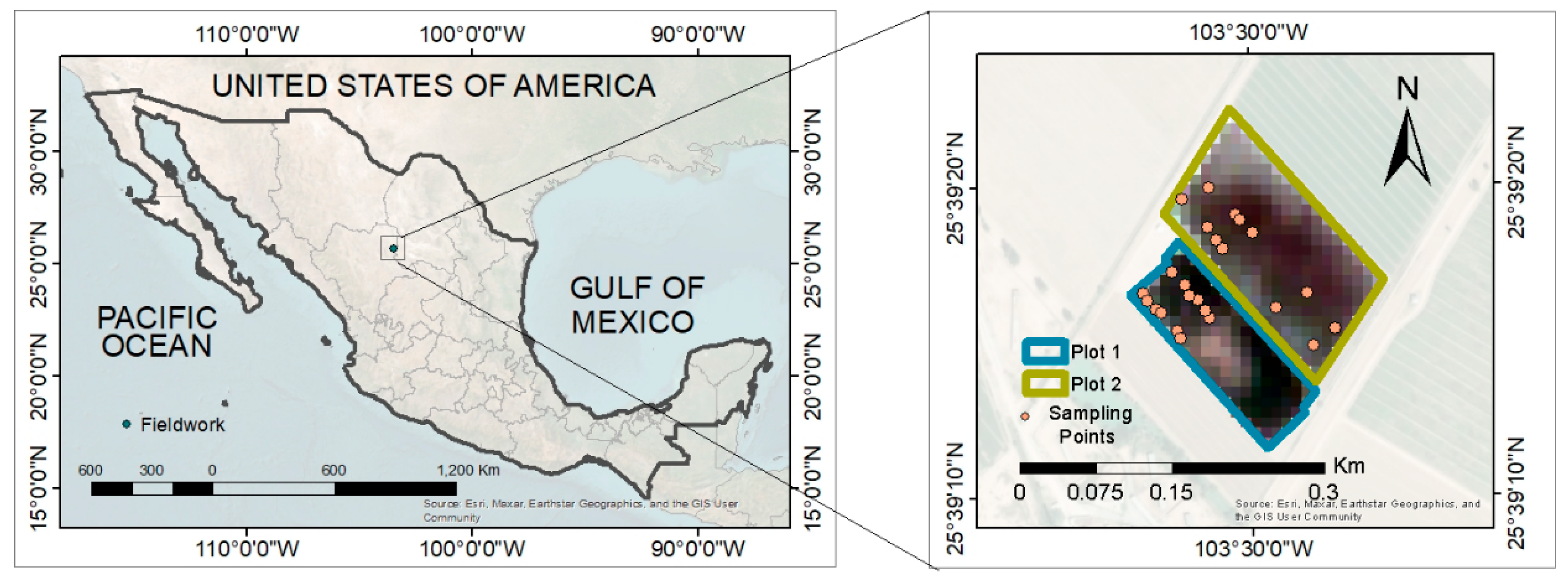
The work was carried out in the agricultural area of Ana’s Farm, in the El Vergel community, with co-ordinates 25°39′16″ north latitude and 103°29′55″ west longitude (Figure 1), with an altitude of 1120 m above sea level and a slope of 10%. Two plots were selected, one of them with 15-year-old fig trees under drip irrigation (Plot 1), and the second plot with 10-year-old trees under gravity irrigation (Plot 2). Two sampling points were selected from each plot, and, within each point, six subsamples were randomly selected to consider repetitions. Agricultural management, such as tree pruning, irrigation, and fertilization, was carried out by the farm.
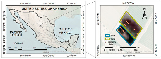
Figure 1.
Geographical location of Ana’s Farm in northern Mexico.
For soil characterization of the site, three samplings were performed at the beginning, middle, and end of the 2022 production cycle. A zigzag sampling was performed at a depth of 0–30, then a composite subsample was made with three replicates of each plot for subsequent laboratory analysis. Analyses were determined in the soil laboratory of the Technological Institute of Torreon, following the protocols of NOM-021-SEMART-2000, with results presented in Table 1.

Table 1.
Soil characterization of the study area at the beginning (April), middle (August), and end October) of the 2022 production cycle.
Foliar sampling was conducted every 10 days, coinciding with the passage of the Sentinel-2 satellite. From each sampling point (selected trees), the actively photosynthesizing leaf (young and fully expanded) corresponding to each cardinal point was taken and stored in a cooler to be later transported to the Technological Institute of Torreon for chlorophyll determination. This was carried out using the method proposed by Lichtenthaler (1987) [30] through spectroscopy, which utilizes fresh samples for the determination of chlorophyll a, chlorophyll b, and carotenoids in ppm, whereas, for foliar nitrogen, the Kjeldahl method was employed.
2.3. Satellital Images and Index Data
Satellite images corresponding to each of the sampled days (Julian days 107, 117, 130, 137, 147, 157, 177, 201, 217, 228, 257, 272, 287, and 297) were downloaded from Sentinel-2 sensor of the Copernicus Open Access Hub platform (https://scihub.copernicus.eu/dhus/#/home; accessed on 2 April 2022), discarding those with a high percentage of cloud cover (107 and 157). The selected images were standardized in size and pixel number. According to several authors such as Salvador-Castillo et al. (2021) and Feng et al. (2022) [31,32], various spectral indices can be used to estimate nitrogen, which, for the present study, were calculated using ArcGIS software ver. 10.8 [33]. Additionally, indices from the VICAL platform (https://inifapcenidraspa.users.earthengine.app/view/vical; accessed on 30 October 2022) developed by Jiménez-Jiménez et al. (2022) [34] were included.
2.4. Index Selected
The data of the obtained indices (Table 2) were extracted from each sampling point, and, through Pearson correlation analysis (p ≤ 0.05), the relationship between these indices and the nitrogen value calculated through laboratory analysis was visualized. Using R software ver. 4.0, indices with a correlation coefficient ≥0.7 with nitrogen were selected.

Table 2.
Selected spectral indices for nitrogen determination.
2.5. Artificial Intelligence Models
Artificial neural networks (ANNs) are based on biological neural networks, mimicking the functioning of neurons in the human brain [40,41]. They consist of a series of units called nodes or artificial neurons, arranged in layers; each neuron is connected to others through communication links, and each is assigned a value that the network uses to solve a specific problem [42].
The most basic ANN is the perceptron or single-layer network, but it has limitations, such as the inability to separate regions that are not linearly separable [42]. The multi-layer perceptron (MLP), known as a multi-layer perceptron network, is widely preferred within the family of neural networks because of its ability to represent both simple and complex functional relationships [43]. Its key features include its high nonlinearity, fault tolerance, ability to establish relationships between datasets, and suitability for hardware implementations [44].
For the artificial neural network, “resilient backpropagation” was used, through which, on discovering the first failure at the original location, the algorithm is able to backtrack and signal anomalies affecting both the nodes and the previous layers.
Two hidden layers with an array 5.3 were used with a “threshold” value of 0.05 for the partial derivatives of the error function as a stopping criterion. The “max_step” parameter was set to 1 × 10⁷, and the “rep” to one for network training. The logistic function was used to smooth the result of the cross product of the covariate or neurons and the weights.
Random forest (RF) is a more complex version of bagging, introduced by Breiman in 2001, being a supervised learning technique that generates multiple decision trees on a training dataset [45,46]. This methodology uses two essential parameters, the number of trees and the number of predictors to use in each split of each tree, with the advantage of being a simpler model to train compared to others, but with similar results, as well as maintaining its accuracy even with large portions of missing data; however, it is more difficult to interpret [45,47].
For random forest, regression was used with the parameters “keep_forest” to keep the output object, number of trees “ntree” set to 500, and “mtry” set to two, which is the number of predictors to be randomly sampled at each split when building the tree models. The parameter “importance” was taken into account for the generation of a matrix in which the first column represents the average decrease in precision, and the second column represents the average decrease in mean square error.
Gradient boosting, gradient tree boosting, or gradient-boosted regression trees (GBRTs), is a family of algorithms used for classification and regression based on the combination of weak predictive models (weak learners), which are individual decision trees that are adjusted to the negative gradient of the binomial or multinomial deviance loss function, where numerical predictors are handled as categorical without having to create indicator variables; in other words, each new tree tries to improve errors from the previous trees [20,48]. The parameters for the realization of this methodology were: distribution = “gaussian”, cv.folds = 10, shrinkage = 0.01, n.minobsinnode = 10, and n.trees = 500.
2.6. Data Validation
To improve non-parametric regression methods, it is necessary to carry out a learning process using training data. These data are used to build a model in which parameters are adjusted to minimize estimation error. In this case, the k-fold cross-validation method with five subsets was employed to evaluate the performance of predictive models. This method has been used to validate various learning models, such as random forest, neural networks, and gradient boosting. The technique involves dividing the dataset into two subsets, one for training and the other for validation. In this study, 70% of the data was allocated for training or fitting, and the remaining 30% for validation [49].
To optimize model performance, it is essential to adjust key hyperparameters such as n_estimators and max_features. During the training phase, different combinations of these hyperparameters are tested to achieve the best possible performance. However, there is a risk of overfitting the data, so k-fold cross-validation is used [50]. In this process, the dataset is divided into two subsets: training and validation. Then, in the k-fold method, the training set is divided into five subsets (Figure 2) using only the training set for this purpose. This means that five independent training models are created to validate the model, and the average of these five accuracies will be the final accuracy.
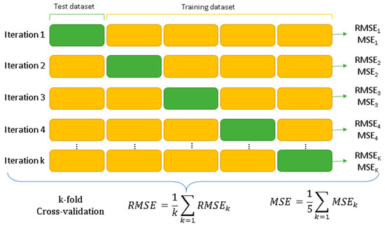
Figure 2.
Schematization of k-fold cross-validation [51].
Figure 2.
Schematization of k-fold cross-validation [51].
2.7. Model Performance Evaluation
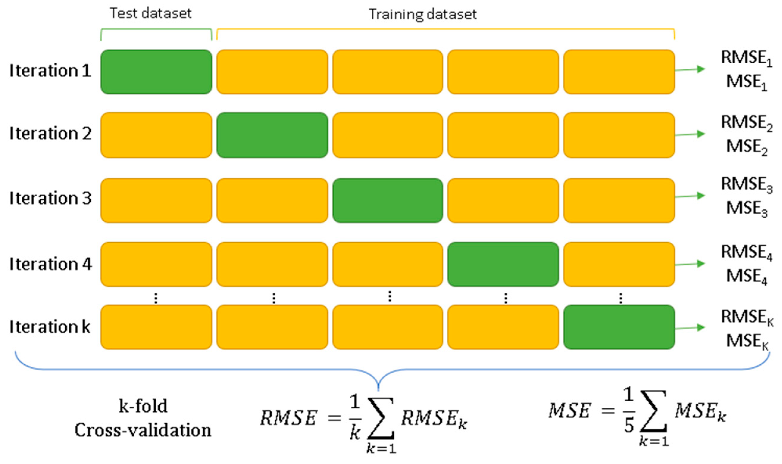
To evaluate the performance in nitrogen estimation, the coefficient of determination (R2), root mean squared error (RMSE), and mean squared error (MSE) were used, with the following formulae:
where, Oi, Si, , , and n represent the observed data, the estimated data, the mean value of the observed data, the mean value of the estimated data, and the number of samples, respectively.
3. Results
3.1. Lab Nitrogen Measurement and Index Estimation
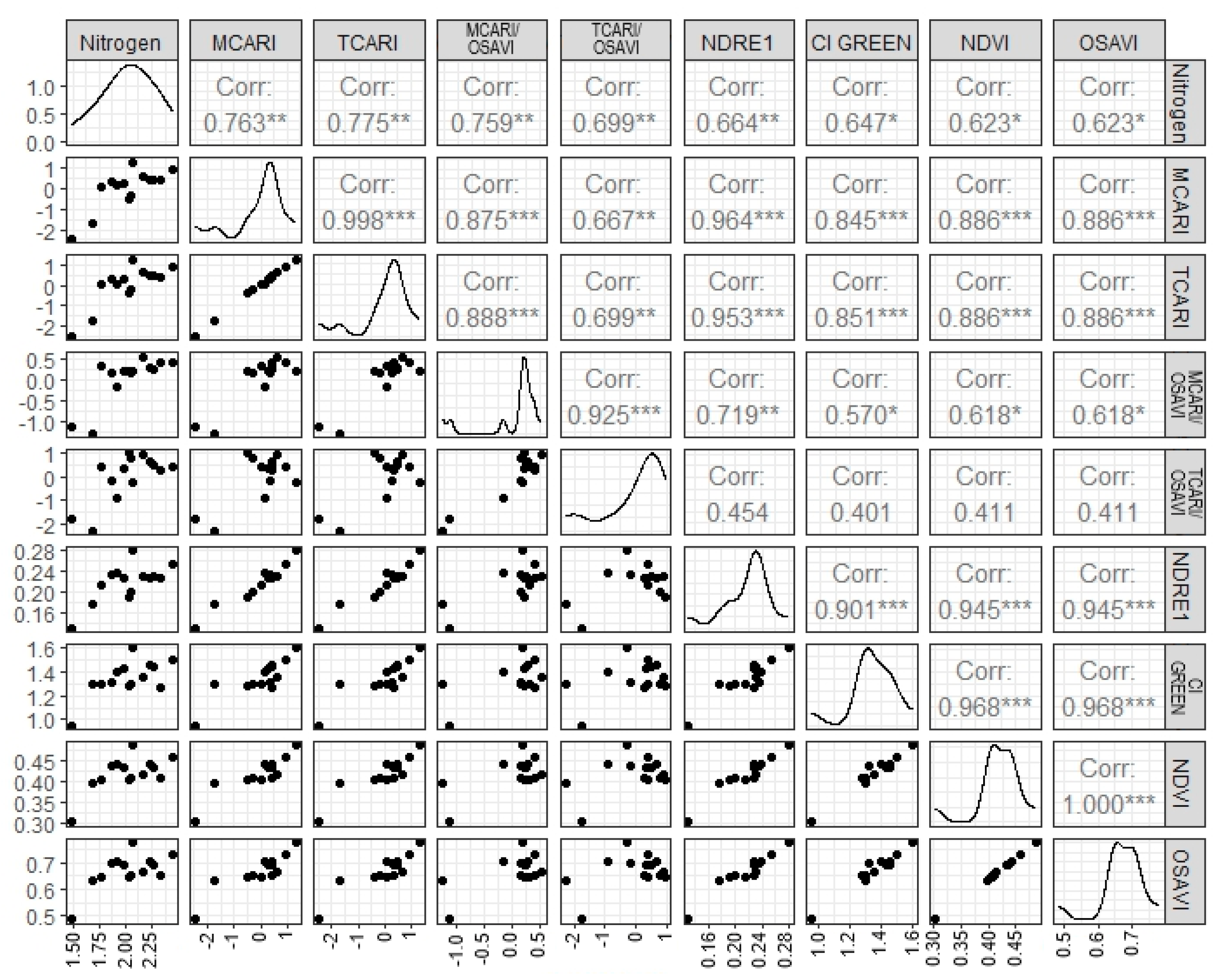
The nitrogen values obtained in the laboratory range from 1.49% to 2.45%, with a mean of 2.00% and a median of 1.49%. Figure 2 shows the relationship between the vegetation indices and nitrogen, evaluated through Pearson correlation (Figure 3). It is observed that the TCARI, MCARI, TCARI/OSAVI, and MCARI/OSAVI indices show a correlation equal to or greater than 0.7 with the nitrogen content.
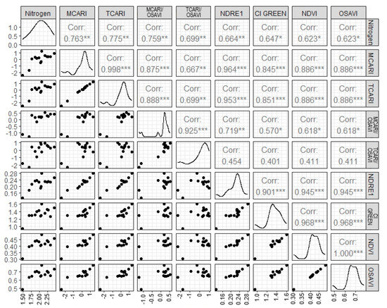
Figure 3.
Pearson correlation matrix with different vegetation indices. Significance * 90, ** 95, and *** 99. Corr, correlation; MCARI, Modified Chlorophyll Absorption in Reflectance Index; TCARI, Transformed Chlorophyll Absorption in Reflectance Index; OSAVI, Optimized Soil Adjusted Vegetation Index; NDRE 1, Normalized difference red-edge 1; CI GREEN, Chlorophyll index green; NDVI, Normalize difference vegetation index.
3.2. Nitrogen Estimation with Artificial Intelligence Algorithms
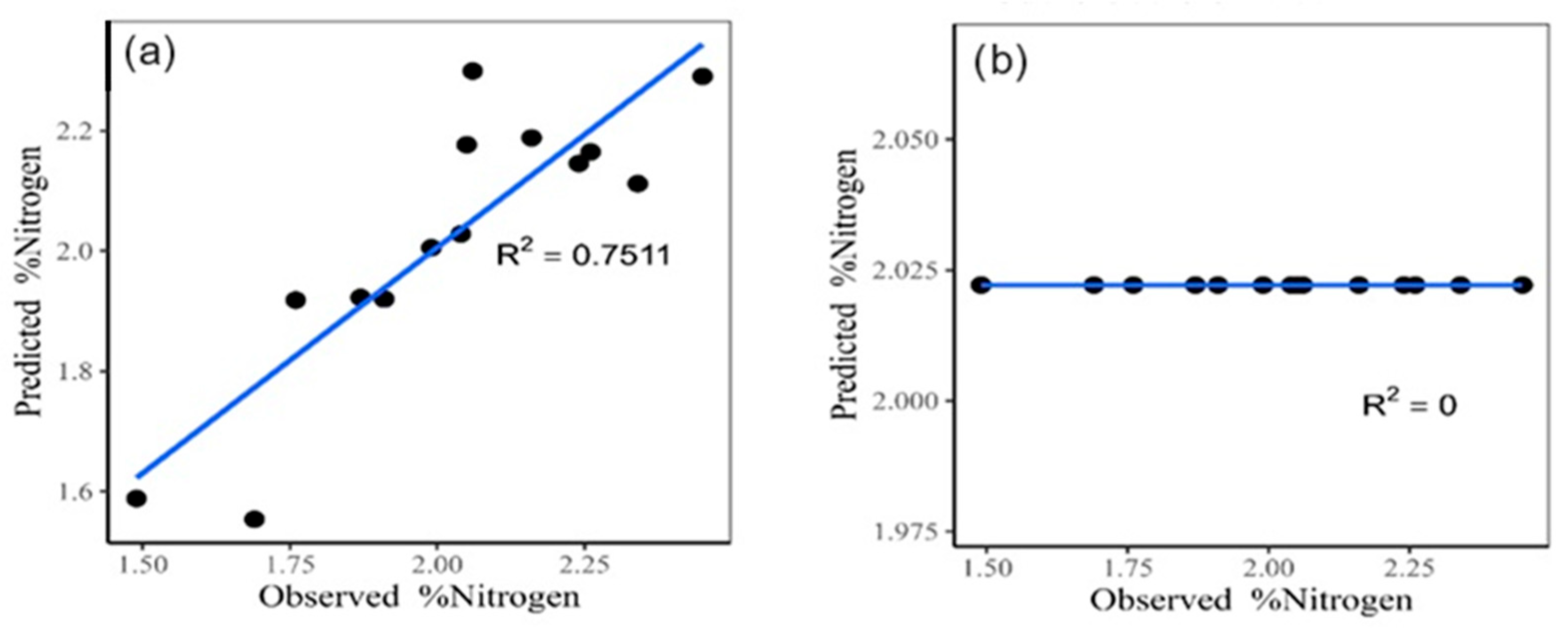
The classic multiple linear regression model (Figure 4a), which was performed in R software (https://www.r-project.org/, accessed on 6 September 2022) incorporating the four most important variables according to Pearson’s correlation, has an explained variance of 75.11%, a mean square error (MSE) of 0.0162, and a mean square error (MSE) of 0.1271. On the other hand, when using the random forest model (Figure 4b), a coefficient of determination (R2) of zero, an MSE of 0.0649, and an RMSE of 0.2548 are observed.
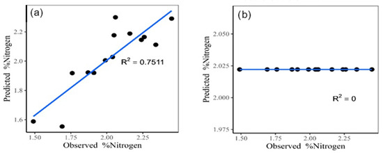
Figure 4.
Classic multiple linear regression model for nitrogen estimate (a). Random forest for nitrogen estimate (b).
Using gradient boosting (Figure 5a), 78.77% of the variance is explained, with an MSE of 0.0138 and an RMSE of 0.1174. In this model, it is observed that the TCARI index has a lower relevance, while the MCARI/OSAVI stands out as the most influential for the estimation of the nitrogen content (Figure 5b).
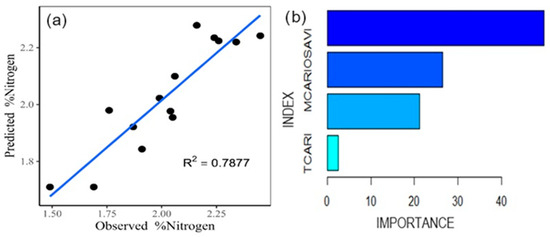
Figure 5.
Gradient boosting model for nitrogen estimation (a). Relative influence of the indices (b).
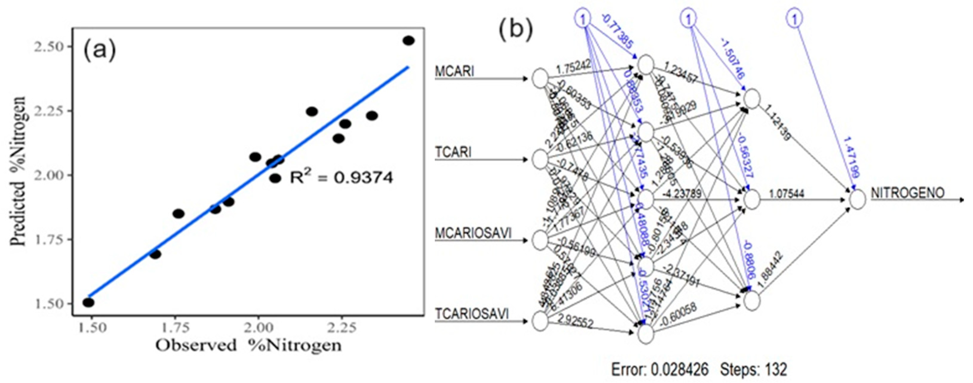
Artificial neural networks (Figure 6a), with a hidden layer arrangement of 5, 3 (Figure 6b), shows a variance of 93.74%, MSE of 0.0041, and RMSE of 0.0637.
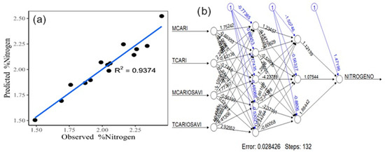
Figure 6.
Scatterplot of the neural network model for nitrogen estimation (a). Conceptualization of artificial neural networks with the selected vegetation indices (b).
The above demonstrates that the best model for estimating the foliar nitrogen content is artificial neural networks, statistically presenting the most significant values related to the laboratory-calculated nitrogen content.
4. Discussion
The results of the linear regression model are similar to those reported by López-Calderón et al., 2023 [52], where they estimate the nitrogen content in forage maize with different spectral indices and Sentinel-2 images, highlighting, as the optimal model, the set of MCARI/OSAVI, MCARI/OSAVI RE, TCARI/OSAVI, and TCARI/OSAVI RE indices, with an R2 coefficient of 0.56.
Xiong et al. (2019) [53], in their study of the nitrogen nutrition index for Brassica campestris ssp. chinensis L., concluded that plants with excess nitrogen reflect less visible light than those plants deficient in nitrogen, and also defined that the random forest method provides a better prediction during the seedling and harvest stages; on the other hand, Abdel-Rahman et al. (2013) [49] used random forest and identified the most relevant ranges of the visible spectrum for estimating the nitrogen content, which encompasses the visible light (400–700 nm), the red edge (670–780 nm), and the mid-infrared (1300–2500 nm) of the electromagnetic spectrum in sugarcane. These results are complemented by those obtained by Ramalho-de-Oliveira et al. (2017) [54], where they highlight the wavelength ranges between 400 and 900 nm for nitrogen estimation, and observed a lower reflectance intensity in the 400 to 700 nm range and higher reflectance between 740 and 900 nm. These results differ slightly from those mentioned above, since the spectral indices selected for the best estimation of the nitrogen content are in a narrower range, between 705 and 750 nm of the electromagnetic spectrum. It is important to note that the fig tree is native to the Mediterranean [55], while the experiment was conducted in northern Mexico. On the other hand, eucalyptus [53] is native to Australia and Tasmania, and the research was carried out in north–central Brazil. These differences may be related to the specific characteristics of the genotypes and agro-climatological conditions of the different regions.
In the study conducted in 2024 by Yiping Peng et al., [56] different machine-learning methodologies were used to estimate the nitrogen content of rice leaves, in which they concluded that Pearson’s correlation coefficient, in conjunction with extreme gradient boosting, significantly improves the accuracy of estimating the nitrogen content of rice compared to the independent screening approach; however, the vegetation indices used in that work are different from those used in the present study.
Regarding the artificial neural networks, the results obtained using the four indices, MCARI, MCARI/OSAVI, TCARI, and TCARI/OSAVI, with an explained variance of 93% present a great similarity with the work presented by Martínez-Sifuentes et al. (2024) [57], where they use 15 vegetation indices to estimate the nitrogen content in forage maize, which explains 83% of the variance; however, the NDREmax and TCARImax indices explain 79% of the variance, which indicates that, by relating few indices, it is possible to have solid results.
The vegetation indices MCARI, TCARI, MCARI/OSAVI, and TCARI/OSAVI coincide with the results of Wang et al. (2016) [58], where the MCARI and MCARI/OSAVI indices, calculated using wavelengths of 750 and 705 nm, present a greater precision in the estimation of the nitrogen content in temperate forests. On the other hand, De Sousa et al. (2020) [59] determined that the best index for estimating the nitrogen content in the vegetative phase of the chili crop was GNDVI. Similarly, they highlight that, in the early fruit growth phase, the best index is GVI. These discrepancies highlight the importance of considering the specific characteristics of each crop, as well as the different phenological stages, when selecting appropriate vegetation indices for estimating variables such as nitrogen content.
The difference between the optimal vegetation indices for different crops, such as chili and fig, is related to morphological variations; for example, chili, being a vegetable, has less leaf area compared to a tree such as fig, which, even if it is pruned, will have a larger leaf area [60]. This suggests that there is a relationship between these vegetation indices and nitrogen content, indicating the possibility of using artificial intelligence algorithms to determine this association with a greater precision.
5. Conclusions
Currently, there are research studies for various crops and spectral indices that aim to establish a close relationship between these indices and the nitrogen content under field conditions or extensive management. However, there is little or no bibliography on the fig crop and its relationship with spectral indices, so, with the help of artificial intelligence algorithms, algorithms that improve or discard certain relationships between all these variables are proposed.
In the present study, the most important vegetation indices for the estimation of nitrogen in the fig crop were TCARI, MCARI, TCARI/OSAVI, and MCARI/OSAVI, all of which were in the range of 705 nm to 750 nm. When related to the classical models of multiple linear regression, random forest, gradient boosting, and artificial neural networks, it was shown that the best methodology for estimating the content of this macronutrient was artificial neural networks, a model that explains 93% of the variance between these indices and the nitrogen content in fig.
The estimation of plant nitrogen using geospatial techniques has gained great relevance in recent years due to the practicality of these techniques, which optimize the detection of deficiencies and lead to savings in time and money, allowing timely decision-making for sustainable crop management.
Author Contributions
Conceptualization, A.R.M.-S., K.J.M.-M. and S.Y.M.-G.; methodology, A.R.M.-S. and R.T.-C.; software, A.R.M.-S., K.J.M.-M. and A.R.-G.; formal analysis, A.R.M.-S. and K.J.M.-M.; resources, R.T.-C., A.R.-G., P.P.-R. and P.Y.-C.; writing—original draft preparation, K.J.M.-M.; writing—review and editing, A.R.M.-S., S.Y.M.-G. and A.R.-G.; project administration, A.R.M.-S. and S.Y.M.-G. All authors have read and agreed to the published version of the manuscript.
Funding
This research received no external funding.
Data Availability Statement
The datasets presented in this article are not readily available because the data are part of a ongoing study. Requests to access the datasets should be directed to martinez.aldo@inifap.gob.mx.
Conflicts of Interest
The authors declare no conflicts of interest.
References
- Schmidt-Durán, A.; Chacón-Cerdas, R. Desarrollo del ciclo de vida y comparación de la fertilidad de Estigmene albida aislada del cultivo del higo (Ficus carica), bajo condiciones controladas de laboratorio. Tecnol. Marcha 2023, 36, 117–129. [Google Scholar] [CrossRef]
- Secretaría de Agricultura y Desarrollo Rural. Qué Hay Detrás de la Producción de Higo. 2023. Available online: https://www.gob.mx/agricultura/articulos/que-hay-detras-de-la-produccion-de-higo?idiom=es#:~:text=En%202022%2C%20el%20pa%C3%ADs%20cosech%C3%B3,Baja%20California%20Sur%20y%20Michoac%C3%A1n (accessed on 18 June 2024).
- Martínez-Macias, K.J.; Márquez-Guerrero, S.Y.; Martínez-Sifuentes, A.R.; Segura-Castruita, M.A. Habitat Suitability of Fig (Ficus carica L.) in Mexico under Current and Future Climates. Agriculture 2022, 12, 1816. [Google Scholar] [CrossRef]
- Algas Pacific. Bioestimulación y Nutrición Específica en el Cultivo de Higo. 2023. Available online: https://algaspacific.com/2022/03/23/bioestimulacion-y-nutricion-especifica-en-el-cultivo-de-higo/ (accessed on 18 June 2024).
- Córdoba-Domínguez, A.; Delgado-García, M.; Hernández-Castillo, F.D.; González, V. Microorganismos fijadores de nitrógeno: Esenciales para la vida. CienAcie 2013, 9, 29–32. [Google Scholar]
- Sosa-Rodrigues, B.A.; García-Vivas, Y.S. Eficiencia de uso del nitrógeno en maíz fertilizado de forma orgánica y mineral. Agron. Mesoam. 2018, 29, 207–219. [Google Scholar] [CrossRef]
- Zelia-Silva, A.; Wamser-Nowaki, F.; Hiyoshi, R.; Filho, C.; Bernardes, A.; Mendoza-Cortez, J.W. Síntomas de deficiencia de macronutrientes en pimiento (Capsicum annuum L.). Agrociencia 2017, 21, 31–43. [Google Scholar] [CrossRef]
- Fernández-Pavía, Y.L.; García-Cue, J.L.; Fernández-Pavía, S.P.; Muratalla Lúa, A. Deficiencias nutrimentales inducidas en higuera cv. Neza en condiciones hidropónicas. Rev. Mex. Cienc. Agríc. 2020, 11, 581–592. [Google Scholar] [CrossRef]
- NASA Arset. Fundamentos de la Teledetección (Persepción Remota). 2023. Available online: https://appliedsciences.nasa.gov/sites/default/files/2023-03/Fundamentals_of_RS_Span.pdf (accessed on 12 October 2023).
- Copernicus. Fundamentos de Teledetección Aplicada. El Programa Copernicus Aplicado a la Producción y Gestión de la Información Geoespacial. Proyecto Cofinanciado por la Comisión Europea Mediante Acuerdo 2018/SI2.810140/04. 2018. Available online: https://www.ign.es/web/resources/docs/IGNCnig/actividades/OBS/Programa_Marco_Copernicus_User_Uptake/2_Fundamentos_teledeteccion_aplicada.pdf (accessed on 27 June 2024).
- Salva, M.; Campo, S.; Romo, A.; Salvador, F.; Cortés, A.; Padrón, P.A.; Boratyński, A. Análisis de índices de vegetación de los sabinares de el hierro con imágenes de satélite de muy alta resolución. In La Naturaleza Atlántica: Hábitats, Patrimonio y Vulnerabilidad. II Congreso Iberoamericano y XII Congreso Español de Biogeografía; De la Llama Editorial: San Pedro, Spain, 2022; pp. 167–173. ISBN 978-84-124632-9-3. Available online: http://hdl.handle.net/10261/347687 (accessed on 27 June 2024).
- Buzzi, M.A.; Rueter, B.L.; Ghermandi, L. Múltiples índices espectrales para predecir la variabilidad de atributos estructurales y funcionales en zonas áridas. Ecol. Austral. 2017, 27, 55–62. Available online: http://hdl.handle.net/11336/30772 (accessed on 27 June 2024). [CrossRef]
- Bonnaire-Rivera, L.; Montoya-Bonilla, B.; Obando-Vidal, F. Procesamiento de imágenes multiespectrales captadas con drones para evaluar el índice de vegetación de diferencia normalizada en plantaciones de café variedad Castillo. Cienc. Tecnol. Agropecu. 2021, 22, 1–16. [Google Scholar] [CrossRef]
- Corrales-González, M.; Rada, F.; Jaimez, R. Efecto del nitrógeno en los parámetros fotosintéticos y de producción del cultivo de la gerbera (Gerbera jamesonii H. Bolus ex Hook. f.). Acta Agron. 2016, 65, 255–260. [Google Scholar] [CrossRef]
- Haboudane, D.; Miller, J.R.; Tremblay, N.; Zarco-Tejada, P.J.; Dextraze, L. Integrated narrow-band vegetation indices for prediction of crop chlorophyll content for application to precision agriculture. Remote Sens. Environ. 2002, 81, 416–426. [Google Scholar] [CrossRef]
- Innovatione AgroFood Design. Índices de Vegetación en Agricultura de Precisión. 2020. Available online: https://innovatione.eu/2020/04/20/indices-vegetacion-agricultura-precision/ (accessed on 5 May 2022).
- Alvarado-Salazar, R.; Llerena-Izquierdo, J. Revisión de la literatura sobre el uso de Inteligencia Artificial enfocada a la atención de la discapacidad visual. InGenio J. 2022, 5, 10–21. [Google Scholar] [CrossRef]
- FCCyT (Foro Constitutivo Científico y Tecnológico). Inteligencia Artificial. INCyTU 2018, 12, 1–6. [Google Scholar]
- Mena, A.; de Oliveira-Cardoso, N.; Xavier, C.E.; de Lina-Argimon, I. Técnicas de Machine Learning utilizadas en estudios psicológicos con adolescentes: Una revisión sistemática. Rev. Psicol. Educ. 2022, 20, 23–37. [Google Scholar] [CrossRef]
- Ordóñez-Erazo, H.A.; Ordoñez-Quintero, C.C.; Bucheli-Guerrero, V.A. Un modelo basado gradient boosting regressor para predecir tendencias de razón de residencia en relación a la edad de los habitantes de la calle en Colombia. Rev. Ibérica Sist. Tecnol. Informação 2023, 11, 145–157. [Google Scholar] [CrossRef]
- Das, B.; Rathore, P.; Roy, D.; Chakraborty, D.; Jatav, R.S.; Sethi, D.; Kumar, P. 2022. Comparison of bagging, boosting and stacking algorithms for surface soil moisture mapping using optical-thermal-microwave remote sensing synergies. Catena 2022, 217, 106485. [Google Scholar] [CrossRef]
- Odegua, R. An empirical study of ensemble techniques (bagging, boosting and stacking). In Proceedings of the Conference on Deep Learning IndabaXAt, Lagos, Nigeria, 9–10 May 2019. [Google Scholar] [CrossRef]
- Graczyk, M.; Lasota, T.; Trawiński, B.; Trawiński, K. Comparison of bagging, boosting and stacking ensembles applied to real estate appraisal. In Proceedings of the Intelligent Information and Database Systems: Second International Conference, ACIIDS, Hue City, Vietnam, 24–26 March 2010. [Google Scholar]
- Montiel-González, R.; Bolaños-González, M.A.; Macedo-Cruz, A.; Rodríguez-González, A.; López-Pérez, A. Clasificación de uso del suelo y vegetación con redes neuronales convolucionales. Rev. Mex. Cienc. For. 2022, 13, 97–119. [Google Scholar] [CrossRef]
- Estrada-Zúñiga, A.C.; Cárdenas-Rodríguez, J.; Bejar-Saya, J.V.; Ñaupari-Vásquez, J. Estimación de la biomasa de una comunidad vegetal altoandina utilizando imágenes multiespectrales adquiridas con sensores remotos UAV y modelos de Regresión Lineal Múltiple, Máquina de Vectores Soporte y Bosques Aleatorios. Sci. Agropecu. 2022, 13, 301–310. [Google Scholar] [CrossRef]
- Guerrero-Meza, J.R.; Villanueva-Mejía, J.A.; Renteros-Parra, B.E.; Castañeda-Valdivieso, R.E. Detección de Nutrientes del Suelo y Planta, y Pestes en Campos de Cultivo de Banano Orgánico con Machine Learning. Universidad de Piura. 2021. Available online: https://hdl.handle.net/11042/5204 (accessed on 27 June 2024).
- De Lara, A.; Mieno, T.; Luck, J.D.; Puntel, L. Predicting site-specific economic optimal nitrogen rate using machine learning methods and on-farm precision experimentation. Precis. Agric. 2023, 24, 1792–1812. [Google Scholar] [CrossRef]
- INEGI [Instituto Nacional de Estadística y Geografía]. Compendio de Información Geográfica Municipal 2010; Gómez Palacio, Durango. 2010. 10p. Available online: https://www.inegi.org.mx/contenidos/app/mexicocifras/datos_geograficos/10/10007.pdf (accessed on 27 June 2024).
- INEGI [Instituto Nacional de Estadística y Geografía]. Aspectos Geográficos Durango. 2021. 45p. Available online: https://www.inegi.org.mx/contenidos/app/areasgeograficas/resumen/resumen_10.pdf (accessed on 27 June 2024).
- Lichtenthaler, H.K. Chlorophylls and Carotenoids: Pigments of Photosynthetic Biomembranes. Methods Enzymol. 1987, 148, 350–382. [Google Scholar] [CrossRef]
- Salvador-Castillo, J.M.; Bolaños-González, M.A.; Palacios-Vélez, E.; Palacios-Sánchez, L.A.; López-Pérez, A.; Muñoz-Pérez, J.M. Estimación de la fracción de cobertura vegetal y contenido de nitrógeno del dosel en maíz mediante sensores remotos. Terra Latinoam. 2021, 39, e899. [Google Scholar] [CrossRef]
- Feng, L.; Zhang, Z.; Ma, Y.; Du, Q.; Williams, P.; Drewry, J.; Luck, B. Alfalfa yield prediction using UAV-based hyperspectral imagery and ensemble learning. Remote Sens. 2020, 12, 2028. [Google Scholar] [CrossRef]
- ESRI (Environmental Systems Research Institute). ArcGIS Desktop: Redlands, CA, USA, 2019. Release 10.8. Available online: https://www.esri.com/es-es/arcgis/about-arcgis/overview (accessed on 27 June 2024).
- Jiménez-Jiménez, S.I.; Marcial-Pablo, M.D.J.; Ojeda-Bustamante, W.; Sifuentes-Ibarra, E.; Inzunza-Ibarra, M.A.; Sánchez-Cohen, I. VICAL: Global calculator to estimate vegetation indices for agricultural areas with landsat and sentinel-2 data. Agronomy 2022, 12, 1518. [Google Scholar] [CrossRef]
- Gitelson, A.A.; Gritz, Y.; Merzlyak, M.N. Relationships between leaf chlorophyll content and spectral reflectance and algorithms for non-destructive chlorophyll assessment in higher plant leaves. J. Plant Physiol. 2003, 160, 271–282. [Google Scholar] [CrossRef]
- Wu, C.; Niu, Z.; Tang, Q.; Huang, W. Estimating chlorophyll content from hyperspectral vegetation indices: Modeling and validation. Agric. For. Meteorol. 2008, 148, 1230–1241. [Google Scholar] [CrossRef]
- Gitelson, A.; Merzlyak, M.N. Quantitative estimation of chlorophylla using reflectance spectra: Experiments with autumn chestnut and mapleleaves. J. Photochem. Photobiol. B Biol. 1994, 22, 247–252. [Google Scholar] [CrossRef]
- Rouse, J.W.; Haas, R.H.; Schell, J.A.; Deering, D.W. Monitoring vegetation systems in the Great Plains with ERTS, third ERTS symposium. NASA Spec. Publ. 1974, 1, 309–351. [Google Scholar]
- Rondeaux, G.; Steven, M.; Baret, F. Optimization of soil-adjusted vegetation indices. Remote Sens. Environ. 1996, 55, 95–107. [Google Scholar] [CrossRef]
- Basoalgin-Olabe, X. Introducción a la computación neuronal. In Redes Neuronales Artificiales y sus Aplicaciones; Escuela Superior de Ingeniería de Bilbao: Bilbao, Spain, 2006; pp. 1–12. [Google Scholar]
- Perdigón-Llanes, R.; González-Benítez, N. Redes neuronales artificiales en el pronóstico de la producción de leche bovina. Rev. Colomb. Comput. 2022, 23, 20–33. [Google Scholar] [CrossRef]
- Ríos-Ríos, B. Diagnóstico del dengue utilizando redes neuronales artificiales. Cienc. Lat. Rev. Científica Multidiscip. 2022, 6, 5636–5651. [Google Scholar] [CrossRef]
- Saldaña, C.A.; Kuonquí-Gaínza, F.I.; Malave-Vivar, C.A.; Tumbaco-Reyes, A.R.; Pasmay-Bohórquez, P.I. Simulación y comparación de controladores PID, Liapunov y redes neuronales artificiales: Abordando el rechazo de perturbaciones en sistemas no lineales a través de modelado computacional. Cienc. Lat. Rev. Científica Multidiscip. 2023, 7, 3849–3865. [Google Scholar] [CrossRef]
- Mercado-Polo, D.; Pedraza-Caballero, L.; Martínez-Gómez, E. Comparación de Redes Neuronales aplicadas a la predicción de Series de Tiempo. Prospectiva 2015, 13, 88–95. [Google Scholar] [CrossRef][Green Version]
- Espinosa-Zúñiga, J.J. Aplicación de algoritmos Random Forest y XGBoost en una base de solicitudes de tarjetas de crédito. Ing. Investig. Tecnol. 2020, 21, 1–16. [Google Scholar] [CrossRef]
- Cimarra-Muñoz, D. Experimentos de Predicción con Gradient Boosting y Random Forest. Bachelor’s Thesis, Universidad Politécnica de Madrid, Madrid, Spain, 2018. [Google Scholar]
- Cánovas-García, F.; Alonso-Sarría, F.; Gomariz-Castillo, F. Modificación del algoritmo Random Forest para su empleo en clasificación de imágenes de teledetección. In Proceedings of the Aplicaciones de las Tecnologías de la Información Geográfica (TIG) para el Desarrollo Económico Sostenible, XVII Congreso Nacional de Tecnologías de Información Geográfica, Málaga, Spain, 29 June–1 July 2016; pp. 359–368. [Google Scholar]
- Blanco-Murillo, D.M.; García-Domínguez, A.; Galván-Tejada, C.E.; Celaya-Padilla, J.M. Comparación del nivel de precisión de los clasificadores Support Vector Machines, k Nearest Neighbors, Random Forests, Extra Trees y Gradient Boosting en el reconocimiento de actividades infantiles utilizando sonido ambiental. Res. Comput. Sci. 2018, 147, 281–290. [Google Scholar] [CrossRef]
- Abdel-Rahman, E.M.; Ahmed, F.B.; Ismail, R. Random forest regression and spectral band selection for estimating sugarcane leaf nitrogen concentration using EO-1 Hyperion hyperspectral data. Int. J. Remote Sens. 2013, 34, 712–728. [Google Scholar] [CrossRef]
- Prado Osco, L.; Marquez, A.P.; Roberto, D.; Akemi, É.; Nobuhiro, N.; Takashi, E.; Estrabis, N.; de Souza, M.; Junior, J.M.; Gonçalves, W.N. Predicting Canopy Nitrogen Content in Citrus-Trees Using Random Forest Algorithm Associated to Spectral Vegetation Indices from UAV-Imagery. Remote Sens. 2019, 11, 2925. [Google Scholar] [CrossRef]
- Zhang, M.; Tsoulakos, N.; Kujala, P.; Hirdaris, S. A deep learning method for the prediction of ship fuel consumption in real operational conditions. Eng. Appl. Artif. Intell. 2024, 130, 107425. [Google Scholar] [CrossRef]
- López-Calderón, M.; Estrada-Ávalos, J.; Martínez-Sifuentes, A.R.; Trucíos-Caciano, R.; Miguel-Valle, E. Total Nitrogen in forage corn (Zea mays L.) estimated by satelliteSentinel-2 spectral índices. Terra Latinoam. 2023, 41, e1628. [Google Scholar] [CrossRef]
- Xiong, X.; Zhang, J.; Guo, D.; Chang, L.; Huang, D. Non-Invasive Sensing of Nitrogen in Plant Using Digital Images and Machine Learning for Brassica Campestris ssp. Chinensis L. Sensors 2019, 19, 2448. [Google Scholar] [CrossRef]
- Ramalho-de-Oliveira, L.F.; Ramalco-de-Oliveira, M.L.; Sergio-Gomes, F.; Campos-Santana, R. Estimating foliar nitrogen in Eucalyptus using vegetation indexes. Sci. Agric. 2017, 74, 142–147. [Google Scholar] [CrossRef]
- Solís-Pino, A.F.; Revelo-Luna, D.A.; Campo-Ceballos, D.A.; Gaviria-López, C.A. Correlación del contenido de clorofila foliar de la especie Coffea arabica con índices espectrales en imágenes. Biotecnol. Sect. Agropecu. Agroind. 2021, 19, 57–68. [Google Scholar] [CrossRef]
- Peng, Y.; Zhong, W.; Peng, Z.; Tu, Y.; Xu, Y.; Li, Z.; Liang, J.; Huang, J.; Liu, X.; Fu, Y. Enhanced Estimation of Rice Leaf Nitrogen Content via the Integration of Hybrid Preferred Features and Deep Learning Methodologies. Agronomy 2024, 14, 1248. [Google Scholar] [CrossRef]
- Martínez-Sifuentes, A.R.; Trucíos-Caciano, R.; López-Hernández, N.A.; Miguel-Valle, E.; Estrada-Ávalos, J. Spectral Index-Based Estimation of Total Nitrogen in Forage Maize: A Comparative Analysis of Machine Learning Algorithms. Nitrogen 2024, 5, 468–482. [Google Scholar] [CrossRef]
- Wang, Z.; Wang, T.; Darvishzadeh, R.; Skidmore, A.K.; Jones, S.; Suarez, L.; Woodgate, W.; Heiden, U.; Heurich, M.; Hearne, J. Vegetation indices for mapping canopy foliar nitrogen in a mixed temperate forest. Remote Sens. 2016, 8, 491. [Google Scholar] [CrossRef]
- De-Souza, R.; Peña-Fleitas, M.T.; Thompson, R.B.; Gallardo, M.; Padilla, F.M. Assessing performance of vegetation indices to estimate nitrogen nutrition index in pepper. Remote Sens. 2020, 12, 763. [Google Scholar] [CrossRef]
- Márquez-Guerrero, S.Y.; Figueroa-Viramonetes, U.; Cueto-Wong, J.A.; Arreola-Ávila, J.G.; Zegbe-Domínguez, J.A.; Trejo-Calzada, R. Variación estacional de la concentración foliar de nutrimentos en huertas de higuera bajo sistemas de producción intensiva. Rev. Mex. Cienc. Agríc. 2019, 10, 525–537. [Google Scholar] [CrossRef]
Disclaimer/Publisher’s Note: The statements, opinions and data contained in all publications are solely those of the individual author(s) and contributor(s) and not of MDPI and/or the editor(s). MDPI and/or the editor(s) disclaim responsibility for any injury to people or property resulting from any ideas, methods, instructions or products referred to in the content. |
© 2024 by the authors. Licensee MDPI, Basel, Switzerland. This article is an open access article distributed under the terms and conditions of the Creative Commons Attribution (CC BY) license (https://creativecommons.org/licenses/by/4.0/).

