Proceeding Paper

Dynamical Downscaling of Future Climate Change Scenarios in Urban Heat Island and Its Neighborhood in a Brazilian Subtropical Area †

by
Marcos Vinicius Bueno de Morais
1,*,
Viviana Vanesa Urbina Guerrero
2,
Leila Droprinchinski Martins
3 and
Jorge Alberto Martins
4
1
Post-Graduate Program in Environmental Engineering, Federal Technology University—Paraná, Londrina 86036-370, Brazil
2
Post-Graduate Program in Electrical Engineering, Federal Technology University—Paraná, Cornélio Procópio 86300-000, Brazil
3
Chemistry Department, Federal Technology University—Paraná, Londrina 86036-370, Brazil
4
Physics Department, Federal Technology University—Paraná, Londrina 86036-370, Brazil
*
Author to whom correspondence should be addressed.
Presented at the 2nd International Electronic Conference on Atmospheric Sciences, 16–31 July 2017; Available online: http://sciforum.net/conference/ecas2017.
Proceedings 2017, 1(5), 106; https://doi.org/10.3390/ecas2017-04130
Published: 17 July 2017

Abstract

:
According to IPCC reports, a greater frequency, intensity and duration of heat waves in urban areas are expected. This is related to the dynamical evolution of the cities, due the changes of the natural surface modifies the roughness pattern reduce the wind intensity, modify the available humidity in the soil and the radiative properties. These topics characterize the formation of the urban heat island (UHI). A dynamical downscaling of A2 and B1 future scenarios was made for Londrina, a medium-size city of Southern Brazil, using Weather Research Forecasting model, to investigate the impact of this projections on the UHI formation and intensity, as well for rural area, which consistent an important agricultural landscape. For this, an evaluation of the model and the scenarios were done to investigate the current trends. The results shows a tendency of following the worst proposed scenarios (A2), and a drier rural area for the sustainable projection, which has directly influence on the urban heat island intensity and formation, and in the agriculture of the region.

1. Introduction

The study of the climate in urban areas is one of the most priority places when the central topic is the climate changes impacts, because today more than 50% of world population lives in urban regions. According to the last two IPCC reports [1,2], there are a prediction of more frequent occurrence of heat waves in urban areas, with higher intensity and duration [3].
Previous studies have showed that urban areas are vulnerable to extreme events and climate changes. For example in 2003, about 35 thousand people died because of a heat wave in the west Europe [4]. Numerical studies employing the A1B scenario from IPCC [5] shows that the Frankfurt city, in Germany, could present more days (about 32) with maximum temperature above 25 °C for the period between 2021 and 2050, compared to 1971 to 2000 [6]. For Brussels and Paris, using the same A1B scenario, the projection are that the temperature will increase about 1.6 °C and 1.8 °C, respectively in 2050-year [7]. This study also found a pattern in the changes of the temperatures between the city and rural areas, for the nocturnal period in winter (with increase of 0.2 °C) and diurnal in summer (with decrease in −0.1 °C). In this case, the decrease in summer was resulted from a drier rural area.
The dynamic evolution of cities has also an important role in the impact on future climate scenarios. The urban planning it can help to minimize the climate change effects, otherwise may increase the negative effects. Simulations varying the growth of urban area in three different ways (current status, compact growth and spread growth) to the Metropolitan Area of Tokyo for 2070 shows that the humid bulb temperature can increase of 4 °C higher during the daytime depending on the urban expansion mode [8]. In a similar way, using same scenarios, for Paris in 2100, numerical simulations shows that the variation of the heat waves risk does not depends only of the dynamic expansion, but also of the population exposure, because in the situations that the urban area are more compact, the population is more vulnerable to feel the effects of extreme temperatures [9].
The increase of temperature in the future can reduce the thermal comfort mainly in urban areas. For example, excess hospital admissions can be by dehydration, heat stroke, and heat exhaustion, among people with underlying medical condition [10]. Moreover, the interventions in the natural surface by the urbanization causes changes on roughness, reducing wind speed, moisture availability in the soil and radiative properties [11]. These changes affect the local microclimate and can contribute to Urban Heat Island (UHI; [12]). This is a transient feature of urban areas where the air temperature near the surface of the city is higher than the temperature of the surrounding rural areas. The study of UHI is very difficult, because the role of rural areas in determining the magnitude and the structure of UHI cannot be understood [13]. Its intensity may vary due to the size of the city, wind speed, cloud cover [14], and to the geographical location of the urban area. In addition, its intensity is strongly related to both the morphology of cities, and for the construction material properties. In mid-latitudes, the UHI is more intense during the night, while in tropical latitudes, its development takes place during the day [12,15,16]. The study of UHI is of fundamental importance because they can aggravate the effects of extreme temperatures caused by heat waves [17] or other extreme events.
Since the importance of urban areas in the microclimate of a region, to study of the thermal and dynamic properties of a city it is important for a great number of applications. The resulting stress of UHI can become a public health problem [18] as well as the dispersion of pollutants due to local features [19] and synoptic conditions [20,21]. Furthermore, civil engineers and architects need detailed knowledge of the wind in urban areas, to determine the length of the structure and the energy required for new buildings [22,23]. So with the computational development, numerical weather forecast models have become an important tool in the study of urban boundary layer.
There are several studies for Brazil discussing climate change scenarios [24,25,26]. However, considering the Brazilian dimension and large differences in climatic conditions, local effects on the climate cannot be completely addressed. Moreover, are rare the studies of climate change scenarios using high resolution simulation as proposed in this work.
One city that present UHI is Londrina, which is a medium sized-city has witnessed major urban and population growth in recent decades, with more than 500 thousands inhabitants [27], and is located in a subtropical region. Daytime UHI intensity in Londrina is about 2 °C for a summer period [28]. Based on this information, the main objective of this work is to investigate the physics in the UHI formation and intensity on the most extremes future climate change scenarios from the IPCC, A2 and B1.

2. Experiments

2.1. Future Scenarios

The SRES (Special Report on Emission Scenarios) describes a series of future scenarios, developed by IPCC and based in different factors that can influence the emissions, as demography, technology and economy [5]. These scenarios uses a variety of possibilities based on global development, which are associated to CO2 sources and sinks, and other greenhouses gases, from alternative sources of energy to soil land use changes. The group of the scenarios includes the more relevants greenhouse gas effect from anthropogenic emission, besides other compounds, like sulfur dioxide (SO2), carbon monoxide (CO), nitrogen oxides (NOx) and non-methane hydrocarbons (NMHC). Given that future emissions have many uncertainties, the analysis of these scenarios is an important task to evaluate the variability of the results.
SRES presents 40 different scenarios developed by six modeling teams separated into six groups of four families, which is one group into A2, B1, B2, and three groups within the family A1. The latter is based on the alternative development of energy technologies: A1FI (intensive fossil fuel), A1B (balanced), and A1T (predominantly non-fossil fuel). Within each family and group of scenarios, some assumptions are done about global population, gross world product, and the final energy “harmonized”. In addition, the total annual global emission of CO2 based on all sources (energy, industry and change in land use) for the period 1990–2100 [in gigatonnes of carbon (GTC/year)] are considered for the four families (A1, A2, B1, and B2) and six scenario groups.
In this work, we considered the SRES scenarios A2 and B1 from IPCC, because A2 and B1 describe a pessimist and optimist scenarios, respectively. The A2 describes a very heterogeneous world, with continuous increasing of the population, and the per capita economic growth and technological change are more fragmented and slower than other storylines. On the other hand, the B1 storyline and scenario family describes a convergent world with the same global population, where the emphasis is on global solutions to economic, social and environmental sustainability, including improved equity, but without additional climate initiatives. The illustration of two scenarios are shown in Figure 1, as well the emission band (colored), which denotes the range of scenarios harmonized and not harmonized within family.

2.2. Numerical Modeling and Configuration

For this study, it was used the version 3.6.1 of the atmospheric model WRF (Weather Research and Forecast, [29]). This model represents the last generation of numerical weather prediction, that works even for operational as research use. This model is in constant development, as a partnership of several agencies, like National Center for Atmospheric Research (NCAR), National Oceanic and Atmospheric Administration (NOAA), National Center for Environmental Prediction (NCEP), Forecast Systems Laboratory (FSL), Air Force Weather Agency (AFWA), and researcher and development agency around the world. The model can be executed even for ideal atmospheric situation as real situations, in a wide spectrum of horizontal scale application that vary from thousands of kilometers to few meters.
The meteorological outputs fields from CCSM 3 model (Community Climate System Model) [30]); for scenarios A2 and B1 (named SRESA2 and SRESB1) were used as initial and boundary meteorological conditions for WRF to performe the simulations. The CCSM3 system is composed of a group of coupled models. To represent the atmosphere, the Community Atmosphere Model version 3 (CAM3; [31]) was used. In addition to this, the system components are: the Community Land Surface Model version 3 (CLM3, [32,33]) to represent the surface, the Community Sea Ice Model version 5 (CSIM5, [34]) to represent the sea ice, and the Parallel Ocean Program version 1.4.3 (POP; [35]) to represent the ocean. The standard version of CAM3 is based on a spectral and Eulerian dynamic core with triangular spectral truncation at wave numbers 31, 42 and 85. The zonal grid spacing in the Equator ranges from 3.75° to 1.41° for the T31 and T85 configuration. The vertical dimension is treated using 26 levels with a hybrid coordinate that accompanies the terrain. This type of combination uses sigma coordinates at the lowest levels (which are influenced by topography), only pressure levels at the highest levels of the model, and at intermediate levels alternates between sigma coordinates and pressure levels. The surface model is integrated in the same horizontal grid as the atmospheric model, although each grid is divided to represent soil characteristics such as vegetation, urban areas, lakes and ice. 10 layers below the surface are used to represent the soil [36].
All global data from CCSM3, and requested as input data to WRF, were adapted to a regular grid with horizontal homogeneous spacing of 1° and 30 isobaric vertical levels, to compare with simulation results using the analysis of GFS (Global Forecasting System, [37]) as input data to WRF. For this, it was selected the period of 20 to 24 July of 2015, a period with no rain and no clouds. The year 2015 is considered a prognostic period for future climate projections, since its historical simulations is between 1950 and 2005. All the results presented discard the first 24 h to prevent the spin-up effect [38].
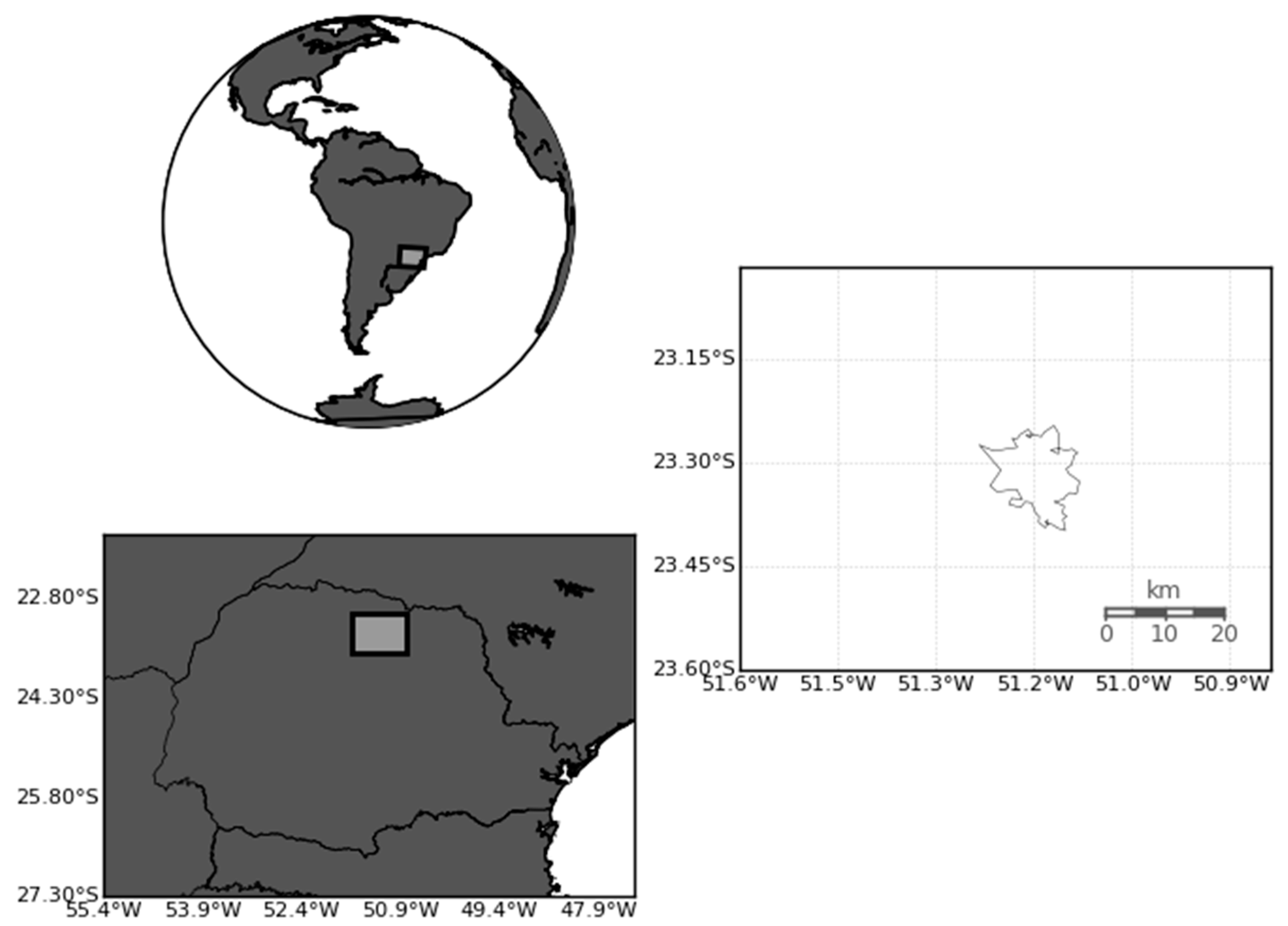
The model was adjusted to have three nesting grids, with horizontal homogeneous spacing grid of 9, 3 and 1 km, centered in the city of Londrina (near −23.3°, −51.1°; Figure 2). In the vertical level, it was set 35 sigma levels, with the top in 50 hPa (about 20 km height). Table 1 shows the parameterizations used in this study. The land and soil use in all simulation are from Moderate-Resolution Imaging Spectroradiometer (MODIS), with horizontal spacing grid of 500 m [39].

3. Results

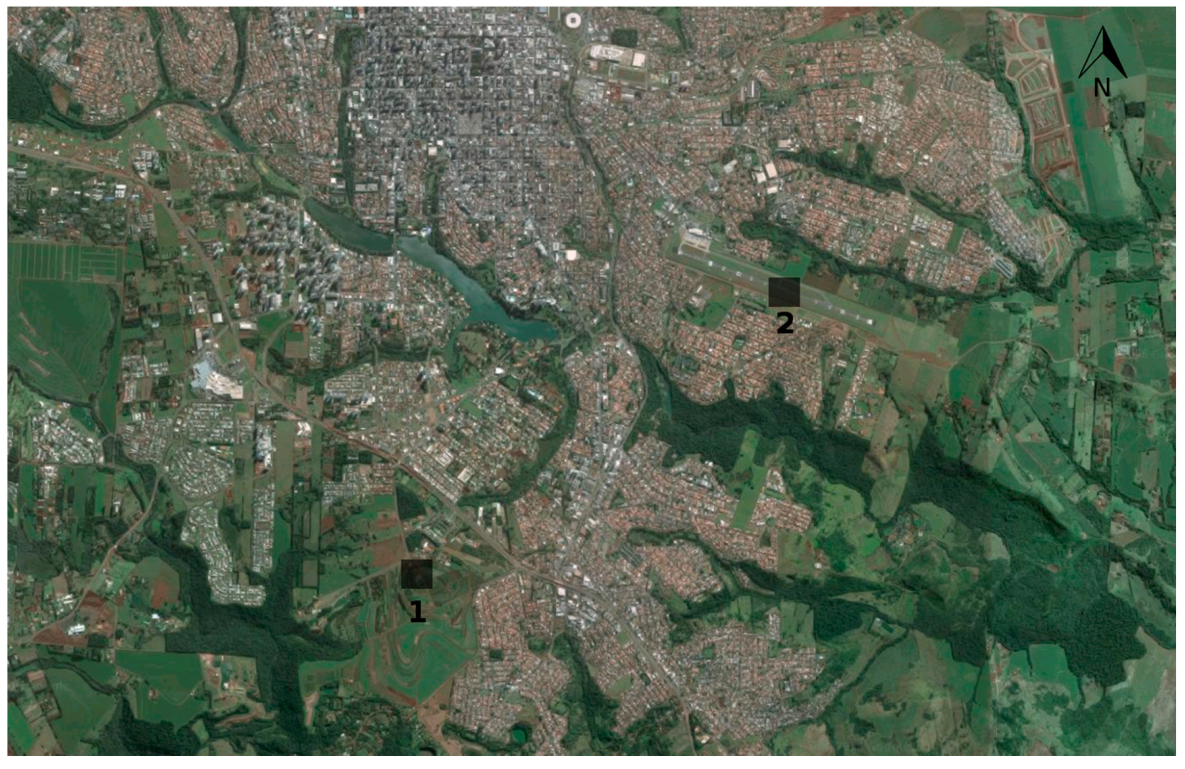
To evaluate the model, statistical indexes were calculated using data from observational surface stations spread inside the Londrina. Two surfaces observation stations were used to evaluate the model. The first one is the SIMEPAR (Meteorological System of Paraná), located at 23.36° S and longitude 51.1647° W, and the second is the METAR data from the airport (23.33° S, 51.14° W). Figure 3 presents the location of both stations.
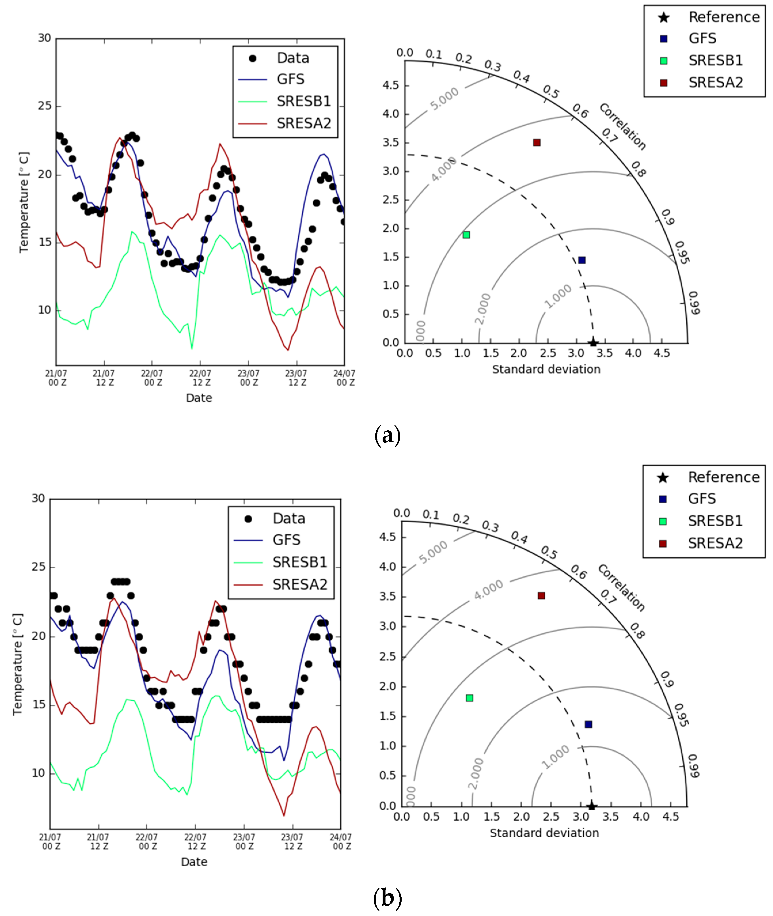
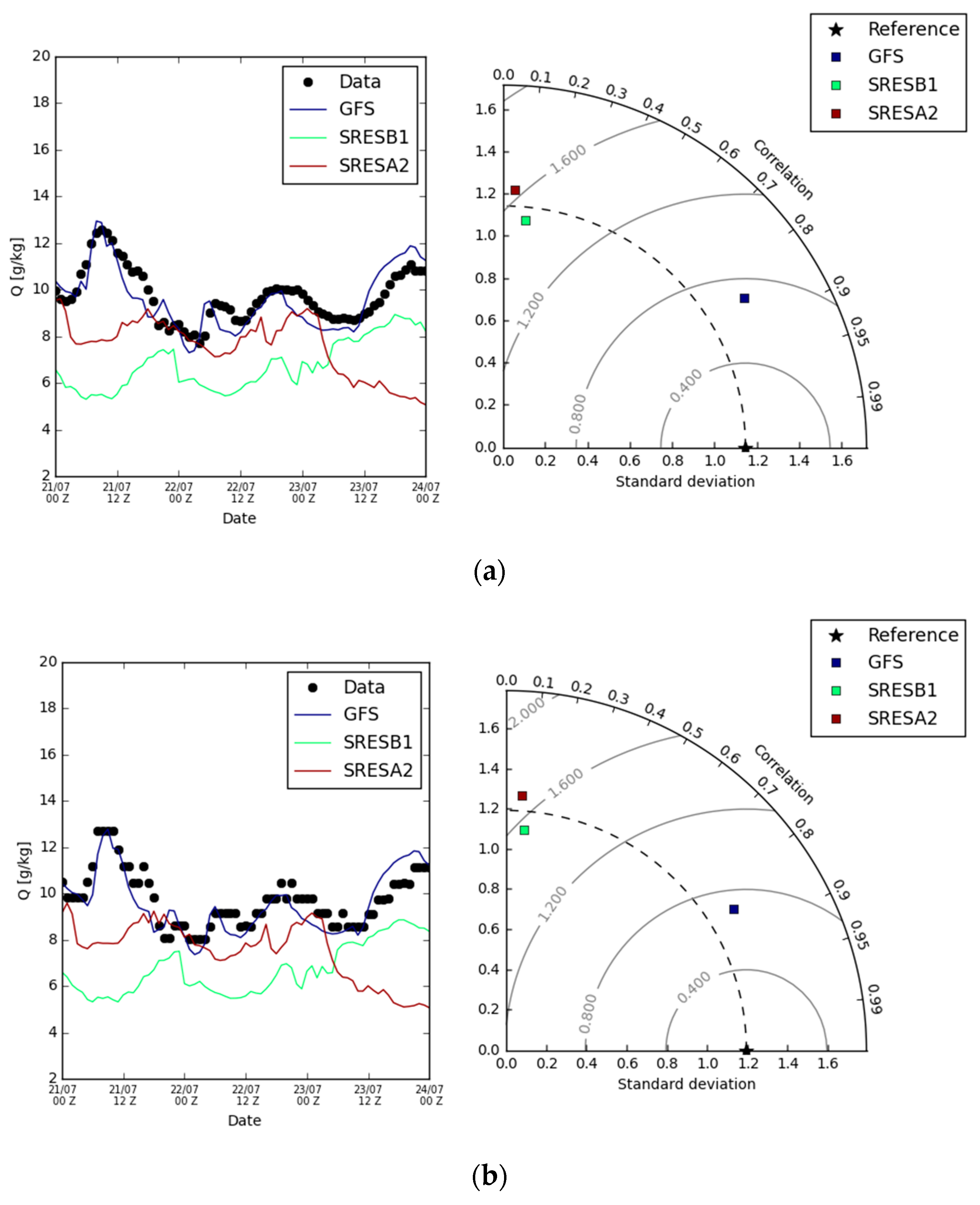
To evaluate the model, the normalized Taylor Diagram [48] for temperature and specific humidity was analyzed for both stations and for each different input data, where SRESA2 is the simulation with A2 scenario as input, SRESB1 is with B1 scenario and GFS is the simulation with GFS as input data. Figure 4 shows the results for temperature at 2 m and Figure 5, the results for specific humidity at 2 m.
Comparing the correlations of the model output for temperature with the observations for both datasets (SIMEPAR and METAR), a substantial higher correlation is notable for the GFS (r = 0.93 for METAR and 0.92 for SIMEPAR), while for the sustainable case (SRESB1) have the low values (r = 0.61 for METAR and r = 0.59 for SIMEPAR). For SRESA2 case, the correlation has higher values than the SRESB1, but not adequate as GFS (r = 0.65 for METAR and 0.64 for SIMEPAR). For RMS (Root Mean Square), the GFS simulation has 1.37, while SRESB1 has 2.74 and SRESA2 is 3.62 for METAR station. For SIMEPAR station, the RMS for GFS is 1.46, while SRESB1 is 2.92 and SRESA2 is 3.66. For standard deviation, the value obtained for observational data is 3.18, while for GFS is about 3.40, SRESB1 is 2.14 and SRESA2 is 4.23 for METAR. For SIMEPAR, the standard deviation for observational data is 3.30, while for GFS simulation is 3.41, SRESB1 is 2.18 and SRESA2, 4.20. The result shows that GFS has a better skill, while the A2 scenarios has closer values to the GFS.
For specific humidity, when comparing the correlations of the model output with the observations for both datasets (SIMEPAR and METAR), a better correlation is notable for the GFS (r = 0.85 for both METAR and SIMEPAR), while for the sustainable case (SRESB1) have the low values (r = 0.08 for METAR and r = 0.1 for SIMEPAR). For SRESA2 case, the correlation has higher values than the SRESB1, but not adequate as GFS (r = 0.06 for METAR and 0.04 for SIMEPAR). For RMS, the GFS simulation has 0.70, while SRESB1 has 1.69 and SRESA2 is 1.80 for METAR station. For SIMEPAR station, the RMS for GFS is 0.71, while SRESB1 is 1.65 and SRESA2 is 1.71. For standard deviation, the value obtained for observational data is 1.19, while for GFS is about 1.33, SRESB1 is 1.10 and SRESA2 is 1.27 for METAR. For SIMEPAR, the standard deviation for observational data is 1.14, while for GFS simulation is 1.34, SRESB1 is 1.08 and SRESA2, 1.22. Like for temperature, the results shows that GFS has a better skill, while the A2 scenarios has closer values of the indexes to the GFS, comparing with the B1 scenarios.
During the period of simulation, the highest intensity of UHI happens about 18 Z (15 Local Time) at 22 July. Figure 6 presents the maps of temperature at 2 m for all simulations at this period. The difference of temperature at urban area and the rural adjacent area for GFS simulation is about 0.5 °C (Figure 6c), with a mean temperature for urban area at 18 °C and 17.5 °C for rural area. For SRESB1 simulation (Figure 6b), both temperature for urban and rural area decreases, with mean magnitudes of 16 °C and 14 °C, respectively. In this case, the UHI intensity grows to 2 °C. In the SRESA2 simulation (Figure 6a), the mean of the temperature difference is lower than that considered in the SRESB1 simulation, reaching an intensity of 1 °C. In spite of this, it is important to note that the increase in temperature occurs in both the urban area (22.5 °C average) and the rural area (21.5 °C average), with similar peaks in both regions (23.5 °C).
The pattern of the wind also changes in the three figures. While an east wind is expected at this time of year (Figure 6c), in the case of the SRESB1 simulation a southern wind is noted. Meanwhile, in the SRESA2 simulation, besides the wind being of the west, a greater convergence happens in the incidence of urban region. It is also remarkable how much higher warming in the rural region influences the wind field in this simulation.
Fields of specific humidity at 2 m for all simulations at 18 Z for 22 July are shown in Figure 7. The SRESB1 simulation has drier values of humidity than SRESA2 and GFS in the urban area. At this time, the specific humidity is about 7.5 g/kg for SRESA2 simulation, while for GFS is about 9 g/kg. The SRESB1 simulation has lower values of specific humidity in the urban area, about 5.5 g/kg, it values are closer to the rural area (about 6.5 g/kg). It can be cleared that, regardless of the future scenario simulated, the air could be drier than current situation in the region, urban areas and rural areas, which could be implications on production of foods. This drier rural area was also found by Hamdi et al. (2015) [7], which has an important role in the UHI development for Paris in the A1B scenario (considered balanced).
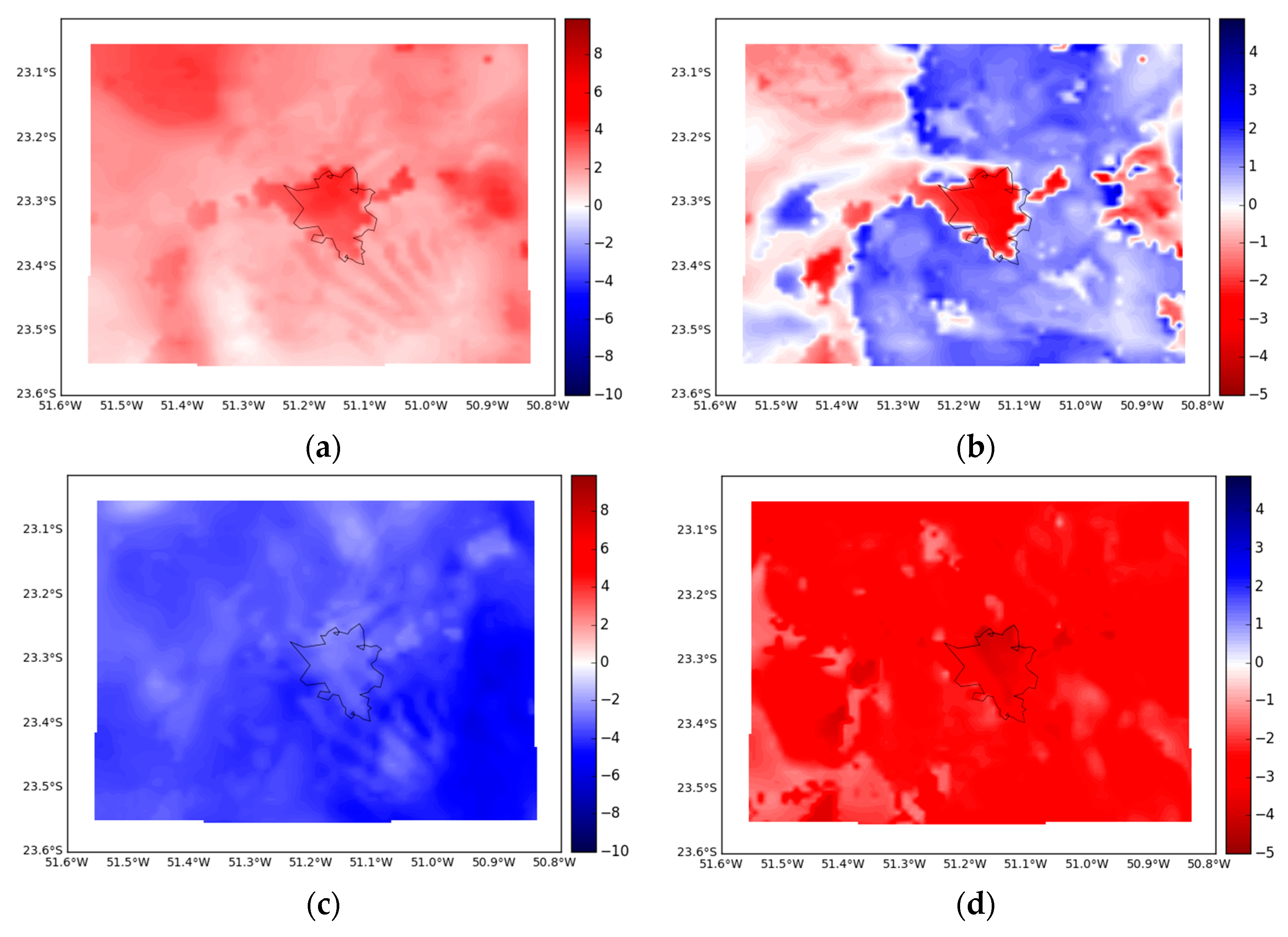
The impact of climate scenarios is better visualized when the difference with the actual situation (considered the simulation with the GFS as input) is analyzed. Figure 8 shows the result of these differences. As previously described and observed in the Figure 8, the most pessimistic scenario (A2) presents a higher temperature in both rural and urban areas (Figura 8a). In this case, the urban area is drier than the actual situation (Figure 8b), while the rural area is more humid, with a difference of up to 3.5 g/kg of specific humidity. However, the more sustainable scenario (B1) has a lower temperature compared to the real situation (Figure 8c), but both the urban and rural areas are drier than the GFS simulation (Figure 8d). This differences has influence in the lower intensity of UHI for B1 scenario.

4. Discussion and Conclusions

This work presented an analysis of the physical processes in the formation and intensity of the UHI for the city of Londrina, using 3 dynamically downscalled scenarios: the present one—through the simulation with the GFS data as input; the SRESA2—using the A2 climate scenario, considered the most pessimistic; and SRESB1—using scenario B1, considered the most sustainable. The simulations were carried out for July 2015, a winter period, with no clouds or rain condition, considered a projection for the IPCC climate scenarios.
Considering the simulation of GFS, and based on the evaluation of the model, it can be noted that the current situation for both temperature and specific humidity at 2 m, is more similar to presented by the A2 scenario than the B1. All SRESA2 indexes was closer to GFS than SRESB1. It can be seen in the peak of temperature at 22 July at 15 Z, when temperature values from SRESA2 are closer to than SRESB1 temperature values.
It is remarkable how much the physical processes involved in the atmosphere influence the formation and intensity of the UHI. Even considering the situation more sustainable, the intensity of the realistic UHI was similar to the case of the most pessimistic situation. This is due to the fact that the rural region of the B1 case is drier than the A2 simulation. Thus, this has an influence on the energy budget at surface, confirming the high intensity of the UHI for B1 simulation. This is similar to that found in the literature. This future scenario downscaled that presents a drier rural area, could be an implications in food production in this important agricultural area of Brazil. The decrease on humidity affects directly the formation and the intensity of UHI. The higher value of the A2 scenarios affects the wind pattern at local scale, probably influencing on the pollutants dispersion. The greater convergence at urban area can configure a maintenance of high levels of poor air quality. Finally, the dynamical downscaling of future scenarios is an important tool to analyses the impact of it in a local scale.
Further research to provide new insights into the UHI formation in Londrina is underway. It is expected to carry out future simulations (for 2020, 2030, 2040 and 2050), using future projections of urban land use and occupation based on the population and economic projections. In addition, simulations using the chemical version of the model will also be performed based on projections of vehicle use and industrial emissions.

Author Contributions

M.V.B.d.M., V.V.U.G., L.D.M. and J.A.M. conceived, designed and performed the modeling experiments. All authors have read and agreed to the published version of the manuscript.

Acknowledgments

The author Marcos Vinicius Bueno de Morais wants to thank CAPES (Coordenacão de Aperfeiçoamento de Pessoal de Nível Superior—process 88887.094508/2015-00) for the financial support of this work. Co-author Leila Droprinchinski Martins acknowledgement CNPq (process 404104/2013-4 and 303491/2015-9) for financial support. We also thank the SIMEPAR for providing meteorological data. Finally, the authors thank Yannick Copin for sharing Taylor Diagram script.

Conflicts of Interest

The authors declare no conflict of interest.

Abbreviations

The following abbreviations are used in this manuscript:
1. UHI2. Urban Heat Island
3. WRF4. Weather Research and Forecast
5. GFS6. Global Forecast System
7. CCSM38. Community Climate System Model Version 3
9. IPCC10. Intergovernmental Panel on Climate Change
11. SRES12. Special Report of Emission Scenarios
13. SIMEPAR14. Meteorological System of Paraná (Sistema Meteorológico do Paraná, in portuguese)
15. SO216. Sulfur dioxide
17. CO18. Carbon monoxide
19. NOx20. Nitrogen oxides
21. NMHC22. Non-methane hydrocarbons
23. SRESA224. Simulation with A2 scenario from CCSM3
25. SRESB126. Simulation with B1 scenario from CCSM3

References

  1. Intergovernmental Panel on Climate Change (IPCC). Climate Change 2007: The Physical Science Basis, Contribution of Working Group I. In Fourth Assessment Report of the Intergovernmental Panel on Climate Change; Cambridge University Press: Cambridge, UK; New York, NY, USA, 2007; 996p. [Google Scholar]
  2. Revi, A.; Satterthwaite, D.E.; Aragón-Durand, F.; Corfee-Morlot, J.; Kiunsi, R.B.R.; Pelling, M.; Roberts, D.C.; Solecki, W.; da Silva, J.; Dodman, D.; et al. Urban areas. In Climate Change 2014: Impacts, Adaptation, and Vulnerability. Part A: Global and Sectoral Aspects. Contribution of Working Group II to the Fifth Assessment Report of the Intergovernmental Panel on Climate Change; Field, C.B., Barros, V.R., Dokken, D.J., Mach, K.J., Mastrandrea, M.D., Bilir, T.E., Chatterjee, M., Ebi, K.L., Estrada, Y.O., Genova, R.C., et al., Eds.; Cambridge University Press: Cambridge, UK; New York, NY, USA, 2015; pp. 535–612. [Google Scholar]
  3. Ribeiro, W.C. Impact of the climate changes in the cities of Brazil (Impacto das mudanças climáticas em cidades no Brasil). Parcer. Estratég. 2008, 27, 293–321. (In Portuguese) [Google Scholar]
  4. Rosenzweig, C.; Solecki, W.; Hammer, S.A.; Mehrotra, S. Cities lead the way in climate-change action. Nature 2010, 467, 909–911. [Google Scholar] [CrossRef] [PubMed]
  5. Nakicenovic, N.; Alcamo, J.; Davis, G.; Vries, B.; Fenhann, J.; Gaffin, S.; Kermeth, G.; Amulf, G.; Jung, T.Y.; Kram, T.; et al. Special Report on Emission Scenarios, Published for the Intergovernamental Panel on Climate Change; Cambridge University Press: New York, NY, USA, 2000; 608p. [Google Scholar]
  6. Früh, B.; Becker, P.; Deutschlander, T.; Hessel, J.D.; Kossman, M.; Mieskes, I.; Namyslo, J.; Roos, M.; Sievers, U.; Steigerwald, T.; et al. Estimation of Climate-Change Impacts on the Urban Heat Load Using an Urban Climate Model and Regional Climate Projections. J. Appl. Meteorol. 2011, 50, 167–184. [Google Scholar] [CrossRef]
  7. Hamdi, R.; Giot, O.; De Troch, R.; Deckmyn, A.; Termonia, P. Future Climate of Brussels and Paris for the 2050s under A1B scenario. Urban Clim. 2015, 12, 160–182. [Google Scholar] [CrossRef]
  8. Parker, A.S.; Kusaka, H.; Yamagata, Y. Assessment of the Impact of Metropolitan-Scale Urban Planning Scenarios on the Moist Thermal Environment under Global Warming: A Study of the Tokyo Metropolitan Area Using Regional Climate Modeling. Adv. Meteorol. 2015, 2015, 693754. [Google Scholar]
  9. Lemonsu, A.; Viguié, V.; Daniel, M.; Masson, V. Vulnerability to heat waves: Impact of urban expansion scenarios on urban heat island and heat stress in Paris (France). Urban Clim. 2015, 14, 586–605. [Google Scholar] [CrossRef]
  10. Semenza, J.C.; Mccullough, J.; Flanders, W.D.; Mcgeehin, M.A.; Rubin, C.H.; Lumpkin, J.R. Excess hospital admissions during the 1995 heat wave in Chicago. Am. J. Prev. Med. 1999, 16, 269–277. [Google Scholar] [CrossRef]
  11. Kalnay, E.; Cai, M. Impact of urbanization and land-use change on climate. Nature 2003, 423, 528–531. [Google Scholar] [CrossRef]
  12. Oke, T.R. Boundary Layer Climates, 2nd ed.; Cambridge University Press: New York, NY, USA, 1988; 435p. [Google Scholar]
  13. Arnfield, A.J. Two decades of Urban Climate Research: A review of Turbulence Exchanges of Energy and Water, and the Urban Heat Island. Int. J. Climatol. 2003, 23, 1–26. [Google Scholar] [CrossRef]
  14. Atkinson, B.W. Numerical Modelling of Urban Heat-Island Intensity. Bound. Layer Meteorol. 2003, 109, 285–310. [Google Scholar] [CrossRef]
  15. Montálvez, J.P.; Rodriguéz, A.; Jiménez, J.I. A study of the urban heat island of Granada. Int. J. Climatol. 2000, 20, 899–911. [Google Scholar] [CrossRef]
  16. Morris, C.J.G.; Simmonds, I. Associations between varying magnitudes of the urban heat island and the synoptic climatology in Melbourne, Australia. Int. J. Climatol. 2000, 20, 1931–1954. [Google Scholar] [CrossRef]
  17. Li, D.; Bou-Zeid, E. Synergistic interactions between urban heat islands and heat waves: The impact in cities is larger than the sum of its parts. J. Appl. Meteorol. 2013, 52, 2051–2064. [Google Scholar] [CrossRef]
  18. Dabbert, W.F.; Hales, J.; Zubrick, S.; Crook, A.; Mueller, C.; Krajewski, W.; Doran, J.C.; Mueller, C.; King, C.; Keener, R.N.; et al. Forecast Issues in the Urban Zone: Report of the 10th Prospectus Development Team of the U.S. Weather Research Program. Bull. Am. Meteorol. Soc. 2000, 81, 2047–2064. [Google Scholar] [CrossRef]
  19. Freitas, E.D. Circulações Locais em São Paulo e sua Influência na Dispersão de Poluentes. 157 f. Ph.D. Thesis, Atmospheric Science Department, University of São Paulo, São Paulo, Brazil, 2003. [Google Scholar]
  20. Ketzel, M.; Berkowicz, R.; Muller, W.; Lohmeyer, A. Dependence of street canyon concentrations on above roof wind speed—Implications for numerical modelling. Int. J. Environ. Pollut. 2002, 17, 356–366. [Google Scholar] [CrossRef]
  21. Urbina Guerrero, V.V. Características das Circulações Locais em Regiões Metropolitanas do Chile Central. 113 f. Master’s Thesis, Instituto de Astronomia, Geofísica e Ciências Atmosféricas, Universidade de São Paulo, São Paulo, Brazil, 2010. [Google Scholar]
  22. Britter, R.; Hanna, S.R. Flow and dispersion in urban areas. Annu. Rev. Fluid Mech. 2003, 35, 469–496. [Google Scholar] [CrossRef]
  23. Harman, I.N. The Energy Balance of Urban Areas. 157 f. Ph.D. Thesis, University of Reading, London, UK, 2003. [Google Scholar]
  24. Marengo, J.A.; Ambrizzi, T. Use of regional climate models in impacts assessments and adaptations studies from continental to regional and local scales: The CREAS (Regional Climate Change Scenarios for South America) initiative in South America. In Proceedings of the 8th International Conference on Southern Hemisphere Meteorology and Oceanography (ICSHMO), Foz do Iguaçu, Brazil, 24–28 April 2006; pp. 291–296. [Google Scholar]
  25. Marengo, J.A.; Jones, R.; Alves, L.M.; Valverde, M.C. Future change of temperature and precipitation extremes in South America as derived from the PRECIS regional climate modeling system. Int. J. Climatol. 2009, 29, 2241–2255. [Google Scholar] [CrossRef]
  26. Reboita, M.S.; Rocha, R.P.; Dias, C.G.; Ynoue, R.Y. Climate Projections for South America: RegCM3 Driven by HadCM3 and ECHAM5. Adv. Meteorol. 2014, 2014, 376738. [Google Scholar] [CrossRef]
  27. IBGE 2014: Data of South and Southeast Region of Brazil. Available online: http://www.ibge.gov.br/ (accessed on 12 May 2017).
  28. Capucim, M.N.; Brand, V.S.; Machado, C.B.; Martins, L.D.; Allasia, D.G.; Homann, C.T.; Freitas, E.D.; Silva Dias, M.A.F.; Andrade, M.F.; Martins, J.A. South America land use and land cover assessment and preliminary analysis of their impacts on regional atmospheric modeling studies. IEEE J. Sel. Top.Appl. 2014, 8, 1185–1198. [Google Scholar] [CrossRef]
  29. Skamarock, W.C.; Klemp, J.B.; Dudhia, J.; Gill, D.O.; Barker, D.M.; Duda, M.G.; Huang, X.Y.; Wang, W.; Powers, J.G. A Description of the Advanced Research WRF Version 3; NCAR Technical Note; NCAR/TN-475+STR: Boulder, CO, USA, 2008. [Google Scholar]
  30. Collins, W.D.; Bitz, C.M.; Blackmon, M.L.; Bonan, G.B.; Bretherton, C.S.; Carton, J.A.; Chang, P.; Doney, S.C.; Hack, J.J.; Henderson, T.B.; et al. The Community Climate System Model Version 3 (CCSM3). J. Clim. 2006, 19, 2122–2143. [Google Scholar] [CrossRef]
  31. Collins, W.D.; Rasch, P.J.; Boville, B.A.J.; McCaa, J.R.; Williamson, D.L.; Kiehl, J.T.; Briegleb, B.; Bitz, C.; Lin, S.J. Description of the NCAR Community Atmosphere Model (CAM3); NCAR Technical Note; NCAR/TN-464_STR: Boulder, CO, USA, 2004. [Google Scholar]
  32. Oleson, K.; Dai, Y.; Bonan, G.B.; Bosilovichm, M.; Dickinson, R.; Dirmeyer, P.; Hoffman, F.; Houser, P.; Levis, S.; Niu, G.Y.; et al. Technical Description of the Community Land Model (CLM); NCAR Technical Report; NCAR/TN-461+STR: Boulder, CO, USA, 2004. [Google Scholar]
  33. Dickinson, R.E.; Oleson, K.W.; Bonan, G.; Hoffman, F.; Thornton, P.; Vertenstein, M.; Yang, Z.L.; Zeng, X. The Community Land Model and its climate statistics as a component of the Community Climate System Model. J. Clim. 2006, 19, 2302–2324. [Google Scholar] [CrossRef]
  34. Briegleb, B.P.; Bitz, C.M.; Hunke, E.C.; Lipscomb, W.H.; Holland, M.M.; Schramm, J.L.; Moritz, R.E. Scientific Description of the Sea Ice Component in the Community Climate System Model, Version Three. NCAR Technical Report; NCAR/TN-463STR: Boulder, CO, USA, 2004. [Google Scholar]
  35. Smith, R.D.; Gent, P.R. Reference Manual for the Parallel Ocean Program (POP), Ocean Component of the Community Climate System Model (CCSM2.0 and 3.0). NCAR Technical Report; LA-UR-02-2484: Boulder, CO, USA, 2002. [Google Scholar]
  36. Mazzoli, C.R. Estudo Numérico da Influência das Mudanças Climáticas e das Emissões Urbanas no Ozônio Troposférico da Região Metropolitana de São Paulo. 162 f. Ph.D. Thesis, University of São Paulo, São Paulo, Brazil, 2003. [Google Scholar]
  37. Kanamitsu, M.; Alpert, J.C.; Campana, K.A.; Caplan, P.M.; Deaven, D.G.; Iredell, M.; Katz, B.; Pan, H.L.; Sela, J.; White, G.H. Recent changes implemented into the global forecast system at NMC. Weather Forecast. 1991, 6, 425–436. [Google Scholar] [CrossRef]
  38. Daley, R. Atmospheric Data Analysis; Cambridge Press: New York, NY, USA, 1991; pp. 1–457. [Google Scholar]
  39. Schneider, A.; Friedl, M.A.; Potere, D. A new map of global urban extent from MODIS data. Environ. Res. Lett. 2009, 4, 044003. [Google Scholar] [CrossRef]
  40. Kessler, E. On the Distribution and Continuity of Water Substance in Atmospheric Circulation; American Meteorological Society: Boston, MA, USA, 1969; Volume 10, 88p. [Google Scholar]
  41. Grell, G.A.; Freitas, S.R. A scale and aerosol aware stochastic convective parameterization for weather and air quality modeling. Atmos. Chem. Phys. 2014, 14, 5233–5250. [Google Scholar] [CrossRef]
  42. Zhang, D.; Anthes, R.A. A High-Resolution Model of the Planetary Boundary Layer—Sensitivity Tests and Comparisons with SESAME-79 Data. J. App. Meteorol. 1982, 21, 1594–1609. [Google Scholar] [CrossRef]
  43. Chen, F.; Dudhia, J. Coupling an advanced land surface-hydrology model with the Penn State-NCAR MM5 modeling system. Part I: Model implementation and sensitivity. Mon. Weather Rev. 2001, 129, 569–585. [Google Scholar] [CrossRef]
  44. Kusaka, H.; Kimura, F. Coupling a single-layer urban canopy model with a simple atmospheric model: Impact on urban heat island simulation for an idealized case. J. Meteorol. Soc. Jpn 2004, 82, 67–80. [Google Scholar] [CrossRef]
  45. Hong, S.; Noh, Y.; Dudhia, J. A new vertical diffusion package with explicit treatment of entrainment processes. Mon. Weather Rev. 2006, 134, 2318–2341. [Google Scholar] [CrossRef]
  46. Dudhia, J. Numerical Study of Convection Observed during the Winter Monsoon Experiment Using a Mesoscale Two—Dimensional Model. J. Atmos. Sci. 1989, 46, 3077–3107. [Google Scholar] [CrossRef]
  47. Mlawer, E.J.; Taubman, S.J.; Brown, P.D.; Iacono, M.J.; Clough, S. A Radiative transfer for inhomogeneous atmospheres: RRTM, a validated correlated-k model for the longwave. J. Geophys. Res. Atmos. 1997, 102, 16663–16682. [Google Scholar] [CrossRef]
  48. Taylor, K.E. Summarizing multiple aspects of model performance in a single diagram. J. Geophys. Res. 2001, 106, 7183–7192. [Google Scholar] [CrossRef]
Figure 1. Future projection of global carbon dioxide emission for the (a) A2 and (b) B1 scenarios from SRES. From Nakicenovic et al. (2000) [5].
Proceedings 01 00106 g001
Figure 2. Localization of the city of Londrina. On the right map, the grid with more resolution. The shape map on this figure is the urban area of Londrina.
Proceedings 01 00106 g002
Figure 3. Localization of the meteorological station from the city of Londrina. Number 1 is the SIMEPAR station, while number 2 is the METAR station.
Proceedings 01 00106 g003
Figure 4. Evolution of temperature (left column) and Taylor diagram (right column) for (a) SIMEPAR and (b) Londrina Airport METAR data stations. Blue line is the simulation with GFS as input and boundary conditions, green line is the simulation with B1 scenario and red line is the simulation with A2 scenario. Both are output from CCSM3 model.
Proceedings 01 00106 g004
Figure 5. Evolution of specific humidity (left column) and Taylor diagram (right column) for (a) SIMEPAR and (b) Londrina Airport METAR data stations. Blue line is the simulation with GFS as input and boundary conditions, green line is the simulation with B1 scenario and red line is the simulation with A2 scenario. Both are output from CCSM3 model.
Proceedings 01 00106 g005
Figure 6. Air temperature at 2 m (in °C) for 18 Z at 22 July 2015 for simulation with (a) SRESA2; (b) SRESB1 and (c) GFS simulations. Black arrow is the wind velocity intensity at 10 m.
Proceedings 01 00106 g006
Figure 7. Specific humidity at 2 m (in g/kg) for 18 Z at 22 July 2015 for simulation with (a) GFS; (b) SRESB1 and (c) SRESA2 simulations.
Proceedings 01 00106 g007
Figure 8. Difference of air temperature at 2 m (in °C) for (a) SRESA2 and GFS; (c) SRESB1 and GFS; and difference of specific humidity at 2 m (in g/kg) (b) SRESA2 and GFS and (d) SRESB1 and GFS for 18 Z at 22 July 2015.
Proceedings 01 00106 g008
Table 1. Physical parametrizations used in this study.
PhysicsSchemes
MicrophysicsKessler Scheme [40]
CumulusGrell-Freitas [41]
Surface LayerMM5 [42]
Soil-LandNoah LSM [43]
UrbanUCM [44]
Boundary LayerYounsei University Scheme [45]
Shortwave RadiationDudhia [46]
Longwave RadiationRRTM [47]
Publisher’s Note: MDPI stays neutral with regard to jurisdictional claims in published maps and institutional affiliations.