A Numerically Exact Method for Dissipative Dynamics of Qubits ^†

Abstract

We propose a numerical technique suitable for simulating the dynamics of reduced density matrix of a qubit interacting with its environment. Our approach, based on a combination of short-iterative Lanczos method (SIL) and a flexible truncation scheme, allows to include in the physical description multiple-excitation processes, beyond weak coupling and Markov approximations. We perform numerical simulations of two different model Hamiltonians, that are relevant in the field of adiabatic quantum computation (AQC), and we show that our technique is able to recover the correct thermodynamic behavior of the qubit-bath system, from weak to intermediate coupling regime.

1. Introduction

The correct understanding of dissipation and decoherence in open quantum systems is of crucial importance for the realization of quantum information devices. The spin boson model (SBM), which describes a two level system (TLS) interacting with a bosonic bath at thermodynamic equilibrium, is a well-known prototype of an open quantum system [1]. In recent years, there has been a renewed interest in studying the role of decoherence in AQC, a field that regained momentum since the first experimental demonstration of the D-Wave machine [2]. A number of different techniques have been developed in order to describe the out-of-equilibrium dynamics of these system. Among them, the adiabatic time-dependent generalization of Quantum Master Equations (QMEs), such as the Gorini-Kossakowski-Sudarshan-Lindblad equation [3,4] (Lindblad equation for brevity), which rely on the Born-Markov (weak qubit-bath coupling) and rotating wave approximations. As claimed in the recent literature [5,6], the interaction with a thermal bath is not necessarily detrimental to the success of AQC: in this scenario, multiple-excitation processes may become relevant and a purely Born-Markov approach might fail to reproduce the correct physical behavior of these systems.

In this work, we propose an exact numerical technique aimed at providing an alternative tool to study decoherence and dissipation in open quantum systems. It combines a flexible truncation of the Hilbert space of the bosonic bath and SIL method, thus allowing to compute the dynamics of the whole $\mathrm{qubit}+\mathrm{bath}$ quantum state. We test the predictions of our method by analyzing two different model Hamiltonians of a TLS interacting with a bath, and compare our results with conventional approaches based on the Lindblad QME.

2. Materials and Methods

2.1. Model Hamiltonian

We focus on the study of a TLS, i.e., a qubit interacting with an external bath at thermodynamic equilibrium. The Hamiltonian of the $\mathrm{qubit}+\mathrm{bath}$ system can be written as $H\left(t\right)=H_S\left(t\right)+H_B+H_I$, where $H_S\left(t\right)$ is a time-dependent Hamiltonian describing the evolution of the isolated qubit, $H_B$ is the bath Hamiltonian and $H_I$ is the time-independent interaction term between the qubit and the bath. We choose as the computational basis of the qubit the set of eigenstates of the operator ${\sigma }_z$ and take the operator $H_S\left(t\right)$ as a real and symmetric operator having the form $H_S\left(t\right)=-\mathsf{\Gamma }\left(t\right){\sigma }_x-\epsilon \left(t\right){\sigma }_z$, where ${\sigma }_{x/z}$ are spin-$1/2$ Pauli operators, $\mathsf{\Gamma }\left(t\right)$ is a transverse field and $\epsilon \left(t\right)$ is an energy bias between the two computational basis states. We model the bath as an ensemble of harmonic oscillators, and the bath Hamiltonian $H_B$ reads: $H_B={\sum }_k{\omega }_k{b}_k^{†}{b}_k$; $b_m^{†}\left(b_m\right)$ are the usual creation (annihilation) bosonic operators obeying to $\left[b_l{b}_m^{†}\right]={\delta }_{lm}$, and ${\omega }_k$ is the frequency of the $k^{\mathrm{th}}$ mode. We take the qubit as linearly coupled to the environment, along the longitudinal $\widehat{z}$ direction, i.e., $H_I={\sigma }_z{\sum }_k{g}_k(b_k+b_k^{†})$. Here, $g_k$ is the coupling energy between the qubit and the $k^{\mathrm{th}}$ bosonic mode. We characterize the coupling with the bath by choosing the bath spectral density as $J\left(\omega \right)={\sum }_k{g}_k^2\delta (\omega -{\omega }_k)=\eta \frac{{\omega }^s}{{\omega }_{\mathrm{c}}^{s-1}}\mathsf{\Theta }({\omega }_{\mathrm{c}}-\omega )$, where we have taken the continuum limit, fixed a high-frequency sharp cut-off ${\omega }_{\mathrm{c}}$ and introduced the dimensionless coupling strength $\eta$. The exponent s characterizes dissipation and distinguishes between Ohmic ($s=1$), sub-Ohmic ($s<1$) and super-Ohmic ($s>1$) environments.

2.2. Short-Iterative Lanczos

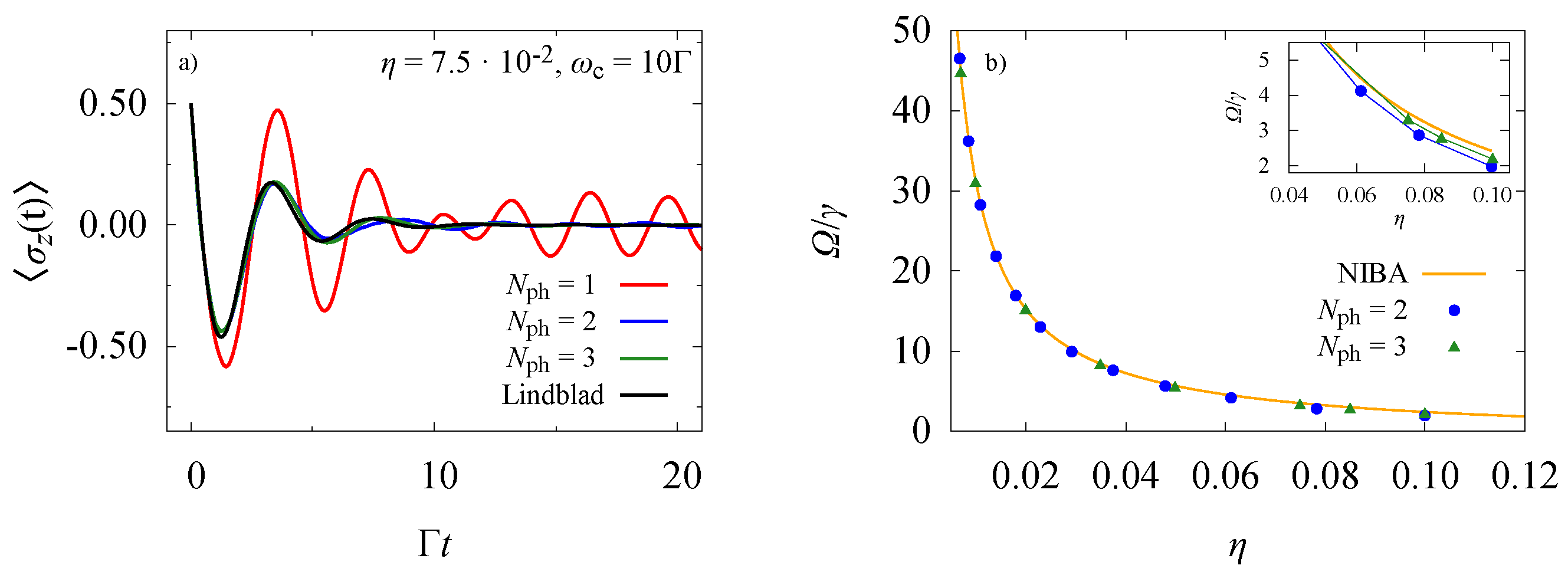
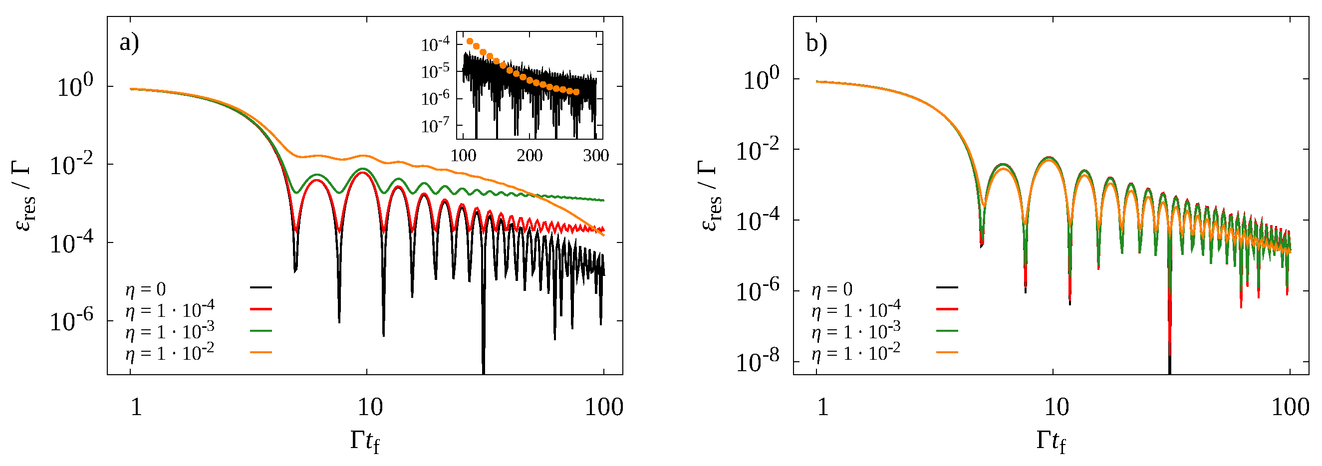
Our goal is to compute the dynamics of the whole $\mathrm{qubit}+\mathrm{bath}$ system state $\rho \left(t\right)=U(t,t_0)\rho \left(t_0\right)U^{†}(t,t_0)$, starting from an initial state $\rho \left(t_0\right)={\rho }_S\left(t_0\right)\otimes {\rho }_B$, where ${\rho }_{S}and{\rho }_B$ are the density matrices of the reduced system and the bath, respectively. To this end, we first perform a discretization of the bath modes ${\omega }_k$, taking them as equally spaced: ${\omega }_k=k{\omega }_{\mathrm{c}}/M$, with $k=1,\cdots ,M$. Then, we perform a truncation of the bath Hilbert space $\left\{|n_1,n_2,\cdots ,n_M\rangle \right\}$ in the following way: we fix the absolute maximum number $N_{\mathrm{ph}}$ of bosonic excitations with respect to the thermodynamic equilibrium values occupation numbers $n_k^{\mathrm{eq}}$, and include in the physical description only the basis states with $\mathsf{\Delta }{n}_k=n_k-n_k^{\mathrm{eq}}=0,\pm 1,\pm 2,\cdots ,\pm N_{\mathrm{ph}}$, with ${\sum }_k\left|\mathsf{\Delta }{n}_k\right|\le N_{\mathrm{ph}}$. Further, we divide the entire time interval in sub-intervals of fixed length dt: for each sub-interval $[t,t+\mathrm{d}t]$, we project the total Hamiltonian evaluated at midpoint $H(t+\mathrm{d}t/2)$ onto the Krylov subspace $\mathcal{K}=\{|\mathsf{\Psi }\left(t\right)\rangle ,H|\mathsf{\Psi }\left(t\right)\rangle ,\cdots ,H^n|\mathsf{\Psi }\left(t\right)\rangle \}$, where $|\mathsf{\Psi }\left(t\right)\rangle$ is the whole system+bath ket state at time t and n is the minimum number of iterations needed to achieve convergence. Once the reduction to this subspace is obtained, we can apply exact diagonalization techniques to the reduced n-dimensional Hamiltonian $\tilde{H}=PHP$ and directly compute the evolution operator $\tilde{U}(t+\mathrm{d}t,t)\simeq exp[-i\tilde{H}(t+\mathrm{d}t/2)\mathrm{d}t]$.

It follows that our method allows us to compute the $\mathrm{qubit}+\mathrm{bath}$ ket state at any final time, and the dynamics of every observable regarding both the qubit and the bath can be readily obtained. This technique introduces a clear advantage over conventional methods which look only at the reduced dynamics of the qubit. In addition, it allows to describe the physics of these systems beyond the Born-Markov scenario, and a better control over the approximations can be achieved in comparison with conventional QMEs [7].

3. Results

3.1. Spin-Boson Model

We fix $\epsilon \left(t\right)=0$ and the transverse field equal to a constant, i.e., $\mathsf{\Gamma }\left(t\right)=\mathsf{\Gamma }$, and study the dynamics of the unbiased SBM. We choose the cut-off frequency ${\omega }_{\mathrm{c}}=10\mathsf{\Gamma }$, the coupling parameter $\eta$ in the range $\eta =5\times {10}^{-4}\mathrm{to}1\times {10}^{-1}$, and focus on the case of Ohmic dissipation. We report the results of the dynamics of the expectation value $\langle {\sigma }_z\left(t\right)\rangle$ at $T=0$ computed by means of the SIL method, compared with the predictions based on the adiabatic Lindblad equation. In addition, we plot the quality factor of $\langle {\sigma }_z\left(t\right)\rangle$ as a function of the coupling strength $\eta$.

As shown in Figure 1, the SIL method successfully recovers the underdamped oscillations in time of $\langle {\sigma }_z\left(t\right)\rangle$ due to loss of coherence, if we choose as a minimum number of excitations $N_{\mathrm{ph}}=2$. Furthermore, numerical results for the quality factor $\mathsf{\Omega }/\gamma$, where $\mathsf{\Omega }$,$\gamma$ are respectively the oscillation frequency and the damping parameter of $\langle {\sigma }_z\left(t\right)\rangle$, show a good agreement with theoretical predictions, which improves as long as $N_{\mathrm{ph}}$ is increased. As reported in [7], a clear difference between the SIL and Lindblad predictions can be shown by looking at the long time saturation values of $\langle {\sigma }_x\left(t\right)\rangle$, i.e., the latter fails to describe the correct thermodynamic behavior as soon as dynamics at not-so-weak coupling strengths are considered. On the contrary, SIL results show the correct decrease in the equilibrium values of $\langle {\sigma }_x\left(t\right)\rangle$ as a function of the coupling strength $\eta$, as confirmed by the agreement achieved with Monte Carlo simulations.

3.2. Quantum Annealing

We consider here the more general case of quantum annealing of a single qubit in presence of time-dependent fields varying according to a linear schedule, i.e., $\epsilon \left(t\right)=\epsilon t/t_{\mathrm{f}}$, $\mathsf{\Gamma }\left(t\right)=\mathsf{\Gamma }(1-t/t_{\mathrm{f}})$, where $t\in [0,t_{\mathrm{f}}]$ and $t_{\mathrm{f}}$ is the final annealing time. By preparing the qubit state in the ground state of $H_S\left(t\right)$ at the initial time $t=0$, we study the residual energy at the end of the annealing procedure as a function of the annealing time $t_{\mathrm{f}}$, for different values of the coupling strength $\eta$ ranging in the same interval as in Section 3.1, and we compare it with the analogous results obtained via the adiabatic Lindblad equation. As shown in Figure 2, the residual energy curves of the open system dynamics coincide with the closed system one at very small $t_{\mathrm{f}}$, while at intermediate $t_{\mathrm{f}}$ they exhibit a plateau depending on the coupling strength $\eta$; this feature points towards a non-adiabatic behavior of the open system that cannot be observed in the Lindblad result, where both the profile of the curve and the scaling at large $t_{\mathrm{f}}$ are unchanged compared to the closed case. As can be noticed, this transient behavior is marked by an exhaustion time, inversely proportional to the coupling strength $\eta$. As shown in the inset of Figure 2, due to the oscillation of the residual energy of the closed system, at long but finite annealing times $t_{\mathrm{f}}$ the residual energy of the open system can be lower than the closed system one. However, in the limit $t_{\mathrm{f}}\to \infty$, we expect the residual energy of the open system to coincide with that of the closed system, as shown by rigorous results achieved in the context of Landau-Zener theory [8].

4. Discussion

In this work, we employed an alternative numerical technique to describe the dynamics of a single qubit interacting with a bath at thermodynamic equilibrium. We showed that our method can successfully reproduce the correct physical behavior of the SBM and can provide useful insights into the regime of validity of consolidated tools, and clearly set limits to the validity of the Born-Markov approximation. These results allow us to extend the study to more complex many body systems coupled to external environment, i. e., interacting qubits whose ground state can encode the solution to NP-hard computational problems.

References

1. Leggett, A.J.; Chakravarty, S.; Dorsey, A.T.; Fisher, M.P.A.; Garg, A.; Zwerger, W. Dynamics of the dissipative two-state system. Rev. Mod. Phys. 1987, 59, 1–85. [Google Scholar] [CrossRef]
2. Harris, R.; Berkley, A.J.; Johansson, J.; Bunyk, P.; Chapple, E.M.; Enderud, C.; Hilton, J.P.; Karimi, K.; Ladizinsky, E.; Ladizinsky, N.; et al. Quantum annealing with manufactured spins. Nature 2011, 473, 194–198. [Google Scholar]
3. Gorini, V.; Kossakowski, A.; Sudarshan, E.C.G. Completely positive dynamical semigroups of N-level systems. J. Math. Phys. 1976, 17, 821–825. [Google Scholar] [CrossRef]
4. Albash, T.; Boixo, S.; Lidar, D.A.; Zanardi, P. Quantum adiabatic Markovian master equations. New J. Phys. 2012, 14, 123016. [Google Scholar] [CrossRef]
5. Passarelli, G.; De Filippis, G.; Cataudella, V.; Lucignano, P. Dissipative environment may improve the quantum annealing performances of the ferromagnetic p-spin model. Phys. Rev. A 2018, 97, 022319. [Google Scholar] [CrossRef]
6. Amin, M.H.S.; Love, P.J.; Truncik, C.J.S. Thermally Assisted Adiabatic Quantum Computation. Phys. Rev. Lett. 2008, 100, 060503. [Google Scholar] [CrossRef] [PubMed]
7. Cangemi, L.M.; Passarelli, G.; Cataudella, V.; Lucignano, P.; De Filippis, G. Beyond the Born-Markov approximation: Dissipative dynamics of a single qubit. Phys. Rev. B 2018, 98, 184306. [Google Scholar] [CrossRef]
8. Wubs, M.; Saito, K.; Kohler, S.; Hänggi, P.; Kayanuma, Y. Gauging a Quantum Heat Bath with Dissipative Landau-Zener Transitions. Phys. Rev. Lett. 2006, 97, 200404. [Google Scholar] [CrossRef] [PubMed]
Figure 1. Results for SBM. (a) Time evolution of σ z ( t ) for an unbiased qubit in an Ohmic bath ( s = 1 ), having chosen η = 7.5× 10 2 , ω c = 10 Γ and T = 0 , for N ph = { 1 , 2 , 3 } , respectively. SIL results are plotted against the Lindblad curve (solid black curve); (b) Numerical results for quality factor Ω / γ of the underdamped oscillations of σ z ( t ) in time as a function of the coupling strength η , compared with NIBA theoretical results (solid yellow curve) [1]. Parameter values of qubit and dissipation are the same as (a) and N ph = { 2 , 3 } .
Proceedings 12 00059 g001
Figure 2. Results of quantum annealing. (a) SIL results for residual energy as a function of the annealing time t f for different values of the coupling strength η ; (b) Analogous curves computed using the adiabatic Lindblad equation.
Proceedings 12 00059 g002