Abstract
Thanks to the advances of the Internet of Things (IoTs), more and more wireless sensor networks applications have been realized. One of the fundamental but crucial applications is the continuous monitoring of environmental factors including temperature, humidity, illumination, etc. We develop a nonlinear regression model which takes spatial and temporal information into account to construct a globally three-dimensional heat map for a closed space based on very sparse sensor deployment. However, fitting the whole-space heat map with a very limited number of sensor observations gives a very poor estimation when we use a nonlinear model. We call it the coverage hole problem. We utilize the uniform experimental design which is well known in industrial statistics to allocate the synthetic sensors. We estimate those synthetic sensor readings on the basis of linear model locally. We then apply -SSVR, a nonlinear support vector regression model to fit the globally three-dimensional heat map by combining real sensor and synthetic sensor readings. The numerical results demonstrate our proposed model can enhance the accuracy significantly.
1. Introduction
Thanks to the advances of the Internet of Things (IoTs), wireless sensing networks (WSNs) are widely used in many fields such as medical, military, industry, agriculture, intelligent transportation, etc. [1,2,3,4,5]. Specifically, the application of WSN continuous monitoring of environmental factors (such as temperature, humidity, etc.) for the entire region in the domain of greenhouse cultivation has been gradually noticed [6,7]. The dynamic responses of equipment (e.g., irrigation system, ventilation system, etc.) to the monitoring results enable farmers to grow high-quality and high-yielding crops.
We would like to develop a nonlinear regression model taking spatial and temporal information into account to construct a globally three-dimensional (3-D) heat map (e.g., temperature in our experiment) for a closed space based on sensor deployment. In reality, the larger cost of sensor deployment has limited the amount of sensors being able to be installed in the greenhouse, resulting in coverage hole problems [8,9]. What is worse, fitting the whole-space heat map with very limited number of sensor observations will give a very poor estimation when we use a nonlinear model. In order to solve this problem, the most widely used method is to insert a value at a position where there is no sensor (i.e., to found synthetic sensors). The traditional method includes Inverse Distance Weighting (IDW) and Ordinary Kriging (OK) [10,11]. However, the interpolated values of the above methods will fall between the minimum and maximum reading values, which might cause a great monitoring error especially in a variable environment.
As a result, here we introduce the Uniform Experimental Design (UD) method [12] to decide the positions of synthetic sensors in the greenhouse space. For interpolating the virtual sensing points, we develop a method based on IDW and OK to deal with the stratospheric characteristics of environmental factors in greenhouse. We then apply the data from the real as well as the synthetic sensors to a nonlinear -Smooth Support Vector Regression model (-SSVR or SSVR for short) [13,14,15], in order to construct a globally 3-D heat map of each environmental factor for the greenhouse. The ultimate goal is to control the related equipment according to monitoring results, as shown in Figure 1.
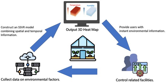
Figure 1.
Continuous Monitoring and Decision Process.
The main advantage of -SSVR model is the capability to adjust the objective -insensitive loss function based on real and synthetic sensors, where -insensitive loss function indicates that only the absolute error between the estimated and the observed values of an instance larger than value will be accounted for. Since the readings of synthetic sensors are interpolated, which may reflect higher measurement errors than those of real sensors, we give real sensors with smaller , while synthetic sensors with larger one.
2. Related Work
The related research topics for our experiment are divided into three categories: (1) coverage hole problem, (2) interpolation method for globally 3-D heat map, and (3) monitoring model.
The coverage hole problem is common for sensor deployment and is discussed in many studies of WSNs. To deal with such problem, we have to first define a coverage model for the sensor. Boudaren et al. [16] mentioned three kinds of coverage models. Deterministic coverage models classify a point to be either certainly within a specific region (i.e., covered by a sensor) or not. Probabilistic models represent the probability of a point being covered. The longer the distance between the point and the sensor, the less likely it is for the point to be covered. At last, Evidential sensing models are designed to handle the uncertainties by taking into account the reliability of the sensors. Note that the coverage models do not have to be in a circular shape. Some coverage hole problems are due to abnormalities in the values recovered by the sensors.
Since it is impossible to arrange full sensing points in space, and the sensors in most cases are sparse, the interpolation method becomes very important for those positions without sensors. The study of Li and Heap [17] divides the interpolation methods into three categories and briefly describes more than 40 spatial interpolation methods. They also discuss the factors that affect the performance [18]; there are a total of 25 classifications of common methods according to characteristics of the interpolation models. Finally, a decision tree that selects the appropriate method from these 25 methods is developed. The study of Bargaoui and Chebbi [19] uses a cross-validation scheme to compare the accuracy of two kriging methods (2-D, 3-D). The 3-D kriging method derived from the rainfall data leads to a significantly lower prediction error than the classic 2-D kriging method. In the study of Zhang et al. [20], rainfall data from the agro-ecological monitoring network was assessed, and four spatial interpolation methods were used to generate a map of the total monthly rainfall in Sri Lanka.
In regards to monitoring models, the study of Danielsen et al. [21] integrates various monitoring methods to monitor natural resources for the habitats of the species in order to assist conservation biologists in identifying and establishing monitoring systems that are most relevant to specific environmental protection. Hu et al. [22] use a support vector regression model to monitor air pollution and obtain results that are more accurate than those from artificial neural network models. Obviously, monitoring is widely used for different purposes. The research of Shen et al. [23] is related to our goal, which monitors the 2-D plane of greenhouse and has proposed a distributed anomaly detection mechanism to report the abnormal information. Based on the data from the greenhouse of the Martens Greenhouse Research Foundation in western Finland [7], it is possible to detect local differences caused by various disturbances in greenhouse climate. In our research, we are going to combine either spatial and/or temporal features to build a monitoring model and output continuous 3-D heat maps.
3. Coverage Hole Problem
3.1. Virtual Sensors via Uniform Design Sampling
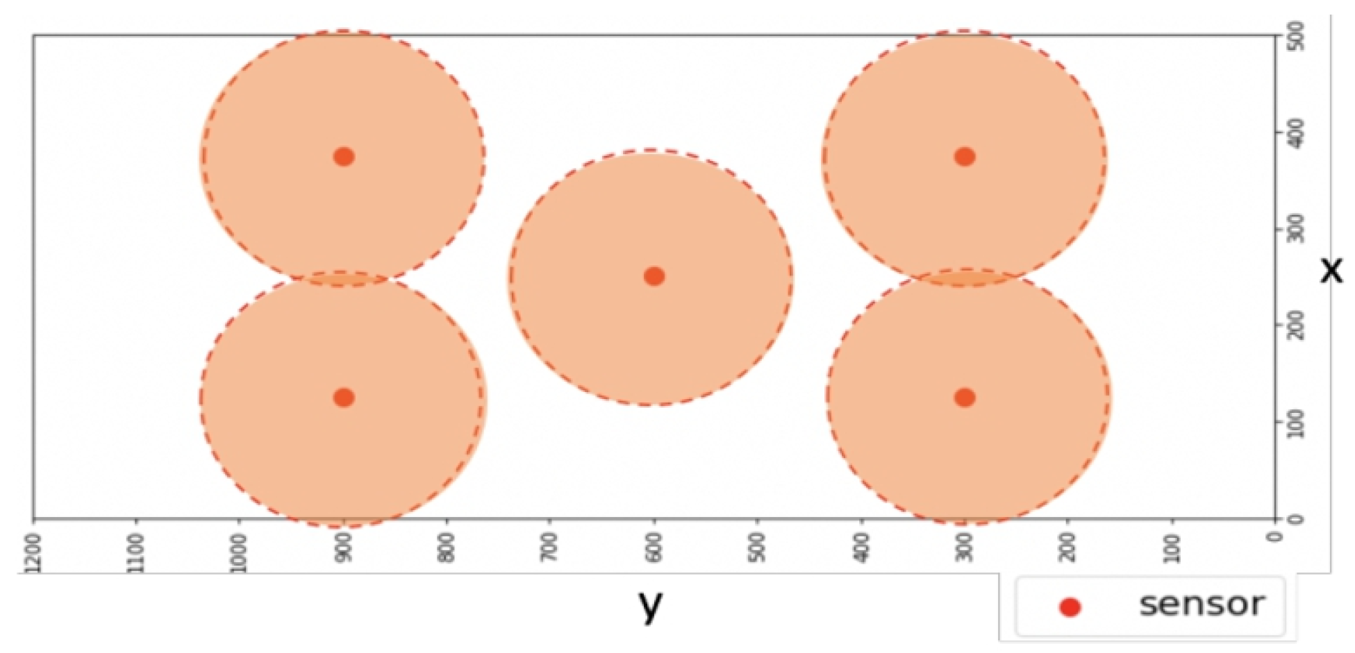
To solve the coverage hole problem (Figure 2), here we introduce a method called “uniform design (UD)” which is popular in the industrial experimental design [24]. In ANOVA-based experiment design model, there are s factors with q levels for each, resulting in a total of experimental combinations for testing the main and interaction effects among all factors. Obviously, the number of experiments increases exponentially with the number of factors as well as levels. Therefore, the objective is to utilize a few experiments instead of all while maintaining a good parameter estimation.

Figure 2.
Coverage Hole Problem. The orange circle is the sensing range of the sensor. It shows that the range of each sensor is limited, so it cannot cover the entire plane.
UD can effectively reduce the number of experiments (say, from to n) with better design flexibility and uniformity, which reduces time consumption effectively in industrial experiments and has a good estimate of nonlinear models [12]. The n experimental combination is symbolized as in the uniform design table referred to [25].
In our research, we use UD in the following two applications: (1) positioning of the synthetic sensors and (2) parameter tuning for our monitoring model (i.e., -SSVR) instead of the grid search.
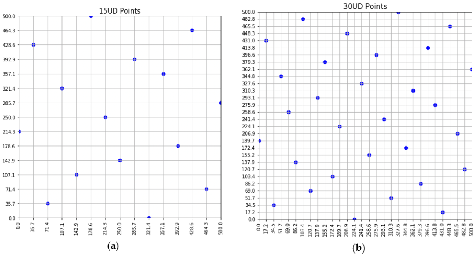
In application of positioning the synthetic sensors in 2-D space, the factors represent the length and width of the plane (i.e., ), and each factor has levels (hence we can position synthetic sensors on the plane). We then can refer to UD for the coordinate of each synthetic sensor. An illustration of all synthetic sensors is shown in Figure 3.
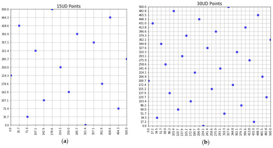
Figure 3.
Uniform design showing the positions of synthetic sensors with: (a) n = 15; (b) n = 30 points.
3.2. Interpolation Method
After positioning the synthetic sensors, the next important task is to estimate the readings of each sensor at any time point, which is an interpolation problem. The commonly used local linear models for interpolation are IDW and OK, which can be referred to [10,11,26,27]. By “local” it means only the nearest k neighboring sensor readings are used for calculation. In our experiment, we consistently set for all interpolation.
In addition, we notice empirically that the readings (e.g., temperature in our case) in the vertical direction change more drastically than those in the horizontal direction. More specifically, the temperature reading becomes higher along with greater height; while temperature readings from the same horizontal plane have subtle changes. This causes issues when using ordinary OK and IDW in our research domain, such as over-estimation for synthetic sensor values on smaller height (z-axis) and under-estimation on larger height, showing the unreasonable influence of z-axis. We thus develop a two-step new interpolation method, that is, the variants of IDW and OK (called zIDW and zOK).
Operationally, we treat the information from xy-plane differently from z-axis. More specifically, given any synthetic sensor point at position (), we first project it vertically to all non-redundant planes where real sensors locate (i.e., , , which means the number of non-redundant planes). We then locally interpolate each projected location in either by IDW or OK based solely on their horizontal real sensors and hence derive a vertical line of interpolated values along (). At last, we can apply these interpolations to again interpolate the target synthetic sensor at (, ) linearly or nonlinearly (according to the scatter of interpolations of ). Notice that if , only linear interpolation model can be used as the case in our experiment.
4. Monitoring Model via -SSVR
4.1. -Smooth Support Vector Regression Model
Let be a training dataset. In traditional ordinary regression, the objective is to find a hyperplane with the least-squared method so as to best fit the dataset S. SVR can be regarded as a generalization from ordinary regression, which adds a tolerance parameter to discard small errors when fitting the training points. As shown in Figure 4, the loss function of each instance given parameter can be written as:
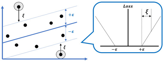
Figure 4.
-insensitive loss function.
That is, if the absolute discrepancy between predicted value and the observed value is less than a given value (i.e., ), then the loss value of such instance is regarded as 0.
The objective of linear SVR is to find a hyperplane of which the constrained minimization problem is generally formulated as follows:
In linear -SSVR [13,14], the above Equation (2) can be reformulated into an unconstrained minimization problem is as the following [13]:
Furthermore, to make the objective function twice differentiable, which can be quickly solved by Newton’s method, Lee et al. [13] used the smooth p-function (i.e., ) tuned by a smoothing parameter to replace the error term () of SVR (i.e., controls how much the error term be approximated by p-function). Thus, the minimization problem is then reformulated into the following (refer to [13] for more detail):
Notice that synthetic sensors have a larger tolerance values than that of real sensors in our experiment, which shows:
where and are the index sets of synthetic and real sensors, respectively, s. t. .
4.2. Nonlinear -Smooth Support Vector Regression
We can extend linear case to nonlinear case through the dual formulation of minimization problem [13]. In order to achieve this, we employ a kernel function which represents the dot product of two training points in a higher dimensional space. In general, there are many forms of kernels, and the Gaussian kernel (also known as radical basis function (RBF) kernel) is one of the commonly used as defined in Equation (6), which is also used in our experiment:
where is a tuning parameter determining how far the influence of squared Euclidean distances between the two feature vectors reaches.
4.3. Spatial and Temporal Features
Usually, the sensor information includes ID, location, measurement (i.e., temperature in our case), and timestamp. Thus, to predict the temperature at any unmeasured location at timestamp t (), we incorporate spatial (S) as well as temporal (T) features, and introduce four -SSVR related models.
For spatial model (SSVR (S)), features include 3-D sensor location (i.e., for each sensor case i), of which the training data is illustrated in Table 1 with, say, sensors at timestamp t. For temporal model (SSVR (T)), features include the past h values of temperature (i.e., )), of which the training data is illustrated in Table 2 with (which is also the value we set for temporal model in our experiment). In the same manner, the spatial and temporal model (SSVR (S&T)) includes aforementioned features (i.e., ), of which the training data can be formed by concatenating Table 1 and Table 2. Notice that if we incorporate synthetic sensors for model training, it follows the exact rationale. The only difference is that the training data size is expanded by containing cases of both real and synthetic sensors (e.g., with 10 real sensors and 30 synthetic sensors).

Table 1.
The form of training data for spatial model at timestamp t.

Table 2.
The form of training data for temporal model at timestamp t.
Beyond these models, we also combine SSVR (S) and SSVR (T) models to strengthen our prediction (named SSVR (S + T) for convenience); this is to deal with the scenario that, when the temperature has a sharp rise or falls along the time, the temporal model will be overestimated or underestimated. We then design the model as below:
where and represent the temperatures estimated by the spatial and temporal models, respectively, at timestamp t; is a weighting parameter ; is to limit the difference of temperatures from the spatial and temporal models. That is to say, if the difference is larger than , then we only consider the estimated values from spatial model; otherwise, we derive a weighted average. is thus the estimated temperature from a combination of the spatial and temporal models.
4.4. Architecture
The continuous monitoring architecture to build a globally 3-D heat map at any timestamp t is shown in Figure 5. There are two steps. The first step is to reduce the coverage hole problem due to sparsity of the sensor deployment. We thus apply UD to generate multiple synthetic sensors deployed in 3-D space, of which the readings are interpolated by local linear model (e.g, IDW, OK,…). The second step is then to apply the -SSVR models (as introduced previously) to fit the globally monitoring model by combining real and synthetic sensor readings. At last, the output is a consecutive 3-D heat map for any timestamp t.
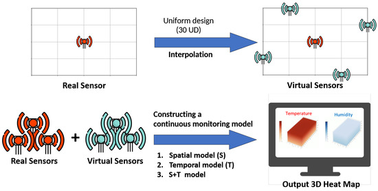
Figure 5.
Continuous Monitoring Architecture.
5. Experiments
5.1. Data Description
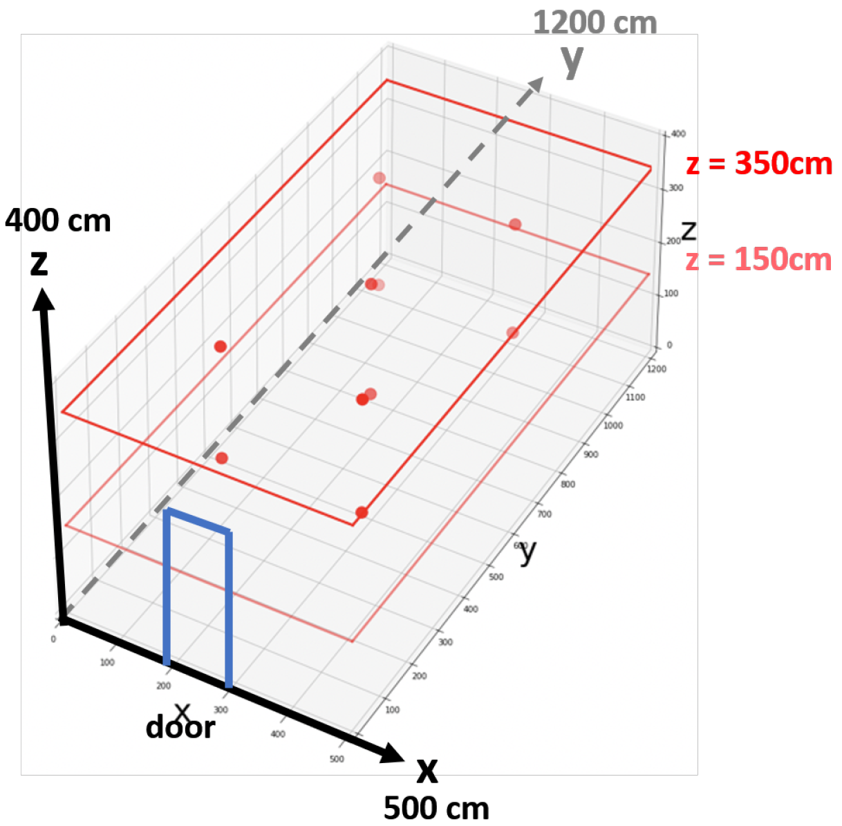
Our smart greenhouse field is in Wufeng District, Taichung—a rectangular parallelepiped with (length (X), width (Y), height (Z)) = (500, 1200, 400) (scale: cm), which could monitor the growth conditions of cherry tomatoes. In smart greenhouse, there are 2 horizontal layers (i.e., Loc.Z = 150 and 350 cm), each having 5 E-type thermometers deployed (red points in Figure 6. The frequency of each sensor data is one reading per ten minutes. The sensors are coded from 1 to 5 on Loc.Z = 150, and 6 to 10 on Loc.Z = 350. For either layer of Z, the corresponding (Loc.X, Loc.Y) = { (375, 300), (125, 300), (250, 600), (375, 900), (125, 900)}.

Figure 6.
Smart Green House Architecture.
5.2. Experimental Process and Parameter Tuning
We evaluate our nonlinearly extended models—SSVR(S), SSVR(T), SSVR(S&T), and SSVR(S+T) under the condition either with or without synthetic sensors, to compare the marginal effect of synthetic sensors; we also compare our method with OK and IDW as baseline models. To validate our methods, the leave-one-out (LOO) strategy is used to each of real sensors where we can calculate our error rate by comparing the actual value and the predicted value. More specifically, for i-th real sensor being tested () at time t, the training data would be composed of the rest of sensor information (either with or without synthetic sensors) at time t. We can thus estimate the values of i-th real sensor for any time t (). As a result, for each trial of real sensor, the evaluation metrics can be calculated by Mean Absolute Error (MAE) and Root Mean Square Error (RMSE):
where and represent the actual and predicted values of real sensor i at time t, respectively.
In regard to parameter tuning for each of our nonlinear models, we use the aforesaid LOO strategy on the whole sample, and the set of parameters with the lowest averaged MAE as well as averaged RMSE across all trials of real sensors is determined as the best solution (refer to Table 3). Except for SSVR (S&T) model, we incorporate 30 synthetic sensors by UD method (i.e., ) during parameter tuning process. The reason for SSVR (S&T) model will be explained at the latter section. Notice that the error tolerance of synthetic sensors is larger than that of the real sensors (), thus the parameter values tuned for the former are mostly larger than that of the latter (i.e., [0.1, 2] v.s. [0.01, 0.2]), and the results of mean and standard deviation (STD) of MAE and RMSE with the optimum parameter setting are displayed in the following section, which can be regarded as the best-case scenario for each model incorporating synthetic sensors.

Table 3.
Parameter setting.
6. Results
Our experimental results are presented in two ways: (i) numerical results and (ii) output of 3-D heat maps. The results of such experiments can indicate whether there is an improvement in model accuracy and a solution to the coverage hole problem.
6.1. Numerical Results
Table 4 shows the results under the existence of coverage hole problem (i.e., without synthetic sensors), which are derived from traditional spatial models such as IDW and OK, as well as regression-based nonlinear -SSVR models introduced previously. It can be found that the accuracy of the -SSVR models is better than that of traditional ones. Among -SSVR models, SSVR (S + T) has the best performance, while SSVR (T) the worst.

Table 4.
Results under the coverage hole setting (without synthetic sensors).
Next we show the results of adding synthetic sensors in Table 5. Notice that the SSVR(S&T) model is not included since it does not improve much from SSVR (S) and SSVR (T) models (thus there is no tuning parameter ). It is found that no matter which interpolation method (zIDW or zOK) we used, the accuracy was improved by reducing MAE and RMSE by about 0.03 to 0.3, indicating a good marginal effect of incorporating synthetic sensors. Again, SSVR(S + T) has the best performance (with zIDW + SSVR (S + T) slightly better than zOK + SSVR (S + T)), while SSVR (T) the worst.

Table 5.
Results with synthetic sensors.
In both conditions above, spatial information contributes more than temporal information, which uses only h = 3 past values as features. An interesting observation is that, after adding synthetic sensors, the STD of MAE and RMSE from SSVR(T) model increase significantly, whereas that from SSVR(S) decreases also significantly, although they all improve MAE and RMSE in average. That means the spatial interpolation methods diverge from the predictions of the temporal model (SSVR(T)) but narrow them down for the spatial model (SSVR(S)). Accordingly, it is suggested that an interpolation method using temporal clues be introduced for improving the temporal model.
6.2. Output of 3-D Heat Maps
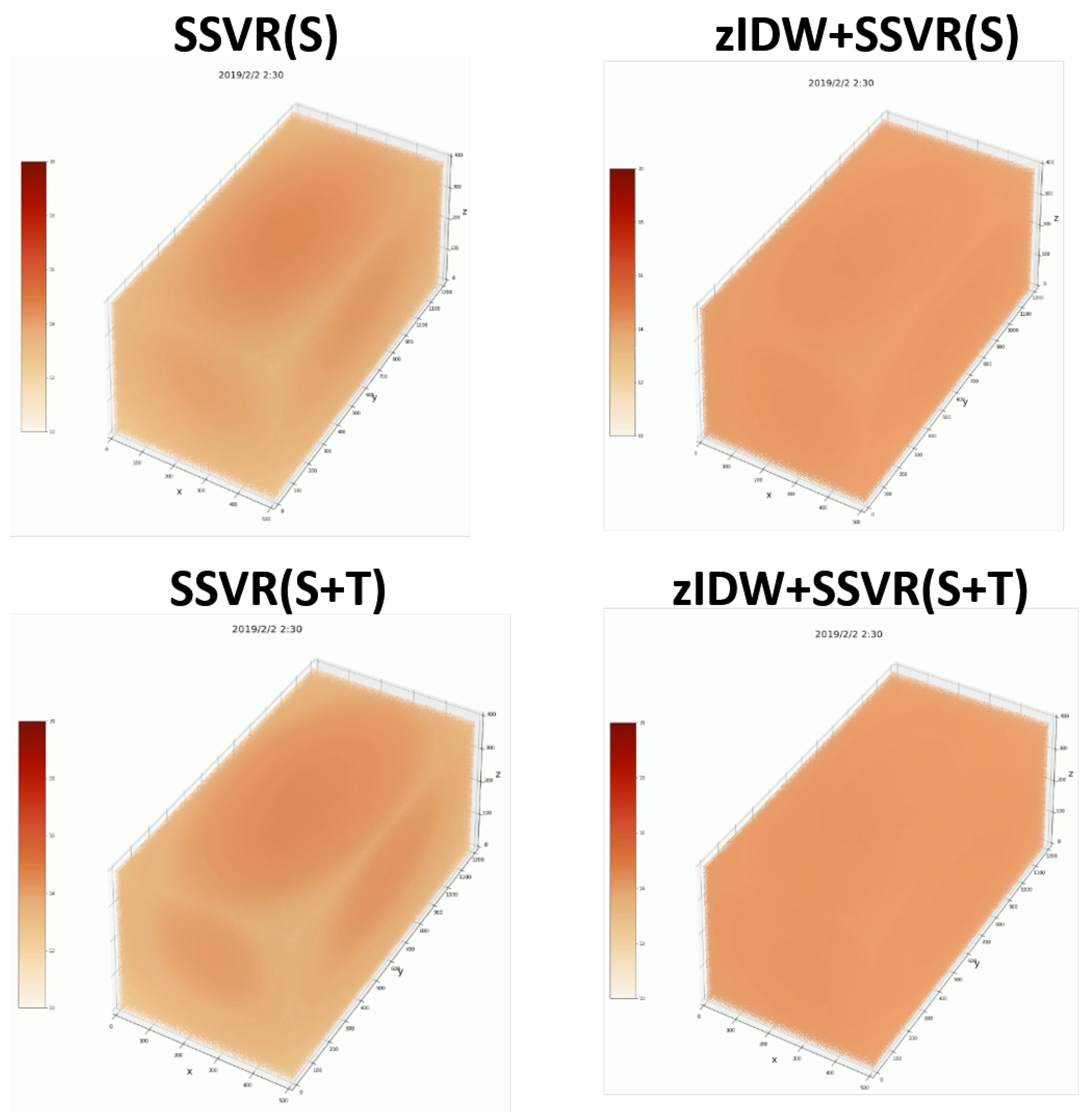
We also examine the results by heat maps. Here we compare the heat maps from four models—SSVR (S), SSVR (S + T), zIDW + SSVR (S), and zIDW + SSVR (S + T) illustrated in Figure 7. The lighter the color is, the lower the temperature becomes; and it is obvious for models without synthetic sensors (i.e., without zIDW interpolation) that they have mis-predicted values at the eight corners of the greenhouse (like a darker football crammed in a light-colored container), while models with synthetic sensors have less of such issues. On the whole, adding synthetic sensors improves model performance, and zIDW + SSVR (S + T) model has more realistic results than other models.

Figure 7.
Heat maps comparison with four continuous monitoring models of temperature.
7. Conclusions and Future Work
In this thesis, we can see from the experimental results that using the -SSVR model to construct a global monitoring model has better performance than the traditional interpolation method IDW and OK. Moreover, the coverage hole problem can be solved by incorporating synthetic sensors through the following procedure: (i) adding virtual points in space by using uniform design, (ii) applying interpolation method (e.g., zIDW or zOK in our case) for synthetic data generation, (iii) combining real and synthetic sensor data (spatial and temporal) for -SSVR model buildup. The above effectively improve the estimation accuracy of continuous monitoring model.
It is worth noting that in our experiment, spatial clues contribute more to the model performance than temporal clues of only past points. The possible suggestion is to add more past points (i.e., greater h) to the temporal model in future work. Furthermore, the interpolation method including temporal clues may also be considered to improve the quality of the data.
While the current model verification uses LOO strategy to each sensor, it is preferred, for the future experiment, to launch an automatic drone equipped with sensors to patrol the greenhouse field, from which the collected data (i.e., testing set) can be directed used for model validation. The drone can collect more thorough ambient data than those of the fixed-point sensors, thus providing more complete evaluation of the models.
In future applications, the 3-D monitoring model of ambient factors (e.g., temperature, humidity, etc.) can be integrated into the automated control system of the greenhouse; for heat management, as an instance, it is crucial when and where to open the widows or fans under current estimation of heat map. Furthermore, to improve the estimation of greenhouse environment, we can also combine the meteorological data from a local micro-weather station [28,29] such as wind speed, solar radiation [30], and so on. Other factors might include ambient conditions, for example, the state of ventilation equipment (windows or fans on or off ), endothermic processes from crop transpiration, and soil evaporation.
In addition, greenhouse environmental factors are mostly modeled and monitored by the computational fluid dynamics (CFD) field. However, in the modeling process of CFD, the setting of environmental parameters is often an important task. As a result, we can also apply -SSVR global monitoring model to help decide parameter values such as greenhouse transparency, air thermal conductivity and aerodynamic viscosity for the fluid mechanics.
Author Contributions
Conceptualization, Y.-J.L.; methodology, Y.-J.L., Y.-R.J., C.-Y.C., and Y.-H.Y.; software and formal analysis, Y.-R.J., C.-Y.C., and Y.-H.Y.; writing—original draft preparation, Y.-R.J.; writing—review and editing, H.-C.H.; supervision, Y.-J.L. and H.-C.H. All authors have read and agreed to the published version of the manuscript.
Funding
This research was funded by the Ministry of Science and Technology, via grant number MOST 107-2321-B-055-002.
Acknowledgments
We are very grateful to the Taiwan Agricultural Research Institute Council of Agriculture, Executive Yao for providing us with the experimental field in Taichung and helping considerably with setting up the sensor.
Conflicts of Interest
The authors declare no conflict of interest. The funders had no role in the design of the study; in the collection, analyses, or interpretation of data; in the writing of the manuscript; or in the decision to publish the results.
Abbreviations
The following abbreviations are used in this manuscript:
| -SSVR (or SSVR) | -Smooth Support Vector Regression |
| UD | Uniform Design |
| IDW | Inverse Distance Weighting |
| OK | Ordinary Kriging |
References
- Chong, C.Y.; Kumar, S.P. Sensor networks: Evolution, opportunities, and challenges. Proc. IEEE 2003, 91, 1247–1256. [Google Scholar] [CrossRef]
- Ramson, S.J.; Moni, D.J. Applications of wireless sensor networks—A survey. In Proceedings of the 2017 International Conference on Innovations in Electrical, Electronics, Instrumentation and Media Technology (ICEEIMT), Coimbatore, India, 3–4 February 2017; pp. 325–329. [Google Scholar] [CrossRef]
- Ko, J.; Lu, C.; Srivastava, M.B.; Stankovic, J.A.; Terzis, A.; Welsh, M. Wireless sensor networks for healthcare. Proc. IEEE 2010, 8, 1947–1960. [Google Scholar] [CrossRef]
- Römer, K.; Mattern, F. The design space of wireless sensor networks. IEEE Wirel. Commun. 2004, 11, 54–61. [Google Scholar] [CrossRef]
- Akyildiz, I.F.; Su, W.; Sankarasubramaniam, Y.; Cayirci, E. A survey on sensor networks. IEEE Commun. Mag. 2002, 40, 102–116. [Google Scholar] [CrossRef]
- Abbasi, A.Z.; Islam, N.; Shaikh, Z.A. A review of wireless sensors and networks’ applications in agriculture. Comput. Stand. Interfaces 2014, 36, 263–270. [Google Scholar] [CrossRef]
- Ahonen, T.; Virrankoski, R.; Elmusrati, M. Greenhouse Monitoring with Wireless Sensor Network. In Proceedings of the 2008 IEEE/ASME International Conference on Mechtronic and Embedded Systems and Applications, Beijing, China, 12–15 October 2008; pp. 403–408. [Google Scholar]
- Ahmed, N.; Kanhere, S.S.; Jha, S. The holes problem in wireless sensor networks: A survey. ACM SIGMOBILE Mob. Comput. Commun. Rev. 2005, 9, 4–8. [Google Scholar] [CrossRef]
- Wang, B.; Wang, W.; Srinivasan, V.; Chua, K.C. Information coverage for wireless sensor networks. IEEE Commun. Lett. 2005, 9, 967–969. [Google Scholar] [CrossRef]
- Zimmerman, D.; Pavlik, C.; Ruggles, A.; Armstrong, M.P. An Experimental Comparison of Ordinary and Universal Kriging and Inverse Distance Weighting. Math. Geol. 1999, 31, 375–390. [Google Scholar] [CrossRef]
- Caruso, C.; Quarta, F. Interpolation methods comparison. Comput. Math. Appl. 1998, 35, 109–126. [Google Scholar] [CrossRef]
- Fang, K.T.; Lin, D.K.; Winker, P.; Zhang, Y. Uniform Design: Theory and Application. Technometrics 2000, 42, 237–248. [Google Scholar] [CrossRef]
- Lee, Y.J.; Hsieh, W.F.; Huang, C.M. ε-ssvr: A smooth support vector machine for ε-insensitive regression. IEEE Trans. Knowl. Data Eng. 2005, 5, 678–685. [Google Scholar] [CrossRef]
- Gu, W.; Chen, W.P.; Ko, C.H.; Lee, Y.J.; Chen, J.S. Two smooth support vector machines for ε-insensitive regression. Comput. Optim. Appl. 2018, 70, 171–199. [Google Scholar] [CrossRef]
- Smola, A.J.; Schölkopf, B. A tutorial on support vector regression. Stat. Comput. 2004, 14, 199–222. [Google Scholar] [CrossRef]
- Boudaren, M.E.Y.; Senouci, M.R.; Senouci, M.A.; Mellouk, A. New trends in sensor coverage modeling and related techniques: A brief synthesis. In Proceedings of the 2014 International Conference on Smart Communications in Network Technologies (SaCoNeT), Vilanova i la Geltru, Spain, 18–20 June 2014; pp. 1–6. [Google Scholar]
- Li, J.; Heap, A.D. A Review of Spatial Interpolation Methods for Environmental Scientists; Geoscience Australia: Canberra, Australia, 2008; pp. 137–145.
- Li, J.; Heap, A.D. Spatial interpolation methods applied in the environmental sciences: A review. Environ. Model. Softw. 2014, 53, 173–189. [Google Scholar] [CrossRef]
- Bargaoui, Z.K.; Chebbi, A. Comparison of two kriging interpolation methods applied to spatiotemporal rainfall. J. Hydrol. 2009, 365, 56–73. [Google Scholar] [CrossRef]
- Zhang, R.P.; Jing, G.; Liang, T.G.; Feng, Q.S.; Aimaiti, Y. Comparing interpolation techniques for annual temperature mapping across Xinjiang region. IOP Conf. Ser. Earth Environ. Sci. 2016, 46, 1–6. [Google Scholar] [CrossRef]
- Danielsen, F.; Burgess, N.D.; Balmford, A.; Donald, P.F.; Funder, M.; Jones, J.P.; Alviola, P.; Balete, D.S.; Blomley, T.; Brashares, J.; et al. Local participation in natural resource monitoring: A characterization of approaches. Conserv. Biol. 2009, 23, 31–42. [Google Scholar] [CrossRef]
- Hu, K.; Sivaraman, V.; Bhrugubanda, H.; Kang, S.; Rahman, A. SVR based dense air pollution estimation model using static and wireless sensor network. IEEE Sens. 2016. [Google Scholar] [CrossRef]
- Shen, Y.C.; Chiang, A.; Yeh, Y.R.; Lee, Y.J. Continuous monitoring and distributed anomaly detection for ambient factors. In Proceedings of the 2014 IEEE International Conference on Internet of Things (iThings), and IEEE Green Computing and Communications (GreenCom) and IEEE Cyber, Physical and Social Computing (CPSCom), Taipei, Taiwan, 1–3 September 2014; pp. 31–38. [Google Scholar] [CrossRef]
- Huang, C.M.; Lee, Y.J.; Lin, D.K.; Huang, S.Y. Model selection for support vector machines via uniform design. Comput. Stat. Data Anal. 2007, 52, 335–346. [Google Scholar] [CrossRef]
- Hong Kong Baptist University. The Uniform Design. Available online: http://www.math.hkbu.edu.hk/UniformDesign/ (accessed on 2 October 2019).
- Oliver, M.A.; Webster, R. A tutorial guide to geostatistics: Computing and modelling variograms and kriging. Catena 2014, 113, 56–69. [Google Scholar] [CrossRef]
- Chiles, J.P.; Delfiner, P. Geostatistics: Modeling Spatial Uncertainty, 2nd ed.; John Wiley & Sons: Hoboken, NJ, USA, 2012; ISBN 978-047-018-315-1. [Google Scholar]
- Zhang, Y.; Hamm, N.A.; Meratnia, N.; Stein, A.; Van De Voort, M.; Havinga, P.J. Statistics-based outlier detection for wireless sensor networks. Int. J. Geogr. Inf. Sci. 2012, 26, 1373–1392. [Google Scholar] [CrossRef]
- Liu, C.Y.; Chuang, C.L.; Chen, C.P.; Chang, W.Y.; Shieh, J.C.; Lin, C.H.; Tseng, C.L.; Jiang, J.A. Development of an embedded system-based gateway for environmental monitoring using wireless sensor network technology. In Proceedings of the 2011 Fifth International Conference on Sensing Technology (ICST), Palmerston North, New Zealand, 28 November–1 December 2011; pp. 544–548. [Google Scholar] [CrossRef]
- Mesmoudi, K.; Soudani, A.; Bournet, P.E. Determination of the inside air temperature of a greenhouse with tomato crop under hot and arid climates. J. Appl. Sci. Environ. Manag. 2010, 5, 117–129. [Google Scholar]
© 2019 by the authors. Licensee MDPI, Basel, Switzerland. This article is an open access article distributed under the terms and conditions of the Creative Commons Attribution (CC BY) license (http://creativecommons.org/licenses/by/4.0/).


