On ADS-B Sensor Placement for Secure Wide-Area Multilateration ^†

Abstract

As automatic dependent surveillance–broadcast (ADS-B) becomes more prevalent, the placement of on-ground sensors is vital for Air Traffic Control (ATC) to control the airspace. However, the current sensors are placed in an unstructured way that keeps some areas without coverage, and others are over-densified by sensors. Therefore, areas with coverage anomalies may cause issues that inhibit accurate ADS-B verifications as well as the availability of ADS-B altogether. In this paper, we tackle the ADS-B-specific optimal sensor placement (OSP) problem. Of importance are both the optimal coverage and the secure and accurate verification of received ADS-B messages. Specifically, we take into account the following objectives. First, we determine the minimum required number of sensors in order to cover a certain area like Europe. Second, we produce a better placement of the current sensors with respect to the security and accuracy of geometric dilution of precision (GDOP). Finally, we calculate how far the current sensor setup is from our derived optimal solution as well as the cost to reach the optimality. Our experiments show that the ideal fitness score for solving the OSP is below 0.1, meaning that the mean squared error (MSE) of the required and achieved GDOPs is significantly small, thus accomplishing a near-optimal setup.

1. Introduction

As of the year 2020, most commercial aircraft have been equipped with an automatic dependent surveillance–broadcast (ADS-B) transponder to comply with the DO-260B mandate. In parallel with this ongoing upgrade of airplanes, low-cost ADS-B receivers on the ground are being deployed for air-traffic monitoring. As aircraft follow normal routes, placing the ADS-B ground sensors in specific locations may not turn out to be cost effective, as the ground sensors may never receive the broadcast signals. Moreover, an over-densification of receivers in the same area does not necessarily improve the deployment gain in terms of coverage and does not facilitate the application of data fusion or multilateration-based mechanisms. Wide-area multilateration (WAM) based on Time Difference Of Arrival (TDOA) measurements is one of the preferred methods for verifying the accuracy and integrity of ADS-B position reports [1,2]. This is, however, only possible if the target aircraft is visible from at least four ground-based receivers.

This paper tackles the optimal sensor placement (OSP) problem for the multi-objective deployment of ADS-B receivers on the ground. Of importance are both ① the optimal coverage and ② the secure and accurate verification of aircraft position information contained within ADS-B Out messages, that is, finding the placement of the receivers so that the position of the aircraft can be derived with an optimal accuracy.

The OpenSky network is one of most popular networks of ADS-B receivers, consisting of a large number of connected sensors that collect real-time traffic from ADS-B-based aircraft. Therefore, finding the proper placement of the ADS-B receivers so that each broadcasted ADS-B message could be received by a sufficient number of receivers on the ground is important. In our paper, we specifically target the deployment of OpenSky-based ADS-B sensors.

Problem Statement

Traffic from the OpenSky network reflects that there are geographic areas without ADS-B coverage and other areas that are over-densified by sensors. This situation makes flights more susceptible to attackers, as they can exploit the missing ADS-B availability and accuracy in order to carry out low-cost attacks on aircraft.

In this paper, we aim to:

• Find the minimal number of ADS-B receivers and their corresponding placement locations such that the entire airspace is optimally covered (no placement constraints).
• Find the best locations for placing n new sensors (without placement constraints) with respect to the existing deployed sensors.
• Choose the best n sensors from a set of existing proposed sensor locations (that are placed by volunteers who announce their interest in participation with their sensors) that gets the minimum geometric dilution of precision (GDOP) value.

2. Preliminaries

The approach we propose for tackling the OSP problem is based on the air-to-ground ADS-B signal propagation model, the time-of-arrival (ToA) localization technique, and sensor network design optimality criteria—more precisely, A-optimality [3]. We briefly introduce them in the following.

2.1. Air-to-Ground ADS-B Signal Propagation

For an ADS-B message transmitted by an aircraft to be successfully received by a ground sensor, a line-of-sight (LOS) condition must be met. The radio wave from transponders is radiated with sufficient power so that it is safe to assume that the maximum message reception range $r_0$ corresponds to the radio horizon [4]. Under tropospheric refraction, $r_0$ is given in kilometers by [5]:

$$r_0=3.57\sqrt{{\mathit{k}}_e}(\sqrt{h_1}+\sqrt{h_2}),$$

(1)

where ${\mathit{k}}_e$ represents the effective Earth-radius factor and $h_1$ (or $h_2$) represents the transmitter (or receiver) antenna height in meters. It follows that a sensor located beyond the instantaneous radio horizon of a given aircraft’s transponder will never receive an ADS-B signal radiated by the latter. In this case, the sensor is said to be deployed or situated out of reach of the aircraft.

2.2. Time-of-Arrival Localization

We consider the single aircraft emitter location estimation problem from ToA measurements using four distributed ADS-B sensors deployed at locations ${\mathbf{s}}_{\mathbf{i}}={[x_i,y_i,z_i]}^T,i=1,\dots ,4$. If the unknown true emitter location is denoted by $\mathbf{p}={[x,y,z]}^T$, the ToA measurement $t_i$ at the i-th sensor is given by [6]:

$$t_i=\frac{1}{c}\parallel \mathbf{p}-{\mathbf{s}}_{\mathbf{i}}\parallel +\tau +e_i,$$

(2)

where $\tau$ is the signal emission time, c is the speed of light, and $e_i$ is the measurement error. An estimate of $\mathbf{p}$ can be derived from Formula (2) by solving the system obtained from three ToA differences. The accuracy of this location estimation is affected by both the ranging errors and the geometric configuration of the sensors.

2.3. GDOP

Placing localization sensors too close to one another will degrade the GDOP and subsequently result in a high error for the estimated position. The GDOP is defined as [7]:

$$GDOP=\sqrt{tr{\left(B^{T}B\right)}^{-1}},$$

(3)

where

$$B={\left\{[b_{i1},b_{i2},b_{i3},1]\right\}}_{i=1,\cdots ,4},$$

(4)

and $b_{i1},b_{i2},$ and $b_{i3}$ are the direction cosines from the aircraft to the i-th sensor. We derive the matrix B defined in Equation (4) for computing the GDOP that would result when estimating the position of an aircraft located at $\mathbf{p}={[x,y,z]}^T$ from pseudo-range measurements taken at four sensors ${\mathbf{s}}_{\mathbf{i}}={[x_i,y_i,z_i]}^T$ in the Earth-centered, Earth-fixed (ECEF) coordinate system [8]. The GDOP at location $\mathbf{p}$ can subsequently be computed from Equation (3) using the closed-form expression derived in [7].

2.4. Sensor Deployment Optimality Criteria

There are three well-known optimality criteria for assessing the relative geometric configuration of a static or moving target with respect to a set of deployed sensors [3,9]. These are the A-, D-, and E-optimality, which utilize the Cramer–Rao Lower Bound (CRLB). The CRLB is generally used to give a lower estimate for the variance of an unbiased estimator. In this paper, we adopt the A-optimality metric for the ADS-B sensor placement where the mean squared error (MSE) on the location estimate is minimized through minimization of the trace of the CRLB. This is equivalent to minimizing the GDOP.

2.5. Genetic Algorithm (GA)

A genetic algorithm (GA) is a metaheuristic for solving (un-)constrained global optimization problems. The GA begins with a candidate population of individuals and repeatedly alters it through mutation and recombination of a subset of the current individuals to create a new population of offspring fitter than their parents. The population size remains constant across all generations, and the algorithm terminates when either the fitness of the best individual stops improving or a considerable number of generations has been examined. Regrading the OSP problem, we adapt the algorithm accordingly in the following sections.

3. Methodology

Our system model is designed to solve the OSP problem based on evaluating the GDOP principle in an attempt to provide full coverage; each air point in space is covered by at least four sensors on the ground, which is also to increase the Multilateration (MLAT) accuracy by reducing the GDOP values. In this paper, we tackle the OSP for a geographical area without coverage, meaning that there are no sensor placements, and a geographical area with existing sensors but at suboptimal placement.

3.1. Assumptions

For finding the optimal placement locations of sensors, we make the following simplifying assumptions:

• Receivers are assumed to be deployed on the geoid surface.
• We neglect the obstructing effect of buildings or mountains on the ADS-B signal reception probability.
• We consider the Earth’s curvature as the major impediment to the direct visibility between aircraft and ground-based sensors.

3.2. GDOP Evaluation Principle and Our Objective Function

Given an airspace volume $\mathcal{A}$ containing the expected source of ADS-B traffic, we systematically take m sample locations ${\mathbf{p}}_{\mathbf{j}}$ from $\mathcal{A}$ and define the following spatial data matrix:

$$\mathbf{A}={\left\{g_j\right|{\mathbf{p}}_{\mathbf{j}}\}}_{j=1,\cdots ,m},$$

(5)

where $g_j$ represents the required GDOP value at ${\mathbf{p}}_{\mathbf{j}}$. In addition, given a placement $\mathbf{S}={\left\{{\mathbf{s}}_{\mathbf{i}}\right\}}_{i=1,\cdots ,n}$ of n ADS-B sensors, we write $\widehat{g_j}=gdo{p}_{\mathbf{S}4pt}\left({\mathbf{p}}_{\mathbf{j}}\right)$ to denote the achieved GDOP value at the location ${\mathbf{p}}_{\mathbf{j}}$ due to the particular geometry of $\mathbf{S}$. For readability, we omit the subscript and note $\widehat{g_j}=gdop\left({\mathbf{p}}_{\mathbf{j}}\right)$.

Now, to find the minimal number of ADS-B sensors $n_{min}$ and their corresponding deployment $\mathbf{S}$ to guarantee a per-location GDOP requirement for a given airspace $\mathcal{A}$, let us assume $\delta$ to be the tolerance parameter on the GDOP at any location. A sensor placement $\mathbf{S}$ can only be admitted if:

$$\forall {\mathbf{p}}_{\mathbf{j}}\in \mathcal{A},|\widehat{g_j}-g_j|<\delta ,$$

(6)

which is equivalent to:

$${\parallel \widehat{\mathbf{g}}-\mathbf{g}\parallel }_{\infty }<\delta ,$$

(7)

where ${\parallel .\parallel }_{\infty }$ represents the sup-norm defined by:

$${\parallel \widehat{\mathbf{g}}-\mathbf{g}\parallel }_{\infty }=\underset{j}{max}|\widehat{g_j}-g_j|.$$

(8)

The mean squared deviation (MSD) between the achieved and the required GDOP in the entire airspace under consideration is written as:

$$MSD\left(\mathbf{S}\right)=\frac{1}{m}\sum _{j=1}^m{(g_j-\widehat{g_j})}^2.$$

(9)

3.3. System Approach

To solve the OSP problems, we adopt the MSD function to get the minimum GDOP for each air point based on the sensor placement setup. More specifically, for each transmitter location ${\mathbf{p}}_{\mathbf{j}}={[x_j,y_j,z_j]}^T$ in the ECEF frame, the corresponding geodetic coordinates are denoted as ${[{\lambda }_j,{\varphi }_j,h_j]}^T$. Let ${\mathbf{p}}_{\mathbf{j}}^{\prime }$ be the point on the geoid surface that has the same longitude and latitude as ${\mathbf{p}}_{\mathbf{j}}$. Assuming a ground-based deployment of receivers (i.e., each has an altitude of less than 10 m), it follows from Equation (1) that a sensor ${\mathbf{s}}_{\mathbf{i}}$ is in direct visibility with an emitter located at ${\mathbf{p}}_{\mathbf{j}}$ if and only if the following inequality is satisfied:

$$h_j\ge 0.0785\frac{{\parallel {\mathbf{p}}_{\mathbf{j}}^{\prime }-{\mathbf{s}}_{\mathbf{i}}\parallel }^2}{{\mathit{k}}_e}.$$

(10)

The achieved GDOP value $\widehat{g_j}=gdop\left({\mathbf{p}}_{\mathbf{j}}\right)$ is computed and evaluated as follows:

Find the set ${\mathcal{S}}_{LOS4pt}^j$ of all ADS-B receivers for which Inequality (10) is valid.

If $|{\mathcal{S}}_{LOS4pt}^j|<4$, set $\widehat{g_j}=\infty$ (the GDOP cannot be evaluated if there are less than four sensors in LOS condition with the aircraft).

Otherwise, compute the GDOP at ${\mathbf{p}}_{\mathbf{j}}$ for all four-sized subsets of ${\mathcal{S}}_{LOS4pt}^j$ using the closed-form expression proved in [7]. Then set $\widehat{g_j}$ to the minimal value found.

4. OSP Problems

We define three possible scenarios that we could face while trying to find the GDOP-optimal deployment solution. In the first scenario, we assume that we do not have any placed ground-sensors covering the airspace volume under consideration and thus, we are interested in finding the optimal solution to place n available sensors. In the second scenario, we build on the already placed sensors on ground and aim to find the smallest number and best locations of new sensors to place for getting optimal coverage. In the third scenario, we try to find the minimum number of sensors from n available sensors with pre-determined locations to satisfy the desired optimization problem requirements.

4.1. Scenario #1: OSP from Scratch

We consider an airspace volume $\mathcal{A}$, uncovered by any ADS-B receiver, and its derived spatial data matrix $\mathbf{A}$ as defined in (5). That is, each of the m systematically sampled locations ${\mathbf{p}}_{\mathbf{j}}$ in $\mathcal{A}$ has been assigned a required GDOP value $g_j$ to meet the WAM-based ADS-B message verification’s accuracy requirements. We wish to optimally (from a secure localization perspective) cover $\mathcal{A}$ with a budget of n sensors. This is equivalent to finding the optimal placement of the n available sensors that minimizes the overall GDOP deviation from the required values. The problem to solve is expressed as follows:

$${\mathbf{S}}^{*}=\underset{\mathbf{S}}{arg\; min}\left(\frac{1}{m}·{\parallel \widehat{\mathbf{g}}-\mathbf{g}\parallel }_2\right).$$

(11)

4.2. Scenario #2: Optimal Network Augmentation

In this scenario, we consider an existing network consisting of n ADS-B sensors deployed at known locations ${\mathbf{S}}^{\mathbf{depl}}={\left\{{\mathbf{s}}_{\mathbf{i}}\right\}}_{i=1,\cdots ,n}$. We assume that the GDOP for the MLAT-based ADS-B message verification does not meet the network-wide requirement. This may be the case, for example, if $n<n^{*}$ or $n\ge n^{*}$, but the existing deployment is sub-optimal. Suppose that l new sensors ${\mathbf{S}}^{\mathbf{new}}={\left\{{\mathbf{s}}_{\mathbf{i}}\right\}}_{i=n+1,\cdots ,n+l}$ must be deployed. We write:

$$\mathbf{S}=\left\{{\mathbf{S}}^{\mathbf{depl}},{\mathbf{S}}^{\mathbf{new}}\right\}={\left\{{\mathbf{s}}_{\mathbf{i}}\right\}}_{i=1,\cdots ,n+l}.$$

(12)

If we allow a subset of the sensors to have fixed predefined locations, then the OSP formulation expressed in (11) holds for the optimal network augmentation problem. ${\mathbf{S}}^{\mathbf{new}}$ must be chosen from a predefined set of candidate locations ${\mathbf{S}}^{\mathbf{cand}}={\left\{{\mathbf{s}}_{\mathbf{j}}^{\prime }\right\}}_{j=1,\cdots ,N}$. The aim in this particular case is to extend a preexisting network of $n=|S^{depl}|$ deployed sensors by selecting the best l of N possible locations.

4.3. Scenario #3: Best Sensors to Guarantee a Surveillance Requirement

The entire airspace may not be MLAT capable. This is because MLAT necessitates at least a network-wide four-coverage for a ubiquitous 3D emitter location estimation. In this scenario, we aim to find the best sensors $n_{min}$ among those proposed by volunteers to add to the existing sensor placement to guarantee a per-location GDOP requirement for a given airspace. A naive approach to finding the minimal number $n_{min}$ of sensors with optimal deployment that guarantees a lower bound of the WAM accuracy would be to use the well-known interval halving method or dichotomy, that is, to start the search with an initially high number of sensors $N_u$ that satisfies (6) and to repeatedly halve $N_u$ until a value $N_l$ is reached for which (6) cannot be met no matter the configuration of the receivers. The dichotomy can subsequently be used to find a good approximation of $n_{min}$ in the interval $[N_l,N_u]$.

5. Solving the OSP Problems

To explain our approach for solving OSP problems, we focus on solving the more general case, which is scenario #1 in this section. As an optimization technique to be adopted in this paper, we make use of a genetic algorithm (GA). In the sections below, we cover only the custom parts of the genetic algorithm that we altered in order to adapt it to the OSP problem appropriately.

5.1. Sensor Representation (Chromosomal Representation)

Under the assumption that sensors are deployed on the geoid surface, a candidate placement location is fully specified by its geodetic longitude and latitude. For the representation of each potential solution $\mathbf{S}={\left\{{\mathbf{s}}_{\mathbf{i}}\right\}}_{i=1,\cdots ,n}$ to the OSP problem to be unique, we consider the sensors in $\mathbf{S}$ to be sorted by increasing order of longitude. In case two sensors have identical longitudes, the one with the lower latitude is assigned the smaller index. We write:

$$\mathbf{S}=[({\theta }_1,{\mu }_1),\cdots ,({\theta }_n,{\mu }_n)],$$

(13)

where ${\theta }_i$ and ${\mu }_i$ are the longitude and latitude of the i-th sensor, respectively.

$${\forall }_{i=1}^{n-1},\left\{\begin{array}{c}{\theta }_i\le {\theta }_{i+1}\mathrm{and}\hfill \\ \mathrm{if}{\theta }_i={\theta }_{i+1}\mathrm{then}{\mu }_i\le {\mu }_{i+1}\hfill \end{array}\right.$$

(14)

Furthermore, the boundaries of the region in which sensors can be placed induce the following additional constraints:

$${\forall }_{i=1}^n,\left\{\begin{array}{c}{\theta }_l\le {\theta }_i\le {\theta }_u\hfill \\ {\mu }_l\le {\mu }_i\le {\mu }_u,\hfill \end{array}\right.$$

(15)

where ${\theta }_l$ (or ${\mu }_l$) and ${\theta }_u$ (or ${\mu }_u$) are the lower and upper bounds on each sensor longitude (or latitude).

5.2. Fitness Function

We adapt the fitness function according to the OSP problem using the MSD mentioned in Section 3.2 to calculate the fitness of an individual $\mathbf{S}$. It is used to evaluate each sensor placement in the population based on the MSD.

As an addition, we bolster our accuracy by defining a penalty or cost function and searching for the Pareto frontier [10] of the MLAT accuracy versus the cardinality of the sensor set. By discretizing the deployment area into a 2D grid of L rectangles where each can either be assigned a sensor ($w_i=1$) or not ($w_i=0$), a Knapsack-equivalent formulation of this problem would be to select as few rectangles as possible that are to be assigned a sensor while minimizing the network-wide GDOP. We define the following penalty or cost function h on the number of sensors deployed:

$$h\left(\mathbf{S}\right)=\frac{1}{2}·{\left[\frac{1}{L}\sum _{i=1}^L{w}_i\right]}^2.$$

(16)

Eventually, the weighted fitness function can subsequently be obtained from (9) and (16) as:

$$\tilde{f}\left(\mathbf{S}\right)=(1-a)·f\left(\mathbf{S}\right)+a·h\left(\mathbf{S}\right),$$

(17)

where a is the Pareto weight of the cost function h. A final fitness value below $0.1$ indicates a robust sub-optimal sensor placement, since the genetic algorithm converges to the local minimum(s) that significantly approximate the optimal setup (global minimum).

5.3. Selection Operation

The selection of the fittest individuals relies on the principles of natural selection. To be more specific, at each round or generation of the algorithm, individuals are ranked according to their fitness scores. Then, a subset of the best and random individuals is selected for the next round. Parents are chosen from this subset.

6. Experimental Evaluation

6.1. First Findings and Observations (“Random Sensor Placement”)

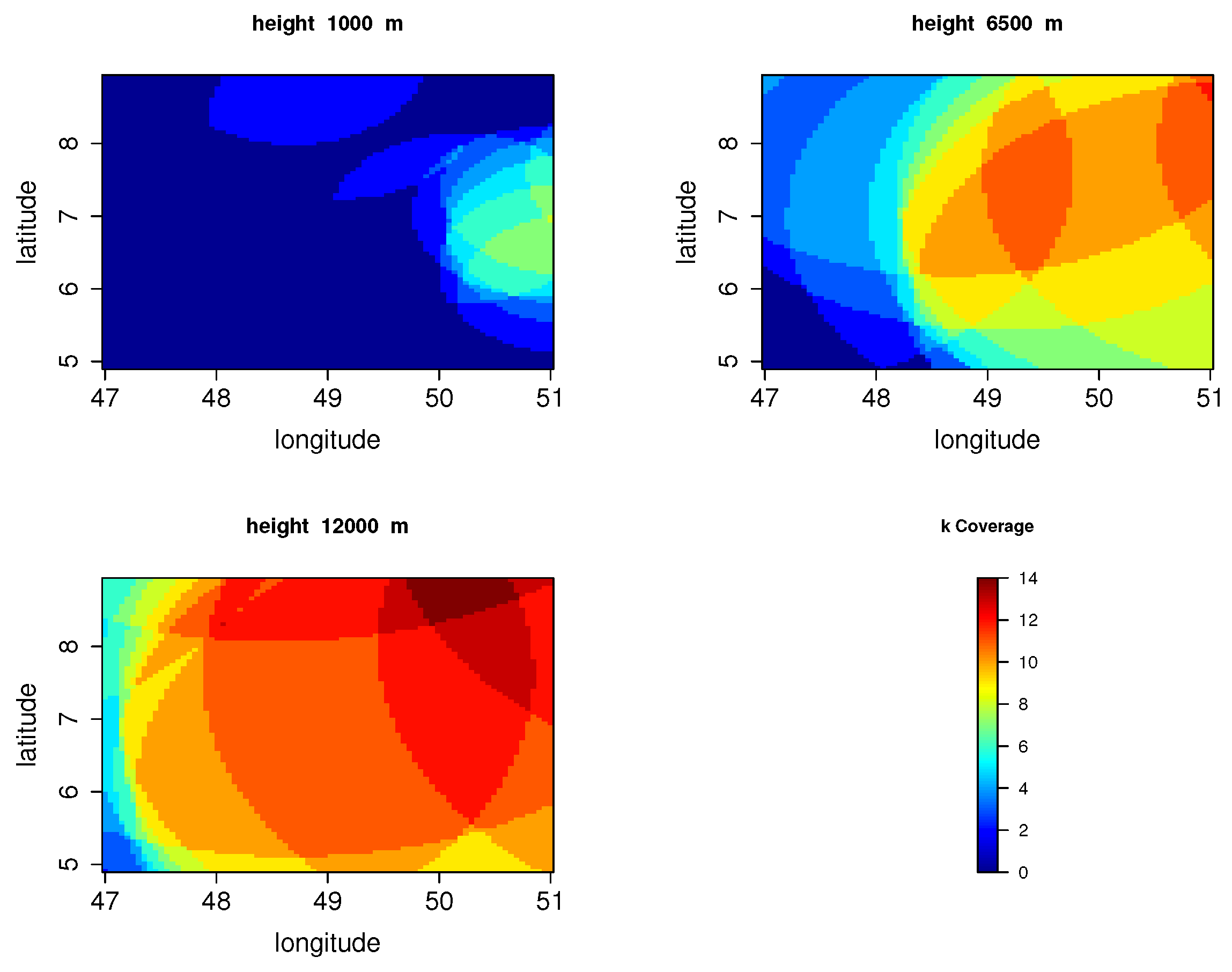
In this section, we illustrate the importance of an optimal deployment of WAM sensors by comparing the gain in the deployment quality metrics. Figure 1 shows the simulated k-coverage (an airspace location is said to be k-covered if an ADS-B-Out signal sourced from that location is received by exactly k ground sensors) at three different altitudes (1000, 6500, and 12,000 m) for a real-world random placement of $n=30$ receivers in a bounded geographic area spanning between the latitudes 4.9 and 8.9 decimal degrees and the longitudes 47 and 51 decimal degrees. The fitness score of this placement obtained by the simulation is 0.355, and the GDOP distribution in the airspace volume considered is illustrated in Figure 2. This placement is clearly sub-optimal because of the over-densification of the receivers in certain areas. At 1000 m altitude, some 3D locations are eight-covered, whereas others are covered by less than four sensors.

6.2. Achieved Results (Receiver Cardinality and Achievable Network-Wide GDOP)

For experimental evaluation, we consider a relatively small geographical area around Frankfurt airport with latitudes and longitudes ranging from 49 to 51 and from 7.5 to 9.5 decimal degrees, respectively. We used the genetic algorithm to find the best possible setup of sensors for all three scenarios. Furthermore, we parametrized the algorithm with 20 generations, 50 individuals (population size), Pareto weight equal to 0.8, and local search for optimization, while the probability parameters remained with their default values. In the first case, we were able to achieve a final placement with a fitness value equal to 0.0073 by utilizing only ten sensors. Figure 3 and Figure 4 show the significant reduction of the GDOP and high coverage of this placement. Finally, for the second scenario, we generated a sensor placement with a fitness score of 0.0037, and in the third scenario, we generated a fitness score of 0.218.

The algorithm searches for the best local minimums (near-optimal solutions) possible. Therefore, for the first case in Figure 5, it is able to reach the best local minimum after ten generations, since the placement starts from scratch. On the other hand, the algorithm is able to find the best possible solution for cases two and three immediately, as seen in Figure 6 and Figure 7, since there is already an existing (but not optimal) setup and a limited number of options. Kindly note that the minus notation in front of the fitness value is used only to instruct the algorithm to search for local minimums and not as a negative value (the fitness values are always non-negative numbers in our approach).

7. Related Work

In an unplanned ADS-B receiver network, the percentage of messages verifiable through WAM can be as low as 5.24% [11], that is, unless an alternative aircraft reports that a truthfulness verification technique such as k-NN is used, most of the messages remain vulnerable to spoofing attacks. WAM is nevertheless well known to provide a better median aircraft location error [11]. This justifies the importance of a security-aware ADS-B sensor placement.

The OSP problem in the avionic context has recently been investigated in [1]. Based on the assumption that MLAT applied with coplanar sensors generally results in a poor vertical dilution of precision, the authors disregard the aircraft height validation requirement and address the sensor placement for accurate latitude and longitude verification. More precisely, they minimize the expected horizontal error computed as the ratio between the common intersection area between all k-receiving sensors (also known as the k-coverage or k-intersection area) and the cumulative area covered by those sensors. This metric is, however, inaccurate, as a target location estimate error would be considered the same independently of its specific position within the k-covered area. We believe that if the MLAT sensors are carefully chosen and well spread, the Earth’s curvature can break the coplanarity assumption and, therefore, the GDOP is a more suitable figure of merit when judging the quality of an ADS-B receiver deployment.

The complementary problem of optimal sensor selection during the online aircraft tracking phase is addressed in [2]. This presupposes that (a) the existing sensor network infrastructure was thoughtfully deployed and (b) if the sensors are properly chosen, an acceptable end-to-end GDOP value can be attained. In fact, for static sensors, the existing deployment defines the lower bound on the achievable GDOP through an optimal MLAT sensor allocation.

In [12], the updated Fischer information matrix is used an as optimality criterion for an optimal non-static sensor motion coordination in real time for target tracking.

8. Conclusions

An optimal sensor placement (OSP) problem for the multi-objective deployment of ADS-B receivers on the ground is tackled by this paper. The proposed solution is based on the air-to-ground ADS-B signal propagation model, the time of arrival (ToA) localization technique, and sensor network design optimality criteria. We showed that it is possible to get a near-optimal setup of sensors that has minimum GDOP and large coverage, thus having a deployment that is more secure and more resilient to estimation errors.