Abstract
Unmanned aerial vehicles offer a safe and fast approach to the production of three-dimensional spatial data on the surrounding space. In this article, we present a low-cost SLAM-based drone for creating exploration maps of building interiors. The focus is on emergency response mapping in inaccessible or potentially dangerous places. For this purpose, we used a quadcopter microdrone equipped with six laser rangefinders (1D scanners) and an optical sensor for mapping and positioning. The employed SLAM is designed to map indoor spaces with planar structures through graph optimization. It performs loop-closure detection and correction to recognize previously visited places, and to correct the accumulated drift over time. The proposed methodology was validated for several indoor environments. We investigated the performance of our drone against a multilayer LiDAR-carrying macrodrone, a vision-aided navigation helmet, and ground truth obtained with a terrestrial laser scanner. The experimental results indicate that our SLAM system is capable of creating quality exploration maps of small indoor spaces, and handling the loop-closure problem. The accumulated drift without loop closure was on average 1.1% (0.35 m) over a 31-m-long acquisition trajectory. Moreover, the comparison results demonstrated that our flying microdrone provided a comparable performance to the multilayer LiDAR-based macrodrone, given the low deviation between the point clouds built by both drones. Approximately 85 % of the cloud-to-cloud distances were less than 10 cm.
Keywords:
drone; UAV; micro robot; loop closure; obstacle avoidance; mobile mapping; laser scanner; LiDAR; IMU; splines; 6DOF 1. Introduction
The provision of up-to-date information about indoor-environment layouts is vital for a wide range of applications, such as indoor navigation and positioning, efficient and safer emergency responses in disaster management and facility management. However, this study focuses on the disaster management application [1,2] as it is part of the Horizon 2020 project INGENIOUS [3] that aims to assist first responders to be more effective and make their jobs safer following natural and manmade disaster events.
Although many buildings have as-built 2D floor plans, these plans are usually not available quickly enough when needed. The plans are also often outdated because buildings change frequently, and it is costly to update their information using static mapping systems, such as terrestrial laser scanners (TLSs). Moreover, the interiors of these buildings are often occupied by furniture; thus, the floor plans do not provide sufficient information for first responders or civil protection personnel, for example, to understand the situation upon their arrival.
Thanks to recent developments in the domain of mobile mapping, it is possible to scan a large building within hours, or even less, using mobile mapping systems (MMSs). MMSs can take the form of ground-based systems, such as the NavVis (www.navvis.com) M6, GeoSLAM ZEB Revo RT (www.geoslam.com) and unmanned aerial vehicles (UAVs) [4], also called drones. For the ground-based MMSs, an operator is required to carry [5,6] or push (NavVis M6) the platform, while the majority of drones are autonomous, semi-autonomous, or remotely controlled by a pilot [7,8]. Therefore, it is feasible for drones to provide additional practical advantages at hazardous sites compared to other platforms. Pilots can safely operate drones in the target space with minimal intervention and, thus, without risking their own safety. Additionally, drones have the ability to fly at different elevations and speeds, which enables them to provide data at different resolutions, as well as allowing them to navigate partially obstructed spaces.
A typical drone is composed of navigation sensors, such as inertial measurement units (IMUs) and global navigation satellite systems (GNSSs), and mapping sensors that collect information on the surrounding environment, such as light detection and ranging (LiDAR) scanners and cameras [7,9,10,11,12].
Although IMUs provide good short-term motion estimates [13,14], they suffer from the accumulation of errors over time because of dead-reckoning-based positioning, which makes them undesirable stand-alone sensors for navigation. Therefore, drones are based on GNSS in GNSS-only mode or IMU and GNSS coupling for outdoor navigation [15]. However, navigation is more challenging in indoor environments where satellite positioning is not available. The most popular solution for indoor navigation in the robotics community is the simultaneous localization and mapping (SLAM) algorithm [16]. SLAM employs the sensors’ measurements to estimate the pose of the platform and the map of the surrounding space simultaneously.
The camera-based SLAM (visual SLAM) is extremely sensitive to lighting conditions and sites of limited texture, which are common in indoor environments. Therefore, it is more effective to use active-sensor-based SLAMs, such as LiDAR SLAM, in indoor applications [5,17,18]. Moreover, LiDARs are the most appropriate sensors for capturing the geometry of observed scenes, and LiDAR SLAMs provide more accurate maps compared to visual ones, e.g., in textureless environments [17,18,19].
LiDAR-based drones can vary greatly in size, shape, cost and capabilities, depending on their purpose. The existing drones in the field of mobile mapping often use single-layer (2D) scanners, such as Hokuyo [20], or multilayer (3D) scanners, such as Velodyne [21] and Ouster [22]. On one hand, these LiDARs have a greater ability to capture the detailed geometries of objects than 1D scanners, such as the VL53L1X (www.st.com). On the other hand, these multidimensional LiDARs are far larger, heavier and more expensive than the one-dimensional versions, and thus, they require larger platforms and more powerful motors in order to fly. Confined or complex indoor environments make the use of large drones impractical.
SLAMs can take the form of online algorithms that prioritize the estimation of the current pose and obstacle avoidance over the overall quality of maps, such as Kalman-filter-based SLAMs [23,24], or offline algorithms that optimize the entire trajectory and provide greater map accuracy, such as graph SLAMs [25]. However, because of the reduced space and greater number of obstacles indoors, one of the key challenges when flying drones in indoor spaces is obstacle avoidance. Therefore, many drones are equipped with sensors that warn the operator or the autonomous drone of nearby obstacles, preventing the drone from crashing [26,27,28].
In this paper, we propose a drone that is capable of producing 3D maps of various indoor environments in the real world. In contrast to commonly used drones, we keep the drone design as inexpensive as possible by making use of simple and relatively low-cost sensors. This, in turn, leads to an easily replaceable drone in case of a collision. The proposed drone has the following properties:
- On the hardware side, it is a microdrone equipped with six 1D scanners and an optical flow sensor. We selected the platform and attached sensors, with a trade-off between performance, application, size and cost. Our drone design was inspired by the Bitcraze (https://www.bitcraze.io) Crazyflie, but it includes major modifications to enable it to fly longer distances without stopping, thereby scanning larger spaces. Our platform (182 × 158 × 56 mm) is slightly bigger than the Crazyflie platform (92 × 92 × 29 mm), which allows a higher payload capacity, and makes it customizable for future work; however, it is still small enough to pass through standard ventilation windows or small openings in damaged buildings. The platform was chosen to be multirotor to enable vertical take-off and landing, which is important for the operation of the drone in small spaces.
- On the software side, our drone employs feature-based graph SLAM for positioning and mapping. Our SLAM was inspired by Karam et al. [29]. It was designed to map indoor environments with planar structures through linear segments detected in consecutive LiDAR data. We reduced the degrees of freedom in the optimization problem via plane parametrization based on a two-fold classification: horizontal and vertical (Section 3.3). The proposed SLAM performs loop closure detection and correction to recognize previously visited places, and to correct the accumulated drift over time. Our loop closure corrects the drift using plane-to-plane matching, which makes it a robust method because the planes used are large and spatially distinct (Section 3.4). Our SLAM uses splines to guarantee a continuous six-degrees-of-freedom (6DoF) representation of the trajectory, which is more accurate than the discrete pose representation in the typical graph SLAM [25,30,31]). For pose prediction, our SLAM system exploits the onboard extended Kalman filter (EKF)-based positioning system developed by Bitcraze. It integrates IMU, vertical ranger and optical flow sensor data to predict the 3D pose of the drone [8]. This enables the pilot to view the predicted point cloud, meaning the recorded laser-points based on the predicted pose, in real time. The drone also performs obstacle avoidance using laser-ranging sensors. The up-to-date point-cloud viewer with the obstacle avoidance technique helps the pilot safely operate the drone in unknown environments. As our goal is to map a specific indoor space due to an emergency need, we do not aim to have an autonomous drone, but a semi-autonomous one that can be remotely directed to the target space. Immediately after landing, our SLAM performs nearly real-time data processing to build the map (Section 3). The average processing time for all datasets presented in this paper was less than 2 min.
The aforementioned technique allows our drone to capture the geometry of the indoor environment in a planar shape, which is a common approach in research on indoor 3D reconstruction [32]. The chosen map representation makes it possible to quickly present previously unknown indoor space volumes and shapes in emergency situations. Moreover, it enables easier data storage compared to point-based representation. We describe experiments in various indoor environments and evaluate the performance of the proposed methodology by comparing the obtained point clouds against those obtained from the multipurpose autonomous exploring (MAX) research drone [22], the integrated positioning system (IPS) helmet [33] and the RIEGL VZ-400 TLS as ground truth.
2. Related Works
An increasing number of studies show the role drones can play in search-and-rescue activities in emergency situations [20,21,34,35,36,37]. Various studies on indoor mapping and localization with drones and LiDAR instruments have been undertaken in the last decade [7,18,26,27]. In most of these studies, the drone is equipped with multidimensional LiDAR, and thus, has a relatively large platform. For example, Cui et al. [20] designed a quadrotor drone that integrated visual, LiDAR and inertial sensors. This drone employs feature SLAM, which depends on two onboard Hokuyo scanners mounted orthogonally to each other. The authors represented the state of their air vehicle as a 4DOF pose, and exploited the horizontal scanner to estimate the 2D pose (x, y, heading) and the vertical scanner to estimate the altitude z. Their SLAM relied on the assumptions that, first, the line features in the scanned space are orthogonal to each other or offset by multiples of a constant angle displacement, and second, that the space can be described by corners and line features. Their drone weighs 2900 g and is 350 mm in height and 860 mm in diagonal width. Using a similar sensor configuration, Ajay Kumar et al. [18] proposed a combined LiDAR and IMU navigation solution for indoor UAVs. However, their SLAM did not require predefined features, but depended on a point-to-point scan-matching-based polar scan matching (PSM) method [38]. It retrieved the 2D pose of the UAV from the horizontal LiDAR and the IMU, and the altitude from the vertical LiDAR. They then fused both LiDAR data using a Kalman-filter-based method to derive the 3D position of the UAV. They compared their method against the well-known scan matching method with the iterative closest point (ICP) [39], PSM, and ground truth. The results showed that their customized method outperformed ICP and PSM, and the maximum translation and angular deviation from the ground truth were less than 3 cm and 1.72°, respectively. Dowling et al. [7] presented a SLAM-based UAV that can perform 2D mapping of indoor spaces with an accuracy of 2 cm. It utilized a 2D Hokuyo LiDAR to scan the surrounding space, and an ultrasonic sensor to measure the height from the ground. Although their prototype drone showed the ability to map some structured indoor environments, it was predicted to fail in more complex environments without a 3D SLAM system. Furthermore, Gao et al. [21] developed a quadcopter UAV equipped with a multilayer Velodyne scanner (830 g, 103 × 72 mm) and an IMU for simultaneous localization and mapping.
Fang et al. [40] customized a UAV for inspection and damage assessment in the event of an emergency in shipboard environments. The drone was equipped with a depth camera, a sonar sensor, an optical flow camera, a 2D LiDAR, a flight controller, a thermal camera, an embedded computer, an IMU and an infrared camera. The size of their drone was 580 × 580 × 320 mm, and the weight of the attached sensors was approximately 520 g. They presented a multisensor fusion framework for autonomous navigation. Their framework required a predefined 3D map and featured several steps. First, they employed depth visual odometry for motion estimation. Second, they fused visual odometry with an IMU. Third, they fed the visual–inertial fusion into a particle filter localization algorithm to estimate the absolute 6DOF pose of the UAV in the given 3D map. Finally, they fused odometry, position estimates and other sensor data in a Kalman-filter framework for real-time pose estimation. The experimental results show that their drone can navigate in a corridor that is 20 m long and 1 m wide. However, their platform is still relatively large for some narrow openings indoors.
Zingg et al. [12] presented a camera and IMU-based wall collision avoidance for navigating through indoor corridors. They used the AscTec Hummingbird drone (http://www.asctec.de) that has an approximate diameter of 530 mm, a payload capacity of up to 200 g and a flight time of up to 12 min. However, the proposed method was designed to work in textured corridors and cannot handle unknown indoor environments.
In contrast to these contributions, which adopted larger drones, some studies used a Crazyflie microdrone (92 × 92 × 29 mm), which has a low payload capacity (15 g). For example, Giernacki et al. [41] addressed the potential use of the Crazyflie in research and education. They demonstrated the possibility of determining the drone’s position using a marker attached to its body, a Kinect motion-sensing device, and a ground station for communication. In a different study, Raja et al. [27] presented an indoor navigation framework for performing the localization of a Crazyflie in an indoor environment while simultaneously mapping that environment. They used a particle-filter-based SLAM algorithm to generate a 2D occupancy grid map of an observed scene, using groups of particles for hypothetical map generation. To reduce the number of particles, they used actuation commands and laser scans to estimate the pose of their microdrone. The simulation results showed that their algorithm performed better than the conventional EKF algorithm in mapping and positioning. For obstacle avoidance, they proposed an adaptive velocity procedure algorithm that estimated the braking distance of the UAV from the obstacle.
More recent studies on Crazyflie applications used simulated environments, frameworks, and platforms [27,42,43,44]. Paliotta et al. [34] exploited a swarm of microdrones (Crazyflie 2.1) to build a network to localize first responders in indoor environments. These microdrones require a predefined map of the target space to operate. They are intended to be used with the Loco Positioning System (https://www.bitcraze.io/documentation/system/positioning/loco-positioning-system/, accessed on 20 July 2022), which depends on the distribution of anchors to estimate the position of the UAV in the interior space.
The work presented by Lagmay et al. [26] introduced an autonomous navigation drone with collision avoidance. They used an infrared sensor to detect obstacles and ensure a safe flight. However, their framework does not implement SLAM and is therefore in need of a predetermined 3D model of the buildings in which the drone operates. Additionally, their work is based on a set of assumptions, such as the height at which the UAV is set to avoid overhead and underfoot obstacles, the presence of obstacle-free corridors, and the ability of the drone to fly along them. In a different study, Duisterhof et al. [35] presented a deep-learning-based Crazyflie for source-seeking applications. They used a multiranger deck (https://www.bitcraze.io/products/multi-ranger-deck/, accessed on 20 July 2022) for obstacle detection and avoidance. Some recent studies have also applied deep-learning algorithms to enable drones to avoid obstacles [35,45,46,47]. However, these kinds of algorithms require large amounts of data (benchmarks) for training purposes. It is not always possible to obtain such data, and it is difficult to cover all types of indoor environments.
3. Microdrone Quadcopter and SLAM
3.1. Microdrone Description
We configured a microdrone with a multiranger deck for mapping and obstacle avoidance, and a Flow deck V2 to measure horizontal movement. Both decks are sold by Bitcraze. A picture of the drone is shown in Figure 1, and Table 1 lists its key components. It is a quadcopter microdrone with a size of 182 × 158 × 56 mm and a maximum payload capacity of approximately 150 g. The microdrone is based on a quadcopter configuration due to its simple structure and the stable control it offers [20].
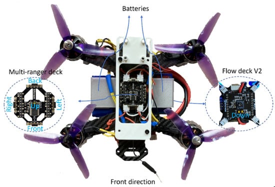
Figure 1.
The quadcopter platform with attached sensors.

Table 1.
The key components of our quadcopter platform.
The multiranger deck is composed of five VL53L1x time-of-flight (TOF) range finders (1D scanners) to measure the distance in five different directions: front, back, left, right, and up (Figure 1). The Flow deck consists of the VL53L1x range finder, which measures the distance to the ground, and the PMW3901 (https://docs.px4.io/v1.11/en/sensor/pmw3901.html, accessed on 22 August 2022) tracking sensor, which measures movements in relation to the ground (Figure 1). The VL53L1x can measure ranges up to 4 m. The PMW3901 is adapted to work from approximately 80 mm to infinity, according to its specification.
The platform is equipped with four plastic propellers, electronic speed controllers (ESCs) and four SkyRC X2208 motors with a diameter of 28 mm, a length of 35 mm, and a weight of 37.5 g. The drone is supplied by two LiPo batteries with three cells, a nominal voltage of 11.1 V, a size of 57 × 30 × 23 mm, a weight of 70 g, and a minimum capacity of 800 mAh. The batteries provide energy for up to 12 minutes of continuous flight. The total weight of the key components, including the structure of the drone (52 g), is 401.5 g.
This nanoflying drone depends on two microcontrollers. The first is NRF51, which handles radio communication and power management. The second is the STM32F405, which handles the sensor reading, motor, and flight control. The microdrone communicates with a PC computer (ground station) over the Crazyradio PA USB radio dongle within a range line-of-sight of up to 1 km. The drone streams data to the ground station using the onboard nRF radio module. We used the ground station keyboard for manual control. The proposed microdrone uses the Flow deck and multiranger deck to measure the distance in all directions and avoid obstacles, as explained in our previous work [8]. The cost of the whole drone, including a flight controller (Crazyflie Bolt 1.0), is approximately 550 USD, and it can take a week to build it.
3.2. Sensor Data Fusion
Multisensor mobile mapping devices often employ three different coordinate systems: the sensor system, the body frame system, and the world system (local or global). In our drone, each range finder records data with its own sensor system. To integrate the data of the six rangers, their sensor systems had to be transformed into a unified frame system. We adopted the Flow deck system as the body frame system of the presented UAV. The positive x-axis runs along the front direction of the frame object, the positive y-axis runs along the left direction of the frame object, and the positive z-axis points upward and perpendicular to the xy-plane.
The multiranger deck is positioned horizontally above the Flow deck and in such a way that the front, back, left, and right laser rangers face in the positive and negative direction of the x- and y-axis of the frame system, respectively (Figure 1). Assuming that all the sensors are rigidly mounted on the platform, the six laser points that are captured by the six laser rangers (= up, down, left, right, front or back) at each timestamp are defined in the body frame system () as follows:
where and are translation parameters from the laser rangers to the frame system () and index points.
Note that, in the rest of the paper and for simplification purposes, we omitted the laser ranger index from the laser point name . The following equations are applied to all laser points regardless of the measurement ranger.
Since the body frame system moves constantly with the drone, we defined a fixed local world system in which the final point cloud and trajectory are registered. This world system is assumed to be the body frame system at the starting pose. Accordingly, the laser points can be transformed to the world system () by:
where and are the time-dependent rotation matrix and translation from the body frame system () to the world system (), respectively.
3.3. Planar Segment Extraction
As our drone is equipped with 1D scanners, the recorded laser data per timestamp are not sufficient to extract planar segments. Therefore, we utilized the EKF-predicted point cloud to extract planar segments (Figure 2).
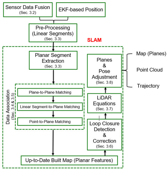
Figure 2.
The overall concept of the proposed methodology.
Due to the architecture of the side range finders (Figure 1), the recorded points while flying the drone are distributed almost linearly on the surrounding walls. Therefore, we detected the linear segments in the predicted point cloud independently for each side ranger by using a line segmentation algorithm [48], and then extracted the planar segments based on the linear segments, assuming the walls to be vertical (Figure 3). For the vertical rangers, the planar segments were extracted using a surface-growing segmentation [49].
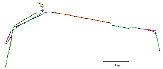
Figure 3.
Top view of the laser points captured by the left ranger on the left walls of a corridor. The colors show the plane association, and the black lines refer to the extracted planes (2D bounding boxes).
To increase the robustness of the planar segment extraction, we filtered out the linear segments and planar segments based on several thresholds: the length threshold , point threshold and standard deviation threshold. We extracted a plane from a linear segment whose length was greater than , had a number of points higher than and had a relatively low standard deviation of line-fitting residuals (lower than 5 cm). Moreover, a plane was filtered out if the standard deviation of the plane fitting residuals was higher than .
We ensured that the normal vector of each extracted plane pointed towards the drone’s location while scanning the corresponding planar structure. This was beneficial for plane-to-plane matching, as described in the next section. Moreover, from the points of each segment, we extracted a 2D bounding box, as shown in Figure 3. It is an oriented box based on the plane fitted to the corresponding points. It is worth mentioning that the bounding boxes of the planar features in the generated maps were extended to the nearest corner for visualization purposes.
3.4. Plane-to-Plane Matching
Since the employed SLAM is based on planar features, we used plane-to-plane matching as an essential technique for data association (Figure 2) and loop closure (Section 3.4). Two or more planar segments may represent the same planar structure in an interior space. To detect such planes, we looped over all the extracted planes, and for each plane, we searched for matching candidates. The selection of these candidates was based on a set of criteria. First, the distance between the tested plane and its candidates should not exceed a certain threshold (see Table 2). Second, the normal vectors of the tested plane and its candidates should point in the same direction. Third, there should be an overlapping area between the corresponding bounding boxes.
Table 2.
Thresholds and their value for the proposed methodology.
The planes that met these criteria were matched on one plane, which contained the points of both planes. A new bounding box was derived based on the extent of the new plane. Since the map was updated and the bounding boxes of some planes were extended, nearby planes may have started to overlap. Therefore, we iterated the plane-to-plane matching over the planes until no further candidates for matching were nominated. The proposed matching technique decreased the number of planes in the built map, thereby reducing the complexity of the map and speeding up the optimization process.
3.5. Linear Segment-to-Plane and Point-to-Plane Matching
We checked the association between the leftover linear segments that did not satisfy the requirements to instantiate a plane (Section 3.3) and the planes on the map (Figure 2). Similar to the previous association check, if the distance and angle between the segment and a plane were within a given limit and their 2D bounding boxes overlapped, the segment’s points were associated with this plane and the plane’s bounding box was updated based on the added points. The laser points that were not assigned to a linear segment or a planar segment were associated with their closest planes on the map (Figure 2). A point was added to a plane if it was located within its bounding box and within a certain distance (see Table 2).
It is worth mentioning that the bounding boxes of the planar features in the generated maps were extended to the nearest corner for visualization purposes. Using the vertical ranger-based planes (Section 3.3), we determined the heights of the ceiling and floor surfaces and extended the wall planes (i.e., 2D bounding boxes) to the corresponding floor and ceiling levels.
3.6. Loop Closure
The loop-closure detection and correction technique applied in this study is similar to the ones presented in our previous work [29] for a wearable mapping system, except for differences in the detection process. In contrast to wearable systems, which observe surrounding spaces from fixed operator-based altitudes, drones observe spaces from different altitudes. Since our UAV records the linear points on the surrounding walls, a pair of planes may represent the same planar structure, but their bounding boxes do not spatially overlap in 3D space. Therefore, we applied score-based loop-closure detection, which considers the overlap between two bounding boxes as an indicator worthy of giving a score, although it is not a decisive criterion that requires plane-to-plane matching.
Specifically, the detection approach is used to search for planes that meet a set of criteria. Although the first three criteria are identical to the ones in plane-to-plane matching, addressed above (Section 3.4), we relaxed the distance and angle thresholds to compensate for the larger expected accumulation of drift in the loop-closure area. The fourth criterion is the overlap between the bounding boxes not only in 3D space, but also in 2D planes, namely the YZ and XZ planes. For the fifth criterion, the tested planes were observed at separate time intervals, as the drone was expected to fly around in the target space before returning to the loop-closure area. For the sixth criterion, the bounding boxes were in proximity.
We assigned a score of one to a pair of planes for each criterion they met. A higher score was assigned to the pair of planes that met a combined criterion, e.g., the distance and angle criteria together. At the end, the pairs of planes with the highest scores were selected as the most probable locations for the loop closure. Next, the loop-closure correction merged these planes and modified the graph.
3.7. LiDAR Observation Equation
Each point assigned to a plane has two attributes: plane number and residual. The term residual refers to the distance between the point and the plane to which the point belongs. The LiDAR observation equation is formulated for each assigned point based on the expectation that the point’s residual equals zero (Figure 2).
where is the plane’s normal vector and is the signed distance to the plane , . is the azimuth angle and is the angular parametrization of plane ; it is used in the final formulation of the observation equation, Equation (10).
However, the residual is not necessarily zero because of the sensor noise and the accumulated drift over time.
Since LiDAR points are recorded in the body frame system, Equation (4) can be rewritten based on Equation (2), as follows:
The drone pose parameters () are modeled as functions of time using splines. For instance, is formulated as follows:
where is the spline coefficient for to be estimated on interval and is the B-spline value at time on interval .
Consequently, the rotation and translation can be written as follows:
The employed SLAM is a graph optimization problem that utilizes the LiDAR observations to estimate the map of the scanned space and the poses of the drone simultaneously. The state vector to be estimated can be formulated as follows:
where spline coefficients on interval .
We linearized the splines of the pose parameters. For instance, the linearized spline:
where the upper index denotes the approximate value.
After linearizing Equation (5) with respect to the unknown pose spline coefficients and unknown plane parameters using Taylor-series expansion, the LiDAR observation equation can be formulated as follows:
where , , , , are the unknown increments of the pose splines coefficients on interval and are the unknown increments of the plane parameters.
3.8. SLAM
The equation system in the adjustment (SLAM) consists of Equation (11) for all the points assigned to the planes and is solved by a least-squares solution to estimate the unknown increments containing the increments of all the plane parameters and spline coefficients. The SLAM solution seeks to minimize the sum of squared residuals :
where . refers to the number of points involved in the SLAM.
The plane and pose parameters in the state vector are updated using the increments , Equation (13). The SLAM iterates and all the planes and splines (and, thus, the points’ locations) are updated until convergence (Figure 2).
where is the number of iterations.
However, the geometry of the LiDAR observations captured by the proposed flying drone is sometimes not enough to reliably estimate the 3D pose of the drone. The problem itself is generic, but its impact on the ability to estimate our drone’s pose is significant due to the limited features of our sensor configuration. To overcome this problem, we added stabilization equations that maintained the approximate values of the spline coefficients and prevented the drone from sliding in any direction.
4. Experiments
Below, we briefly describe the test sites (Section 4.1) and present the experimental results (Section 4.2). The point clouds included some outlying points, which were captured through glass. Since these points were often not present in both clouds, we excluded them from the comparison.
To evaluate the quality of the resulting maps, we compared the generated point clouds to those obtained by the MAX drone [22], IPS [33] and the RIEGL VZ-400 TLS as the ground truth (Section 4.4). Next, we compared the computed distances in the resulting map with the floor plan (Section 4.5).
MAX is a research quadcopter macrodrone developed by the Swedish Defense Research Agency (FOI). Its platform is equipped with an Ouster LiDAR with a 100-meter range, and a stereo camera with a 10-m range. The MAX drone employs two independent positioning systems: a camera-based system and a LiDAR-based system [8,22]. The MAX point clouds used in this work were obtained from the latter system. Karam et al. [8] compared the LiDAR-based system against the TLS, and the results showed that MAX experienced a deviation of 50 cm along the x and y axes for a traveled distance of approximately 65 m in an indoor office environment.
IPS is a vision-aided navigation system developed by the German Aerospace Center (DLR). It is a wearable platform in the shape of a helmet that features a mounted IMU and stereo camera. The IPS can be fused with global navigation satellite systems (GNSSs), which makes it applicable to indoor–outdoor scenarios [33]. The measurements presented by Börner et al. [33] demonstrated that the IPS led to a 3D error of 40 cm over a 400-m long acquisition trajectory in a typical indoor environment.
4.1. Test Sites
We collected the data from three different test sites. At each site, we selected the mapping scenario in such a way that the operator could not see the observed space from the take-off location.
The first, second and third datasets, named ITC1, ITC2 and ITC3, were collected at the University of Twente, Faculty of Geo-Information Science and Earth Observation (ITC) building in Enschede, the Netherlands. ITC1 is a corridor in the form of an L-shaped hexagon (Figure 4 and Figure 5), while ITC3 is a loop around an irregularly shaped room (Figure 6. The ITC1 and ITC2 (Figure 7) datasets were used to evaluate the performance of the proposed methodology in indoor mapping, against the ground truth obtained by the RIEGL TLS (Figure 5) and floor plan, respectively.
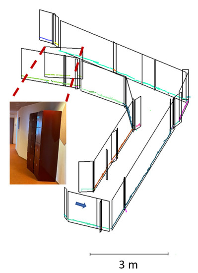
Figure 4.
Slanted view of our point cloud (colors show plane association) with wall planes (black lines) for the ITC1 dataset. The blue arrow refers to the starting position and the dashed red lines refers to a cupboard located in the corridor. The ceiling and floor points are not shown for visualization purposes.
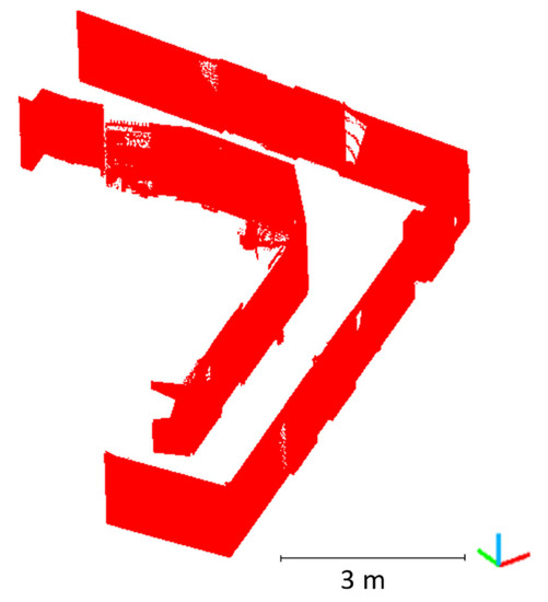
Figure 5.
Slanted view of the TLS 3D point cloud for the ITC1 dataset. The ceiling and floor points are not shown for visualization purposes.
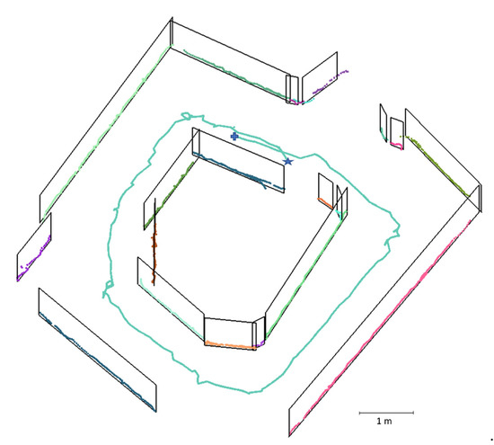
Figure 6.
Slanted view of our point cloud (colors show plane association) with wall planes (black lines) for the ITC3 dataset. The blue star and plus signs refer to the start and end of the trajectory (turquoise), respectively. The ceiling and floor points are not shown for visualization purposes.
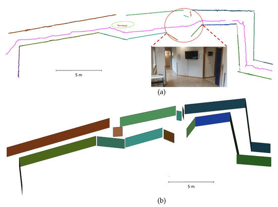
Figure 7.
Our map for the ITC2 dataset. (a) Top view of our point cloud (colors show plane association) with wall planes (black lines). The floor’s points are not shown for visualization purposes. The green oval surround a pillar in the corridor. The dashed red lines refers to the corresponding space in the corridor. (b) Slanted view of our map (colored bounding boxes refer to the 3D planar features).
The fourth dataset, named Apartment, was collected in a corridor in a typical student apartment in Münster, Germany. Similar to the ITC datasets, we utilized this dataset to evaluate the performance of our drone in mapping indoor spaces, and to compare some distances in our map with the corresponding distances in the floor plan (Figure 8).
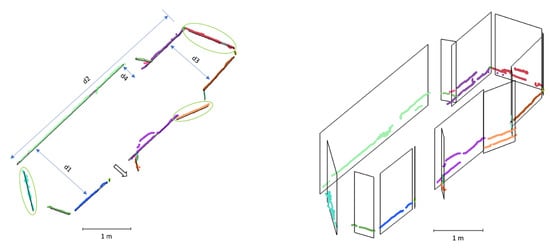
Figure 8.
Top view (left) and slanted view (right) of our point cloud for the Apartment dataset. Colors show plane association. The ceiling’s and floor’s points are not shown for visualization purposes. The black 2D bounding boxes represent the reconstructed planes. The green ovals surround the opening doors, the blue arrows refer to distance measurements, and the black arrow points to an opening into another space.
The fifth and sixth datasets, named DLR1 and DLR2, respectively, were captured indoors at the German Aerospace Center (DLR) premises in Berlin, Germany. The DLR1 dataset was obtained from a corridor and a printer room that were connected through a wide-open door (Figure 9). The DLR2 dataset was captured in an almost U-shaped space (Figure 10). These datasets were used to contrast the performance of the proposed methodology in indoor mapping against those of the IPS helmet and MAX drone. Similar to the Apartment dataset, we compared some distances on our map with the corresponding distances in the floor plan (Table 3).
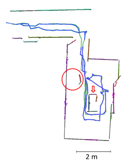
Figure 9.
Top view of our point cloud (colors show plane association) with wall planes (black lines) for the DLR1 dataset. The ceiling points (blue) and floor points (green) overlap in the middle of the scanned space. The red circle refers to an object (printer), and the red arrow points to a cupboard; see Figure 11.
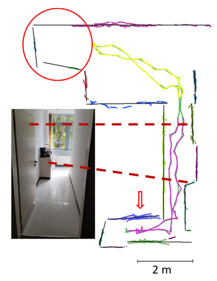
Figure 10.
Top view of our point cloud (colors show plane association) with wall planes (black lines) for the DLR2 dataset. The points at two different heights of the ceiling (yellow and pink) and floor points (green) overlap in the middle of the scanned space. The red circle refers to an area not visited by our drone, and the red arrow points to the kitchen space. The dashed red lines refer to the corresponding objects in the kitchen.
Table 3.
Distances from our point cloud against a reference floor plan.
Furthermore, the DLR1, DLR2 and ITC3 experiments aimed at demonstrating the ability of our SLAM to detect and correct loop closure. Therefore, in these experiments, the drone returned to the take-off location.
For comparison purposes, our drone and the MAX had the same initial location and orientation and operated at almost the same flight height during mapping. Moreover, the point clouds of all the systems—our drone, the IPS, the MAX and the TLS—were registered in the same coordinate system, using rigid transformation. The registration process was performed by means of course registration and the iterative closest points (ICP) algorithm included in the open-source, free software CloudCompare (http://www.cloudcompare.org/).
For the experiments, the thresholds used are listed in Table 2. We set to 10 for the minimum number of points in a linear segment. The length threshold was set to 15 cm, and the angle and distance thresholds for the data association in the proposed SLAM were 10° and 20 cm, respectively. For the loop closure, these thresholds were relaxed to 22° and 1 m, respectively. The maximum standard deviation of line and plane fitting residuals of points were set to 5 cm and 30 cm, respectively. These thresholds were experimentally determined.
4.2. Appearance–Reality Distinction
Figure 4, Figure 6, Figure 7, Figure 8, Figure 9 and Figure 10 show the point clouds generated with the proposed SLAM for the ITC1, ITC3, ITC2, Apartment, DLR1, and DLR2 datasets, respectively. As the proposed microdrone was built out of 1D scanners with a limited field of view and range (<4 m), it was worth investigating the ability of the employed SLAM to provide an exploration map through which to quickly obtain the indoor space shapes. Indeed, the ability of our method to provide a recognizable shape of the scanned space is evident in Figure 4, Figure 6, Figure 7, Figure 8, Figure 9 and Figure 10. The L-shape of the ITC1 dataset and the almost-U-shape of DLR2 can easily be recognized in Figure 4 and Figure 10. The corridor in the Apartment dataset has four openings; one has no door (indicated by the black arrow in Figure 8) and the other three have half-open doors (indicated by the green ovals in Figure 8).
In Figure 5, the shape of the mapped space is clear in the TLS point clouds, and the details are accurate and sharp. However, the planar features in Figure 4 also make the shape of the space clear on our map. A visual inspection of the generated map showed that our feature-SLAM-based microdrone provided a comparable map to that of the TLS, because the microdrone-derived point cloud with planar features (Figure 4) was geometrically similar to the TLS point cloud (Figure 5).
Similarly, our point clouds for the DLR datasets (Figure 9 and Figure 10) were geometrically similar to the corresponding point clouds derived by the MAX drone (Figure 11) and the IPS helmet (Figure 12). Moreover, Figure 12 demonstrates that our point clouds depicted the geometry of the DLR sites more precisely than the IPS point clouds.
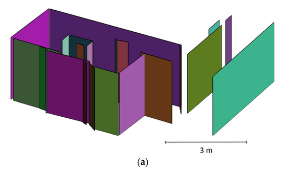
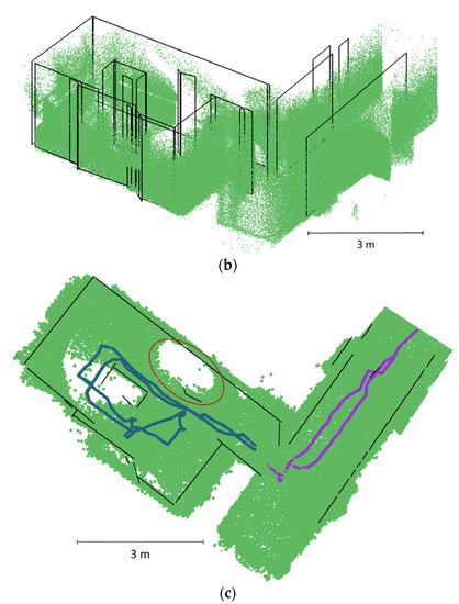
Figure 11.
The MAX and our map for the DLR1 dataset. (a) Slanted view of our map (the colored bounding boxes refer to the 3D planar features). (b) Slanted view of the MAX 3D point cloud (green) and our map (the black bounding boxes refer to the 3D planar features). (c) Top view of the MAX 3D point cloud (green) and our map (the black bounding boxes refer to the 3D planar features) with points at two different heights of the ceiling (blue and purple). The red circle refers to an object (printer).
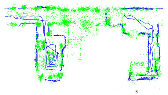
Figure 12.
Top view of the IPS 3D point cloud (green) and our point clouds (blue) for the DLR datasets.
Figure 9, Figure 10 and Figure 11 show that some details are more recognizable on our map than on that of the MAX, and vice versa. For instance, the cupboard in the middle of the room in Figure 11 was reconstructed with a clearer layout on our map compared to that of MAX, while the layout of the printer is clearer on the MAX map compared to ours (as indicated by the red circle in Figure 11c). Similarly, the layout of the kitchen is clearer on our map (Figure 10). However, during the data collection, our drone became less stable and began to wobble in the kitchen area. This is reflected by the sparser points on our map of the kitchen compared to other areas (the red arrow in Figure 10). The main reason for this discrepancy is related to the fact that the floor of the kitchen was highly reflective, and the Flow deck performs relatively poorly over such surfaces. This is because optical-flow sensor-based 2D positioning is highly affected by the number of visual features and the light conditions in the flight area.
The red circle in Figure 10 refers to a spot in the corridor that was unvisited by our drone. Therefore, there was a lack of LiDAR observations, which in turn led to an incomplete and inaccurate reconstruction compared to the corresponding part in the MAX map.
The same applies to the end of the corridor in the DLR1 dataset, which was not visited by our drone (Figure 9); by contrast, this area was reconstructed properly by the MAX due to its longer-range sensors. The second reason for this discrepancy was that our forward ranger observed the glass part of the door. This problem could have been overcome by rotating the drone around the z-axis to capture as many points as possible on the surfaces at the end of that corridor.
One of the key advantages of our drone is its capability to capture the ceiling and floor independently from the operating height. This was evident through the ability of our UAV to capture the ceiling in all the experiments. Moreover, our SLAM showed the ability to detect the change in the ceiling height in the DLR datasets and segment the ceiling points into different planar features (Figure 9, Figure 10 and Figure 11), although the variance in the height of the ceiling was less than 20 cm.
4.3. Cloud-to-Cloud Comparison
To quantify the deviation of our point clouds from the compared clouds, we computed the cloud-to-cloud absolute distances (C2C), as shown in Table 4 and Figure 13. The C2C distances were computed in two cases: with and without the SLAM (i.e., predicted point clouds) in order to evaluate the benefits of the SLAM for map generation.
Table 4.
C2C distances between our drone and the compared systems (TLS and MAX).
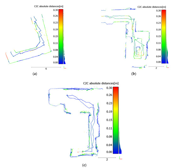
Figure 13.
Our point clouds are colored based on C2C distances from the TLS map for the ITC dataset (a), and from the MAX map for the DLR1 (b) and DLR2 (c) datasets.
The microdrone-TLS comparison results showed that, on average, approximately of the C2C distances were less than 10, and that approximately of the distances were less than 20 cm. The percentage of the C2C distances that were less than 20 cm differed slightly when the SLAM was executed, while the SLAM significantly increased the percentage of the distances that were less than 10 cm (from 48% to 75%). Thus, the SLAM improved the accuracy of the generated point cloud, while the deviation of the point cloud from the ground truth was significantly lower than that obtained without the SLAM.
Compared to the MAX, our drone showed comparable performance due to the low deviation of our point cloud from the one obtained by the MAX. The majority of the cloud-to-cloud distances were less than 10 cm. It is worth mentioning that the ceiling points were excluded from the C2C computation because the MAX point cloud had no points on the ceiling.
Similar to the MAX, the IPS point cloud had no points on the ceiling. Moreover, the IPS cloud had a lower density on the walls than our point cloud (Figure 12). Since the reference point cloud in the C2C calculation should have a higher density than the point cloud with which it is compared, we did not compute the C2C distances between our cloud and the IPS cloud, as it would have yielded a biased estimation of the real deviation between the two clouds.
4.4. Floor Plan Comparison
To further evaluate the performance of the proposed methodology, we computed some of the distances between the planar features in the resulting map for the Apartment dataset and compared them against the corresponding measurements in the floor plan, as illustrated in Figure 8 and Table 3. Similarly, we compared the distances , and in the DLR1, DLR2 and ITC2 datasets, respectively (Table 3).
Table 3 shows that the distance differences were less than 20 cm in the DLR1 and DLR2 datasets and up to approximately 30 cm in the ITC2 dataset. The reduced accuracy in the ITC2 dataset can be explained as a distribution of larger accumulated drift over a longer trajectory. Additionally, the floor of the corridor was highly reflective, similar to the kitchen in DLR2.
We did not consider the errors in the floor plan. Assuming the floor plan as reference data, the comparison showed that the distance accuracy at the take-off location was stronger than at the landing location. This was consistent with the expected performance of the SLAM algorithms. In other words, in contrast to which differed from the floor plan by 8 cm, the difference in was less than 3 cm because it was measured in the starting location of the drone and was, thus, affected only minimally by the cumulative drift from which SLAM-based point clouds usually suffer over time.
4.5. Analysis of Loop-Closure Technique’s Performance
Figure 6 shows the generated map for the ITC3 dataset. The drone took off from the location marked by the blue star sign, hovered around a room that has an irregular layout, and landed at the marked location by the blue plus sign. The accumulated drift at the end of the loop without any loop closure correction (Figure 14a) was on average 2.7% (0.65 m) and 0.1 °/m over a 23.8-m long acquisition trajectory. Figure 14a shows that, without a loop closure, reobserving places introduces duplicate walls into the map. The corresponding planes were merged, and the loop closure was corrected within our SLAM, as shown in Figure 14b.
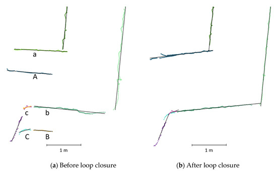
Figure 14.
The loop in the ITC building (ITC3 dataset). (a) Top view of the wall points with planes (black lines) at the start (a–c) and end (A–C) of the loop without loop closure. (b) The wall points and the planes after loop closure correction. Point colors show plane association.
In the DLR datasets, the drone hovered at two different heights and returned to the take-off location. On the one hand, this led to more laser points on the surrounding planar structures and, therefore, provided a more reliable estimation of the planar features. On the other hand, the laser data on the same planar structure were not aligned due to the cumulative drift over time. The largest drift was observed in the loop-closure area. The results showed a drift of an average of 1.1% (0.35 m) and 0.41°/m over a 31-m-long acquisition trajectory.
The drift was mainly in the moving direction, i.e., the direction of the x- and y-axis. Although the drone moved up and down in the z-axis direction during the data collection, the resulting drift in the z-axis direction was minor and smaller than the data association threshold. Therefore, the drone still observed the previously estimated planes for the ceiling and floor while returning to the take-off location.
The resulting drift in orientation was mainly around the z-axis, which represented the rotation direction while scanning. Due to the limited range and field of view, we need to rotate the drone around the z-axis while moving to cover as much as possible of the surrounding space. This rotation led to a larger drift in orientation. A small error in the orientation can have serious effects on the quality of the data association. As a simple example, if there was a LiDAR point at a distance of from the drone, a drift in the orientation of the kappa angle () of one sigma 1° would result in a 7-cm lateral displacement of this point. However, our scoring-based loop-closure technique managed to detect the loop closure and correct the drift over the entire map, as shown in Figure 6, Figure 9 and Figure 10.
4.6. Discussion
The results demonstrated that the proposed SLAM could handle the test sites and generate point clouds successfully for all the datasets in this study. The proposed SLAM is relatively hardware-independent and not limited to the customized microdrone used in this work. The main change required for a different LiDAR sensor configuration is in the planar segment extraction (Section 3.3). For instance, a multilayer LiDAR (such as Velodyne)-based drone can extract the planar segments (if present) from a single scan without the need to collect successive scans.
However, our drone is significantly smaller than the common multilayer LiDAR-based drones and, thus, can access indoor spaces that are inaccessible to those drones. Nevertheless, this comes at the expense of a less flexible hardware and less coverage of the surrounding space.
Flying a 1D scanner-based drone, such as the one used in this study, at different heights, can help to cover a wider area of the planar structure. This, then, may allow for a more accurate hypothesis of the planar structures, free of assumptions about the horizontal and vertical planes. However, in our experiment, our drone’s drift was significant and larger than the data association threshold, which made it difficult to distinguish whether the misalignment between the laser data at two different levels resulted from the drift over time or from the location of the data along a slanted surface. Therefore, we assumed that the walls were vertical, which is common in man-made indoor environments, and overly relaxed the data association thresholds to correct the accumulated drift. The main source of the drift could have been the flow-deck-based positioning system, which experienced difficulties tracking sufficient visual features on the ground surface of the scanned spaces.
Moreover, we experimentally found that there is a limitation in the operational range of the optical flow sensor. Therefore, we recommend flying the drone at a relatively low height above the floor (0.30–2.00 m) for stable hovering.
Our loop-closure technique modifies the graph to correct the cumulative drift by using plane-to-plane matching. Since the planar features are large (see Section 3.3) and spatially distinct, and the scoring-based method involves extensive checks to determine the pair of planes to be matched, the risk of merging the incorrect planes is almost negligible.
5. Conclusions
In this paper, we presented and experimentally validated a planar-feature-based SLAM algorithm on a customized microdrone for indoor mapping. Our SLAM algorithm combined plane-to-plane matching for data association with graph optimization to estimate the state of the drone and the SLAM map, and performed loop-closure detection and correction. The proposed mapping system is based on a simple combination of 1D scanners and, thus, our sensor package is simpler than those used in comparable systems.
Our drone was able to map all test sites used in this study, and provide maps in the shape of point clouds, which provided sufficient information for exploration purposes. The experimental results showed the promising performance of our drone in mapping small indoor spaces. This was evident from the relatively low deviation between our point cloud and those derived from the systems to which it was compared: the MAX drone, the IPS helmet, and the TLS. Moreover, the comparison with the floor plan showed that the distance differences did not exceed 15 cm.
The presented platform is customizable in terms of sensor arrangement, meaning that additional complementary sensors can be added. In future work, we intend to integrate complementary sensors, such as a thermal camera, to expand the scope of application of our drone to include, for example, victim detection applications. Moreover, propeller guards could be added to our platform to reduce the chance of the drone crashing in case of contact with surrounding objects.
Moreover, adding another source of navigational information to the onboard positioning system can support the drone in overcoming textureless spots, which in turn improves the localization and orientation accuracy, specifically the orientation around the z-axis. For example, the capacity of our drone allows for adding a small IMU and more laser rangefinders. The additional laser rangers can be tilted (i.e., at slanted angles) and mounted in the existing gaps to the left and right of the side laser rangers in the presented design. Using slanted angles appears as a minor detail, but it can lead to better coverage of the walls around the drone, which in turn makes the estimation of planar features more robust. This improvement could enable the drone to handle indoor spaces with arbitrarily oriented planes, such as staircases.
Additionally, the proposed methodology was applied offline, and we intend to run it online to make the correction of accumulated drift more efficient over time. This could enable our SLAM algorithm to handle a multiple-loop scenario.
In addition, there is a trend towards the development of a new multiranger deck that uses the new multizone-ranging TOF scanner VL53L5CX (https://www.st.com/en/imaging-and-photonics-solutions/vl53l5cx.html, accessed on 15 September 2022). The new scanner has a wide diagonal field of view of 63°. These changes may provide wide LiDAR scans similar to those produced by scanners with higher dimensions. These changes would benefit our SLAM algorithm by increasing its robustness and ability to handle more complex indoor environments.
Author Contributions
Conceptualization, S.K., F.N. and N.K.; methodology, S.K.; software, S.K.; hardware, S.K. and B.T.C.; validation, S.K.; formal analysis, S.K.; investigation, S.K.; resources, S.K. and B.T.C.; data curation, S.K.; writing—original draft preparation, S.K.; writing—review and editing, S.K., F.N., B.T.C. and N.K.; visualization, S.K.; supervision, F.N. and N.K.; project administration, F.N. and N.K.; funding acquisition, F.N. and N.K. All authors have read and agreed to the published version of the manuscript.
Funding
The INGENIOUS project has received funding from the European Union’s Horizon 2020 Research and Innovation Programme and the Korean Government under grant agreement No. 833435. The content reflects only the authors’ views. The Research Executive Agency (REA) and the European Commission are not responsible for any use that may be made of the information this manuscript contains.
Data Availability Statement
The data supporting the reported results were uploaded to Data Archiving and Networked Services (DANS), which promotes sustained access to digital research data (www.dans.knaw.nl), and they will be published soon.
Acknowledgments
We acknowledge Gustav Tolt, Oskar Karlsson and Joakim Rydell from the Swedish Defense Research Agency (FOI) for kindly providing the MAX point cloud. The authors would also like to thank Jürgen Wohlfeil and Adrian Schischmanow from the German Aerospace Center (DLR) for kindly providing the IPS point cloud.
Conflicts of Interest
The authors declare no conflict of interest.
References
- Kerle, N.; Nex, F.; Gerke, M.; Duarte, D.; Vetrivel, A. UAV-based Structural Damage Mapping: A review. ISPRS Int. J. Geo-Inf. 2019, 9, 14. [Google Scholar] [CrossRef]
- Alamouri, A.; Hassan, M.; Gerke, M. Development of a methodology for real-time retrieving and viewing of spatial data in emergency scenarios. Appl. Geomat. 2021, 13, 747–761. [Google Scholar] [CrossRef]
- INGENIOUS Project. Available online: https://ingenious-first-responders.eu/ingenious-project/ (accessed on 26 September 2022).
- Lin, Y.C.; Zhou, T.; Wang, T.; Crawford, M.; Habib, A. New Orthophoto Generation Strategies from UAV and Ground Remote Sensing Platforms for High-Throughput Phenotyping. Remote Sens. 2021, 13, 860. [Google Scholar] [CrossRef]
- Karam, S.; Vosselman, G.; Peter, M.; Hosseinyalamdary, S.; Lehtola, V. Design, Calibration, and Evaluation of a Backpack Indoor Mobile Mapping System. Remote Sens. 2019, 11, 978. [Google Scholar] [CrossRef]
- Pintore, G.; Pintus, R.; Ganovelli, F.; Scopigno, R.; Gobbetti, E. Recovering 3D Existing-Conditions of Indoor Structures from Spherical Images. Comput. Graph. 2018, 77, 16–29. [Google Scholar] [CrossRef]
- Dowling, L.; Poblete, T.; Hook, I.; Tang, H.; Tan, Y.; Glenn, W.; Unnithan, R.R. Accurate Indoor Mapping Using an Autonomous Unmanned Aerial Vehicle (UAV). arXiv 2018. [Google Scholar] [CrossRef]
- Karam, S.; Nex, F.; Karlsson, O.; Rydell, J.; Bilock, E.; Tulldahl, M.; Holmberg, M.; Kerle, N. Micro and Macro Quadcopter Drones for Indoor Mapping to Support Disaster Management. ISPRS Ann. Photogramm. Remote Sens. Spat. Inf. Sci. 2021, V-1-2022, 203–210. [Google Scholar] [CrossRef]
- Wang, F.; Cui, J.-Q.; Chen, B.-M.; Lee, T.H. A Comprehensive UAV Indoor Navigation System Based on Vision Optical Flow and Laser FastSLAM. Acta Autom. Sin. 2013, 39, 1889–1899. [Google Scholar] [CrossRef]
- Maboudi, M.; Homaei, M.; Song, S.; Malihi, S.; Saadatseresht, M. A Review on Viewpoints and Path-planning for UAV-based 3D Reconstruction. arXiv 2022. [Google Scholar] [CrossRef]
- Nex, F.; Armenakis, C.; Cramer, M.; Cucci, D.A.; Gerke, M.; Honkavaara, E.; Kukko, A.; Persello, C.; Skaloud, J. UAV in the advent of the twenties: Where we stand and what is next. ISPRS J. Photogramm. Remote Sens. 2022, 184, 215–242. [Google Scholar] [CrossRef]
- Zingg, S.; Scaramuzza, D.; Weiss, S.; Siegwart, R. MAV navigation through indoor corridors using optical flow. In Proceedings of the IEEE International Conference on Robotics and Automation 2010, Anchorage, AK, USA, 3–7 May 2010; pp. 3361–3368. [Google Scholar] [CrossRef]
- Yang, Y.; Geneva, P.; Eckenhoff, K.; Huang, G. Degenerate Motion Analysis for Aided INS with Online Spatial and Temporal Sensor Calibration. IEEE Robot. Autom. Lett. 2019, 4, 2070–2077. [Google Scholar] [CrossRef]
- Karam, S.; Lehtola, V.; Vosselman, G. Integrating a Low-cost MEMS IMU into a Laser-based SLAM for Indoor Mobile Mapping. Int. Arch. Photogramm. Remote Sens. Spat. Inf. Sci.—ISPRS Arch. 2019, 42, 149–156. [Google Scholar] [CrossRef]
- Sarker, M.; Kumar Sharma, N. Classification of Drones. Am. J. Eng. Res. 2013, 2, 19–38. [Google Scholar]
- Bailey, T.; Durrant-Whyte, H. Simultaneous Localization and Mapping (SLAM): Part II. IEEE Robot. Autom. Mag. 2006, 13, 108–117. [Google Scholar] [CrossRef]
- He, L.; Wang, X.; Zhang, H. M2dp: A Novel 3D Point Cloud Descriptor and its Application in Loop Closure Detection. In Proceedings of the IEEE International Conference on Intelligent Robots and Systems (IROS), Daejeon, Korea, 9–14 October 2016; pp. 231–237. [Google Scholar] [CrossRef]
- Ajay Kumar, G.; Patil, A.K.; Patil, R.; Park, S.S.; Chai, Y.H. A LiDAR and IMU Integrated Indoor Navigation System for UAVs and its Application in Real-Time Pipeline Classification. Sensors 2017, 17, 1268. [Google Scholar] [CrossRef]
- Le Gentil, C.; Vidal-Calleja, T.; Huang, S. IN2LAMA: Inertial Lidar Localisation and Mapping. In Proceedings of the IEEE International Conference on Robotics and Automation 2019, Montreal, QC, Canada, 20–24 May 2019; pp. 6388–6394. [Google Scholar] [CrossRef]
- Cui, J.Q.; Phang, S.K.; Ang, K.Z.Y.; Wang, F.; Dong, X.; Ke, Y.; Lai, S.; Li, K.; Li, X.; Lin, F.; et al. Drones for Cooperative Search and Rescue in Post-Disaster Situation. In Proceedings of the 2015 7th IEEE International Conference on Cybernetics and Intelligent Systems CIS and 2015 IEEE Conference on Robotics, Automation and Mechatronics, RAM 2015, Siem Reap, Cambodia, 15–17 July 2015; pp. 167–174. [Google Scholar] [CrossRef]
- Gao, F.; Wu, W.; Gao, W.; Shen, S. Flying on Point Clouds: Online Trajectory Generation and Autonomous Navigation for Quadrotors in Cluttered Environments. J. Field Robot. 2019, 36, 710–733. [Google Scholar] [CrossRef]
- Tulldahl, M.; Holmberg, M.; Karlsson, O.; Rydell, J.; Bilock, E.; Axelsson, L.; Tolt, G.; Svedin, J.A. Laser Sensing from Small UAVs. In Proceedings of the Electro-Optical Remote Sensing XIV, Virtual, 21–25 September 2020; SPIE, the International Society for Optics and Photonics: Bellingham, WA, USA, 2020; Volume 11538, p. 115380C. [Google Scholar] [CrossRef]
- Ji, S.; Qin, Z.; Shan, J.; Lu, M. Panoramic SLAM from a Multiple Fisheye Camera Rig. ISPRS J. Photogramm. Remote Sens. 2020, 159, 169–183. [Google Scholar] [CrossRef]
- Lin, J.; Zheng, C.; Xu, W.; Zhang, F. R2LIVE: A Robust, Real-time, LiDAR-Inertial-Visual Tightly-coupled State Estimator and Mapping. IEEE Robot. Autom. Lett. 2021, 6, 7469–7476. [Google Scholar] [CrossRef]
- Grisetti, G.; Kümmerle, R.; Stachniss, C.; Burgard, W. A Tutorial on Graph-Based SLAM. IEEE Intell. Transp. Syst. Mag. 2010, 2, 31–43. [Google Scholar] [CrossRef]
- Lagmay, J.M.S.; Jed Leyba, L.C.; Santiago, A.T.; Tumabotabo, L.B.; Limjoco, W.J.R.; Michael Tiglao, N.C. Automated Indoor Drone Flight with Collision Prevention. In Proceedings of the IEEE Region 10 Annual International Conference/TENCON 2018, 28-Jeju, Jeju, Korea, 31 October 2018; pp. 1762–1767. [Google Scholar] [CrossRef]
- Raja, G.; Suresh, S.; Anbalagan, S.; Ganapathisubramaniyan, A.; Kumar, N. PFIN: An Efficient Particle Filter-Based Indoor Navigation Framework for UAVs. IEEE Trans. Veh. Technol. 2021, 70, 4984–4992. [Google Scholar] [CrossRef]
- Greiff, M. Modelling and Control of the Crazyflie Quadrotor for Aggressive and Autonomous Flight by Optical Flow Driven State Estimation. Master’s Thesis, Department of Automatic Control, Lund University, Lund, Sweden, 2017; p. 153. [Google Scholar]
- Karam, S.; Lehtola, V.; Vosselman, G. Simple Loop Closing for Continuous 6DOF LIDAR&IMU Graph SLAM with Planar Features for Indoor Environments. ISPRS J. Photogramm. Remote Sens. 2021, 181, 413–426. [Google Scholar] [CrossRef]
- Karam, S.; Lehtola, V.; Vosselman, G. Strategies to Integrate IMU and LIDAR SLAM for Indoor Mapping. ISPRS Ann. Photogramm. Remote Sens. Spat. Inf. Sci. 2020, V-1–2020, 223–230. [Google Scholar] [CrossRef]
- Le Gentil, C.; Vidal-Calleja, T.; Huang, S. IN2LAAMA: Inertial Lidar Localization Autocalibration and Mapping. IEEE Trans. Robot. 2020, 37, 275–290. [Google Scholar] [CrossRef]
- Nikoohemat, S.; Diakité, A.A.; Zlatanova, S.; Vosselman, G. Indoor 3D reconstruction from Point Clouds for Optimal Routing in Complex Buildings to Support Disaster Management. Autom. Constr. 2020, 113, 103109. [Google Scholar] [CrossRef]
- Börner, A.; Baumbach, D.; Buder, M.; Choinowski, A.; Ernst, I.; Funk, E.; Grießbach, D.; Schischmanow, A.; Wohlfeil, J.; Zuev, S. IPS-a Vision Aided Navigation System. Adv. Opt. Technol. 2017, 6, 121–129. [Google Scholar] [CrossRef]
- Paliotta, C.; Ening, K.; Albrektsen, S.M. Micro Indoor-Drones (MINs ) for Localization of First Responders. In Proceedings of the 18th ISCRAM, Blacksburg, VA, USA, 20–23 May 2021; pp. 881–889. [Google Scholar]
- Duisterhof, B.P.; Krishnan, S.; Cruz, J.J.; Banbury, C.R.; Fu, W.; Faust, A.; de Croon, G.C.H.E.; Janapa Reddi, V. Tiny Robot Learning (tinyRL) for Source Seeking on a Nano Quadcopter. In Proceedings of the IEEE International Conference on Robotics and Automation, Xi’an, China, 30 May–5 June 2021; pp. 7242–7248. [Google Scholar] [CrossRef]
- Zhang, N.; Nex, F.; Vosselman, G.; Kerle, N. Training a Disaster Victim Detection Network for UAV Search and Rescue Using Harmonious Composite Images. Remote Sens. 2022, 14, 2977. [Google Scholar] [CrossRef]
- Nex, F.; Duarte, D.; Steenbeek, A.; Kerle, N. Towards Real-Time Building Damage Mapping with Low-Cost UAV Solutions. Remote Sens. 2019, 11, 287. [Google Scholar] [CrossRef]
- Diosi, A.; Kleeman, L. Laser Scan Matching in Polar Coordinates with Application to SLAM. In Proceedings of the 2005 IEEE/RSJ International Conference on Intelligent Robots and Systems. IROS 2005, Edmonton, AB, Canada, 2–6 August 2005; pp. 3317–3322. [Google Scholar] [CrossRef]
- Besl, P.; McKay, N. Method for registration of 3-D shapes; Robotics-DL Tentative, International Society for Optics and Photonics: Bellingham, WA, USA, 1992. [Google Scholar]
- Fang, Z.; Yang, S.; Jain, S.; Dubey, G.; Roth, S.; Maeta, S.; Nuske, S.; Zhang, Y.; Scherer, S. Robust Autonomous Flight in Constrained and Visually Degraded Shipboard Environments. J. Field Robot. 2017, 34, 25–52. [Google Scholar] [CrossRef]
- Giernacki, W.; Skwierczy, M.; Witwicki, W.; Kozierski, P. Crazyflie 2.0 quadrotor as a platform for research and education in robotics and control engineering. In Proceedings of the 22nd International Conference on Methods and Models in Automation and Robotics (MMAR), Miedzyzdroje, Poland, 28–31 August 2017; pp. 37–42. [Google Scholar] [CrossRef]
- Silano, G.; Iannelli, L. CrazyS: A Software-in-the-Loop Simulation Platform for the Crazyflie 2.0 Nano-Quadcopter. In Proceedings of the 26th Mediterranean Conference on Control and Automation (MED), Zadar, Croatia, 19–22 June 2018; pp. 1–6. [Google Scholar] [CrossRef]
- Bouabdallah, S.; Siegwart, R. Full Control of a Quadrotor. In Proceedings of the IEEE International Conference on Intelligent Robots and Systems 2007, San Diego, CA, USA, 29 October–2 November 2007; pp. 153–158. [Google Scholar] [CrossRef]
- Nithya, M.; Rashmi, M.R. Gazebo-ROS-Simulink Framework for Hover Control and Trajectory Tracking of Crazyflie 2.0. In Proceedings of the IEEE Region 10 Annual International Conference/TENCON 2019, Kochi, India, 17–20 October 2019; pp. 649–653. [Google Scholar] [CrossRef]
- Kang, K.; Belkhale, S.; Kahn, G.; Abbeel, P.; Levine, S. Generalization Through Simulation: Integrating Simulated and Real Data into Deep Reinforcement Learning for Vision-based Autonomous Flight. In Proceedings of the IEEE International Conference on Robotics and Automation 2019, Montreal, QC, Canada, 20–24 May 2019; pp. 6008–6014. [Google Scholar] [CrossRef]
- Krishnan, S.; Boroujerdian, B.; Fu, W.; Faust, A.; Reddi, V.J. Air Learning: An AI Research Platform for Algorithm-Hardware Benchmarking of Autonomous Aerial Robots. arXiv 2019, arXiv:1906.00421. [Google Scholar] [CrossRef]
- Polosky, N.; Gwin, T.; Furman, S.; Barhanpurkar, P.; Jagannath, J. Machine Learning Subsystem for Autonomous Collision Avoidance on a small UAS with Embedded GPU. In Proceedings of the IEEE 19th Annual Consumer Communications & Networking Conference (CCNC), Las Vegas, NV, USA, 8–11 January 2022; pp. 1–7. [Google Scholar] [CrossRef]
- Peter, M.; Jafri, S.R.U.N.; Vosselman, G. Line Segmentation of 2D Laser Scanner Point Clouds for Indoor SLAM based on a Range of Residuals. ISPRS Ann. Photogramm. Remote Sens. Spat. Inf. Sci. 2017, IV-2/W4, 363–369. [Google Scholar] [CrossRef]
- Vosselman, G.; Gorte, B.; Sithole, G.; Rabbani, T. Recognising Structure in Laser Scanner Point Clouds. Int. Arch. Photogramm. Remote Sens. Spat. Inf. Sci. 2004, 46, 33–38. [Google Scholar]


Publisher’s Note: MDPI stays neutral with regard to jurisdictional claims in published maps and institutional affiliations. |
© 2022 by the authors. Licensee MDPI, Basel, Switzerland. This article is an open access article distributed under the terms and conditions of the Creative Commons Attribution (CC BY) license (https://creativecommons.org/licenses/by/4.0/).