Synergistic Use of Sentinel-2 and UAV Multispectral Data to Improve and Optimize Viticulture Management

Abstract

The increasing use of geospatial information from satellites and unmanned aerial vehicles (UAVs) has been contributing to significant growth in the availability of instruments and methodologies for data acquisition and analysis. For better management of vineyards (and most crops), it is crucial to access the spatial-temporal variability. This knowledge throughout the vegetative cycle of any crop is crucial for more efficient management, but in the specific case of viticulture, this knowledge is even more relevant. Some research studies have been carried out in recent years, exploiting the advantage of satellite and UAV data, used individually or in combination, for crop management purposes. However, only a few studies explore the multi-temporal use of these two types of data, isolated or synergistically. This research aims to clearly identify the most suitable data and strategies to be adopted in specific stages of the vineyard phenological cycle. Sentinel-2 data from two vineyard plots, located in the Douro Demarcated Region (Portugal), are compared with UAV multispectral data under three distinct conditions: considering the whole vineyard plot; considering only the grapevine canopy; and considering inter-row areas (excluding all grapevine vegetation). The results show that data from both platforms are able to describe the vineyards’ variability throughout the vegetative growth but at different levels of detail. Sentinel-2 data can be used to map vineyard soil variability, whilst the higher spatial resolution of UAV-based data allows diverse types of applications. In conclusion, it should be noted that, depending on the intended use, each type of data, individually, is capable of providing important information for vineyard management.

1. Introduction

Precision Agriculture (PA) emerged as an approach to improve inputs and agronomic practices to reduce the heterogeneity that exists in agricultural fields [1]. Its definition is associated with the concept of the five “R”s, which consist of applying the right product, at the right time, in the right place, in the right way, and with the right amount [2]. The implementation of PA techniques in viticulture—commonly referred to as precision viticulture (PV)—is relatively recent [3]. The objectives of PV are to ensure sustainable production through the reduction and efficient use of energy, fertilizers, chemicals, and other inputs, to minimize production costs and to promote better quality and productivity management [4].

Resource optimization and the control of agricultural production processes can be achieved by monitoring the variability within an agricultural area, using remote [5] or proximal [6] sensing techniques that allow effective crop management [7]. Remote sensing has been widely applied in agriculture due to its versatility [5]. The imaging sensors carried on these platforms can obtain data from different parts of the electromagnetic spectrum, at different spatial and temporal resolutions [8]. For PV, remote sensing presents some peculiarities that emphasize the importance of spatial resolution, as it has a direct impact on distinguishing canopy geometry or vineyard variability [9]. Spaceborne platforms can be associated with some disadvantages (affected by clouds [10] and temporal flexibility [11]). Nevertheless, satellites have been gaining expressiveness in the agronomic field [12], due to spatial data resolution improvements and availability [13].

The technological improvements have provided notable advances in remote sensing, leading, among others, to the emergence of unmanned aerial vehicles (UAVs), offering the possibility of quickly acquiring field data at lower costs [14]. UAVs’ ability to acquire near-surface data allows for greater spatial resolution [13] and is less affected by clouds. Furthermore, its flexibility extends to the sensors used, view angles, spatial resolution, and acquisition frequency [11]. The main disadvantage of UAVs is their reduced ability to survey large areas [15]. For this reason, UAVs are generally suitable for small-to-medium-sized projects [4]. UAV flexibility enables to improve the temporal resolution, allowing to monitor variations on vegetation and soil characteristics over time [16]. In fact, most UAV-based methods used to monitor crops are based on vegetation indices (VIs), obtained from arithmetic combinations of two or more spectral bands [17], to monitor, analyze and spatially detect variations in plant structures [7], as well as biophysical parameters [18]. Regarding PV, more than 90 VIs have already been applied [19].

The Normalized Difference Vegetation Index (NDVI) [20] is one of the most effective VIs to remotely monitor vegetation growth and development [21]. A dense canopy with a healthy leaf surface will provide low reflectance values in the red region and high reflectance values in the near-infrared (NIR) region, resulting in positive NDVI values [22]. In PV, NDVI has proved to be a useful means to detect seasonal variability in the vigor and yield of grapevines [23,24], to identify grapevine damage [25], to assess heat stress [26], and promote variable rate fertilizer management [27,28]. These results can only be achieved if the data used are acquired at specific periods of the crop’s phenological cycle.

In order to determine the changes that occur during the phenological stages of grapevines, and to identify crop health status, NDVI must be calculated from spectral images with a certain temporal resolution. One option is the use of medium-resolution satellite data (such as the Copernicus Sentinel-2), which provide information on the general characteristics of the vegetation [29], allowing vigor characterization and the monitoring of large-scale interventions [30]. However, the use of Sentinel-2 multispectral data in PV may not be interesting for small and heterogeneous areas, where there are soil and plant mixtures [29,30] and conditions where the grapevine canopy occupies less than 25% of the total area [7]. However, the presence of pathways and herbaceous and shrub vegetation within inter-row areas may lead to biased crop status assessments [31]. To understand soil–plant interactions and how these interactions may change over time, more robust measurement methods are needed [32] for a detailed description of the main elements above the ground [26]. To overcome this limitation, UAV-based high-resolution multispectral sensors can be employed.

Recent research comparing Sentinel-2 and UAV multispectral data for vineyards concluded that there are quite a few differences in the row [29,31] and trellis [33] systems, with Sentinel-2 being remarkably effective for the latter. Similar approaches have already been made for other crops, such as pastures [34], onion [35], and sugar cane [36]. However, published studies focus on assessing grapevine variability at specific phenological phases, such as flowering to ripening [29], grape berry ripening [7], and harvesting [37]. Analyses focused on the entire reproductive cycle [24,31] (i.e., from budbreak to harvest) are reduced or non-existent. In short, the current literature mainly compares satellite and UAV data for specific parts of the crop’s vegetative cycle, identifying the main changes detected, and pointing out the advantages and disadvantages of each remote sensing platform. There is a general consensus that medium-resolution imagery is useful for large areas [27,29], due to its capacity to monitor expressive changes that occur during the reproductive grapevine cycle and to assist in generic field management operations [33]. However, it is important to further investigate the subject and verify whether medium-resolution satellites can be used to detect more relevant transformations in grapevines cultivated in a row system, especially during the vegetative growth period, as well as to evaluate the possibility of the combined use of UAV and satellite. Alvarez-Vanhard et al. [11] highlighted interesting UAV–Satellite data synergies that are not fully exploited; currently, this synergy remains in the “UAV or Satellite” and “UAV for Satellite” paradigms. However, in their understanding, due to the complementarity, the studies need to move towards a new paradigm: “UAV and Satellite”.

Therefore, and in light of this context, this study is intended to demonstrate at which stages of the vineyard’s vegetative cycle the Sentinel-2 multispectral data are able to provide the necessary information to allow more effective vineyard plot management. For this purpose, two time-series datasets (Sentinel-2 and UAV multispectral data) were used, covering the crucial phases of the vineyard’s vegetative cycle in two vineyard plots located in the Douro winemaking region (northern Portugal). This study aims to clearly demonstrate the stages of the grapevine vegetative growth cycle in which Sentinel-2 multispectral data are sufficient for vineyard management, the phases in which only the UAV-based data provides the necessary information, and, most importantly, the phases in which the two types of data can be used synergistically. These conclusions are especially useful for areas where viticulture is based on small cultivation plots that follow traditional approaches, lacking technologies to assist in vineyard management. This scenario persists in many regions, especially in Mediterranean regions.

2. Materials and Methods

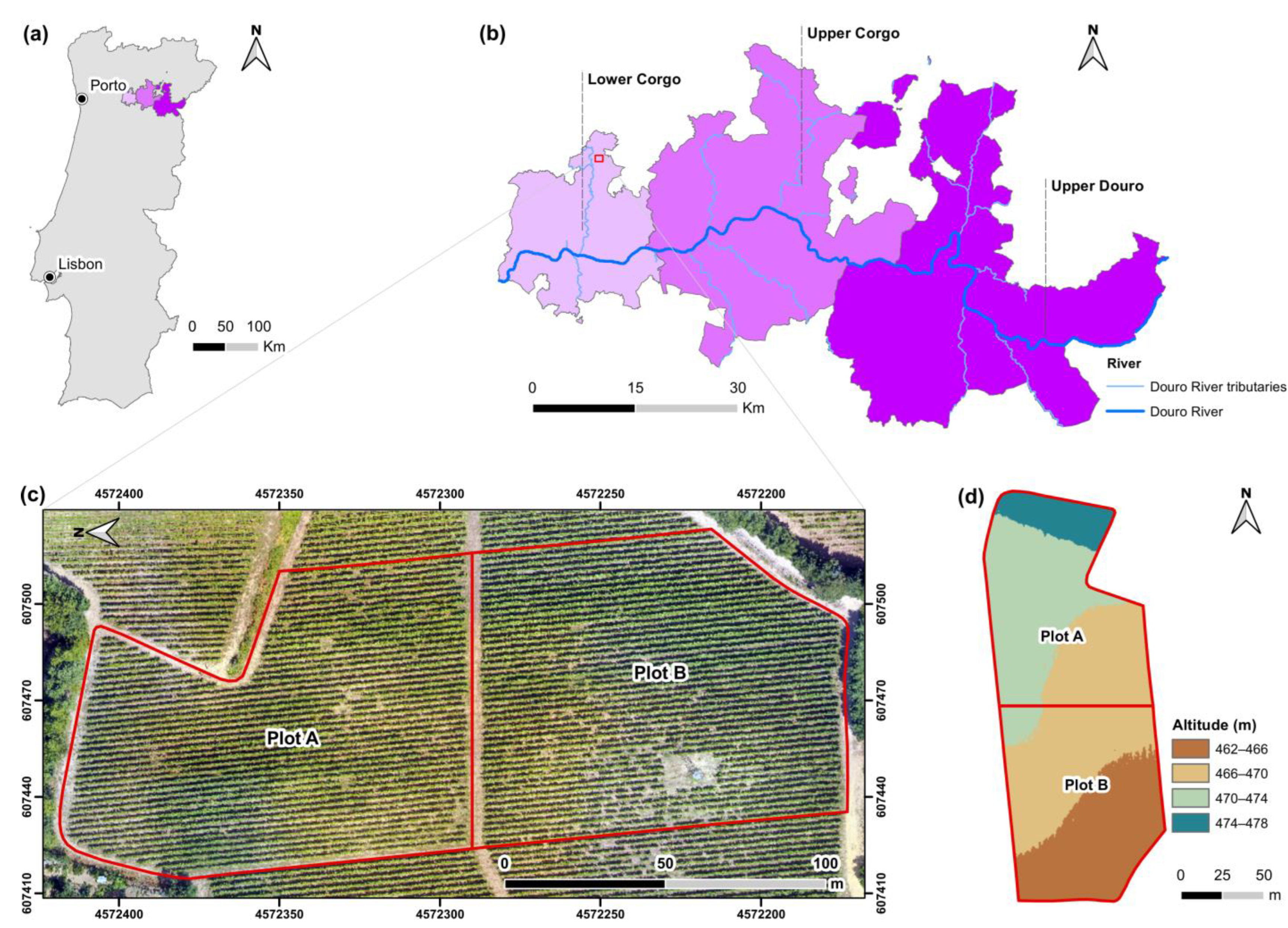
2.1. Study Area

The study was conducted in vineyards located in Vila Real, Portugal, within the Douro Demarcated Region (DDR) (Figure 1b), whose latitude and longitude positions range between 41°17′41.64″ N and 7°42′59.53″ W (World Geodetic System 1984-WGS84). The analyzed area covers a surface of about two hectares and is divided into two plots: Plot A (cv. Sousão) and Plot B (cv. Sauvignon blanc), each one with 1 ha of area (Figure 1c). The vine training system is Cordon Royat, adapted to a relatively low vegetative vigor. In each row, the grapevines are spaced by 1 m, with the distance between the rows at 2 m. A total of 45 rows with an N–S orientation are analyzed. Inter-row areas are composed of spontaneous vegetation, and grapevines are managed using mechanical interventions at least twice per season. In addition, it is a rainfed vineyard, with fertilization applied using foliar spraying, and with phytosanitary management operations taking place throughout the entire season.

The vineyard, predominantly facing south, is located on relatively plain ground, with Plot A at an altitude ranging from 467 to 478 m and Plot B at a lower altitude, between 462 and 471 m (Figure 1d). Due to the irregularity of the terrain morphology in terms of soil properties, the selected vineyard is characterized by vigor variation within and between the plots. During the studied period (April to September 2021), a total of 350 mm of precipitation was registered, corresponding to 35% of the total rainfall registered in 2021 (991 mm), along with 827 mm of evapotranspiration. Mean values for maximum, mean, and minimum air temperatures were 27.88 °C, 13.80 °C, and 2.77 °C, respectively. Monthly values of these variables are presented in Figure 2; the data were acquired using a weather station (iMETOS, Pessl Instruments GmbH, Weiz, Austria) located 200 m away from the study area. Higher air temperatures are observed in July, August, and September, while January, February, and December present higher precipitation values. In contrast, there is almost no precipitation in March, July, and August.

2.2. Remote-Sensed Data

The multispectral data used in this study are acquired from two different remote sensing platforms, Sentinel-2 and UAV, during the 2021 growing season, on six different dates between April and September (

Table 1. Acquisition dates of Sentinel-2 and unmanned aerial vehicle (UAV) data and the temporal difference between them for each analyzed period, the corresponding grapevine growth stages, and its BBCH codes [38] in each plot, where each growth stage corresponds to: 1—leaf development; 5—inflorescence emergence; 6—flowering; 7—development of fruits; and 8—ripening of berries.

Period	Acquisition Date	Data Source	Difference (Days)	Growth Stage	Bbch Code
April	30 April 2021	UAV	4	1 (both plots)	13 (plot A) 16 (plot B)
	4 May 2021	Sentinel-2
May	25 May 2021	UAV	4	5 (both plots)	55 (plot A) 57 (plot B)
	29 May 2021	Sentinel-2
June	11 June 2021	UAV	3	6 (both plots)	68 (plot A) 69 (plot B)
	8 June 2021	Sentinel-2
July	13 July 2021	UAV	0	7 (both plots)	71 (plot A) 73 (plot B)
	13 July 2021	Sentinel-2
August	4 August 2021	UAV	7	7 (plot A) 8 (plot B)	79 (plot A) 81 (plot B)
	28 July 2021	Sentinel-2
September	15 September 2021	UAV	6	8 (both plots)	85 (plot A) 89 (plot B)
	21 September 2021	Sentinel-2

), covering different grapevine vegetative stages.

2.2.1. Sentinel-2

The Sentinel-2 multispectral instrument (MSI) is capable of acquiring data in 13 parts of the electromagnetic spectrum, ranging from visible, NIR, to short wave infrared (SWIR), with spatial resolutions of 10 m, 20 m, and 60 m, a current revisit time of five days, and with an image ground coverage of 100 × 100 km per tile [39]. In this study, cloud-free Level-2A Sentinel-2 Bottom of Atmosphere (BOA) reflectance images were used. Level-2A processing includes scene classification and atmospheric correction applied to Level-1C ortho-image Top of Atmosphere (TOA) products [40]. In this study, only red and NIR bands (Bands 4 and 8, respectively) were used (for VI calculation). To avoid major divergences in the assessment of the vineyard vegetative status, Sentinel-2 data tiles in a date as close as possible to the period when the UAV flight mission took place were used.

2.2.2. Unmanned Aerial Vehicle

RGB and multispectral high-resolution aerial imagery acquisition were performed using the Phantom 4 (DJI, Shenzhen, China). RGB images were acquired with the native Phantom 4 camera, mounted on a 3-axis gimbal (FCC 3 camera model with 12.4 megapixels). Multispectral image acquisition was performed using the Parrot SEQUOIA sensor (Parrot SA, Paris, France) acquiring the green, red, red edge, and NIR bands, with a 1.2 MP resolution.

The UAV campaigns were carried out in different phenological phases defined in the Biologische Bundesanstalt, Bundessortenamt, und CHemische Industrie (BBCH) scale [38], from leaf development with three leaves unfolded (April), to the ripening of berries when grapes are ripe for harvest (September); more details provided in Table 1. Images were collected near solar noon to minimize shadow influences, in clear sky conditions, and with minimal wind effects, at a flight height of 50 m, with a frontal overlap of 80% and a 70% lateral overlap between the images.

The ground sampling distance (GSD) was approximately 0.02 m for the RGB and 0.05 m for the multispectral data. Furthermore, the radiometric calibration of the multispectral data is performed by taking a photograph of a reflectance panel provided by the manufacturer (Airinov, Paris, France) before each flight along with irradiance data from the sunlight sensor positioned on the top of the UAV. The irradiance and reflectance data allow for a reliable radiometric workflow to collect repeatable reflectance data over different flights, dates, and weather conditions.

2.3. Phenological Modeling

In order to generate reliable information on the behavior of the vineyard, the growing degree days (GDD) are calculated. Although other, more complex indices have been developed to assess the phenological stages, GDD remains as a simple comprehensive indicator that is used worldwide. Air temperature data are used to compute the correspondent GDD in the period from 1 January to 30 October 2021 according to the Winkler Equation [41,42,43], generally defined as in Equation (1):

$$GDD \left(t\right)={\displaystyle \sum }_{i=0}^t\left[\frac{T_{max}+T_{min}}{2}\right]-T_{base}$$

(1)

where t is the number of days from the starting date of GDD calculation (1 January), T_max is the daily maximum air temperature, T_min is the daily minimum air temperature, and T_base is the reference base temperature, below which, the process of interest does not progress. T_base varies among species and possibly cultivars and probably varies with the phase or growth process being considered [41]. For this study, a T_base value of 10 °C was considered, which corresponds to vegetative zero for grapevines [42]. The vineyard phenology defined based on the GDD corroborated the BBCH-scale [44], monitored weekly. To proceed with the analysis of the different grapevine phenological stages, six UAV and Satellite data acquisitions were carried out during the months of April to September 2021 (Figure 3). The data collected contemplated the main crop stages for grapevine, starting at leaf development (tree leaves unfolded), including inflorescence emergence, flowering, fruit development, and the ripening of the berries (berries ripe for harvest).

The GDD for 2021 in the study area along with the GDD values registered in the previous four years are presented in Figure 4; the heat unit for each period in the two remote sensing platforms is also provided. The most relevant phenological phases observed in the field were in line with other studies for cv. Sauvignon blanc [45] and for cv. Sousão [46].

2.4. Data Processing

UAV-based imagery acquired in each flight campaign is processed using the Pix4Dmapper Pro version 4.5.6 (Pix4D SA, Lausanne, Switzerland). This software uses structure from motion (SfM) algorithms to identify common points in the images. In the initial processing (step 1), the camera’s internal and external parameters are calibrated, and initial tie points are computed between the provided images, producing a sparse point cloud. In this stage, ground control points (GCPs) are established to ensure alignment between the data produced by the two sensors (RGB and multispectral) and the different periods. Six CPGs were distributed over the study area, of which four were assigned close to the corners of the area and two in the central region. In step 2, the dense point clouds are created and classified. In the last step, responsible for generating orthorectified raster products, the points within the dense point cloud are subjected to smoothing with noise filtering operations. Then, with the interpolation and orthorectification of the point clouds, the following outcomes are generated: (i) RGB orthophoto mosaic; (ii) digital terrain model (DTM); (iii) digital surface model (DSM); and (iv) vegetation indices, from the multispectral data.

To conduct a detailed analysis of each plot (Plot A and Plot B) from the radiometric information provided by the UAV-based multispectral data and then compare it with Sentinel-2 MSI data (10 m × 10 m), three scenarios using the UAV-based data were proposed: (i) considering all data, corresponding to pixels representing the whole vineyard features (including grapevines, inter-row vegetation, and bare soil); (ii) considering only grapevine canopy, which excludes all non-grapevine pixels; and (iii) considering inter-row areas, representing only pixels from vineyard inter-row areas (excluding all grapevine vegetation). Geospatial data are processed using QGIS geographic information system (version 3.22.8, Open Source Geospatial Foundation Project, http://qgis.osgeo.org (accessed on 9 October 2022)). Regarding the UAV data, first, a crop surface model (CSM) is computed from the difference between the DSM and DTM, as presented in Equation (2). The CSM is calculated from the data generated by the digital elevation models computed from the RGB imagery. The QGIS Raster Calculator tool is used to generate a CSM for each evaluated month (April to September).

$$CSM=DSM-DTM$$

(2)

From the CSM, two sets of six masks are produced to represent the grapevine canopy and the inter-row areas, respectively. The masks refer to pixels that have values at a given height. For the grapevine canopy, the masks are produced by removing all pixels referring to soil or inter-row vegetation, thus not belonging to the vineyards. Only pixels with height values greater than 0.2 m are selected for April and May, and 0.5 m from June onwards. On the hand, the inter-row masks are composed of non-grapevine pixels. These values are selected according to the height of the inter-row vegetation in each period. The masks are created as in Equation (3), where the sample pairs are differentiated by applying a certain inclusion criterion.

$$Mask=\frac{\left(CSM\alpha \times 1\right)}{\left[\left(CSM\alpha \times 1\right)+\left(CSM\beta \times 0\right)\right]}$$

(3)

where α corresponds to the height value of the data set to be filtered, and in front of it is assigned a sign that corresponds to the direction of the order of magnitude (e.g., >, ≥, < or ≤). β refers to the same value assigned to α, but it must be accompanied by the inverse of the magnitude sign. Pixel values of zero and one define the absence or presence of information at the end of the process, respectively. From these masks the three initially proposed scenarios are created by distinguishing grapevine canopy and inter-row elements. For each mask, the NDVI values are computed from the radiometric information provided by the UAV-based multispectral in Pix4Dmapper Pro, as in Equation (4). The assignment of NDVI values to the masks is performed directly using the QGIS raster calculator, with the multiplication of the binary values of the masks to those presented by NDVI in each period (April to September). A visual representation of the computed masks using an RGB orthophoto mosaic is presented in Figure 5.

$$NDVI=\frac{NIR-Red}{NIR+Red}$$

(4)

The pixel size used to produce the UAV-based NDVI is approximately 0.02 m (Figure 6a), which is very expressive, especially when compared to the coarser spatial resolution of Sentinel-2 MSI data (10 m). To allow a fair NDVI comparison between these two datasets, it is necessary to standardize the spatial resolution. This procedure is performed by using a grid projected over the two vineyard plots. The grid cell size is determined based on the Sentinel-2 pixel size and to match its location. Using the QGIS Zonal Statistics plugin, the mean NDVI values associated with the original pixels within each grid cell are calculated. The UAV-based NDVI values of each scenario hereinafter classified as all data, inter-row, and grapevine canopy in the different UAV flights and for the different Sentinel-2 acquisition dates are assigned to the same grid cell (Figure 6b). The last data processing step consists of selecting cells entirely within the boundaries of the study area, separating them by plot, resulting in 83 cells for Plot A and 80 cells for Plot B (Figure 6c). To compare the NDVI values between the plots, a similar procedure is implemented, assigning to each plot (1 ha) the mean NDVI value from each UAV-based approach and from the Sentinel-2 pixels within each plot.

The masks representing grapevines are used to determine their canopy area and volume and to evaluate the effect on the NDVI obtained by the satellite throughout the vegetative cycle. The total area of the grapevine canopy is obtained from the sum of the total number of pixels within each 10 × 10 m grid cell, multiplied by the area of the pixels (4 × 10⁻⁴ m²). The vine canopy volume is calculated by following a 2.5D approximation approach [47], which is based on the multiplication of the area of each pixel with the canopy height, from the CSM. The effect of the herbaceous vegetation of the inter-row areas in the NDVI value is also evaluated. For this purpose, a filter is applied to the NDVI values of the masks generated for the inter-row areas with the aim to consider only the pixels of vigorous plants with an NDVI value greater than 0.5 [48]. With this procedure, elements such as stones, exposed soil, and dry matter are not considered.

2.5. Data Analysis

In each flight campaign, the NDVI results obtained for the three UAV-based approaches (all vineyard data, grapevine canopy, and inter-row areas) are compared with the Sentinel-2 NDVI values using standard statistical approaches. The evaluation of the individual characteristics is performed for each plot. The comparison of NDVI values (mean, minimum, maximum, and standard deviation) is also performed for the three UAV-based approaches and Sentinel-2 NDVI data (hereinafter referred to as the satellite scenario). The statistical measures of the NDVI values generated for each scenario are displayed in the form of box diagrams.

A one-way ANOVA test is performed to determine if the independent variables (all data, inter-row, grapevine canopy, and satellite) present effects on the response variable (vigor). As the null hypothesis, it is considered that all scenarios are equal (H₀: x₁ = x₂ = … = x_n) against the alternative hypothesis, that at least one of the scenarios is different (H₁: x_i ≠ x_j = … = x_n, for at least one i, j, or n). To verify the statistical difference between the scenarios, Tukey’s test is applied at a 5% probability level [49]. The statistical relationship between the scenarios established from the UAV and Sentinel-2 data is described using the coefficient of determination (R²). Moreover, the mean NDVI value of each approach over time is analyzed in both vineyard plots using the different evaluated approaches.

3. Results

3.1. Data Characterization

The mean NDVI distribution for each plot over time for each approach is shown in Figure 7. In the different evaluated scenarios, the NDVI follows the development trend of the vineyard, with the lowest values registered in April and May. On the other hand, the maximum values are reached in July, with an overall decrease in August, followed by a slight increase in the harvest period (September). The difference between the average NDVI values for the different scenarios is lower in April and July, but slightly higher in May, June, August, and September. The lowest values are recorded in the inter-row regions, with a similar pattern to when using all data. Both plots show similar NDVI values in April, with a slight difference between the scenarios, which increased as the vineyard developed. In April, the vineyard is still in the leaf development stage (Figure 3). In this period, the inter-row was revealed to be the most expressive element, making the NDVI values closer to each other in all data approaches. As the grapevine canopy development proceeds, especially from August onwards, the effect of the inter-row areas is less noticeable. As happens for the UAV-based inter-row approach, the satellite (Sentinel-2) NDVI values are also slightly lower than all the UAV NDVI data, especially in April.

While Figure 7 presents the mean NDVI values obtained for each scenario, based on the original spatial resolution of each sensor, Figure 8 presents them from a different perspective, considering the Sentinel-2 spatial resolution, allowing a direct comparison between the datasets. It is possible to observe the statistical difference between the scenarios and to analyze the variability within and between the plots. In general, a similar trend is observed for both plots over the months, with lower NDVI values associated with the first months. The peak is reached in July, followed by a slight reduction the following month, and a new increase in September. UAV-based grapevine canopy was the scenario with the highest NDVI values, especially in Plot B (Figure 8b). A lower interquartile range is also evidenced for the grapevine canopy dataset, with the median showing a tendency towards the highest NDVI values.

In April, the grapevines are at the leaf development stage, and thus have a less significant contribution regarding the soil cover area. Given this conjuncture, except for the satellite dataset, no statistical differences are observed in Plot A between the different scenarios (p ≥ 0.98). For Plot B, on the other hand, using only the grapevine canopy differs statistically from the other approaches, not only in April but in every month. It is worth noting that all data and inter-row scenarios are not statistically different (p = 0.23), but both are different from the satellite-based NDVI. The lowest NDVI value associated with the satellite dataset is observed in April. In May, with inflorescence emergence, all scenarios statistically differ, with the highest NDVI values recorded for grapevine canopy, satellite, all data, and inter-row, respectively. Even with the continuous development of the vine canopy, in this stage, the inter-row areas remain the most representative element in the vine-growing area. The low NDVI values associated with the inter-row areas may have influenced the value of all data and satellite, which represent the whole surface of the vine-growing area. In the flowering period (June), a reduction in the difference between the average NDVI values of the grapevine canopy and all data is observed. In both plots, the grapevine canopy differs from the other scenarios. In Plot A it is possible to observe that there is no difference between all data and satellite (p = 0.61); nevertheless, the NDVI is higher than the one presented by the inter-row. Meanwhile, in Plot B, the lowest values are associated with the inter-row and the satellite (p = 0.77). In July, during the development of fruits, the grapevine canopy values obtained in Plot A are similar to those observed for all data (p = 0.05), the latter not statistically different from the inter-row (p = 0.06). Regarding Plot B, the scenario with grapevine canopy is the most prominent, followed by all data and inter-row, which are not statistically different (p = 0.05). In both plots, satellite is the scenario with the lowest NDVI value associated.

An overall reduction in the mean NDVI value is verified in August. Nevertheless, vegetation management carried out in the vineyard (between July and August), such as pruning and the cleaning of the inter-row certainly contributed to this NDVI reduction. The decrease in vigor has a strong effect on the inter-row, with a direct effect on the surface of the vine growing area, which is evaluated by all data and satellite scenarios. This fact can be corroborated by the data obtained for Plot B, where the values observed in the inter-row do not present statistical differences from those obtained by the satellite (p = 0.98). Similar behavior is observed in June. In September (ripening of berries), the NDVI values increased again, and the difference between the grapevine canopy and the other scenarios remains, especially if compared to the inter-row and satellite scenarios, which do not differ from each other, both in Plot A (p = 0.99) and in Plot B (p = 0.20).

A similar analysis was performed regarding the grapevine canopy area and volume computed from the UAV-based data (Figure 9). The same general trend in the NDVI average values is detected in all scenarios. The grapevine canopy area is not very expressive in the first three months, the period where vegetative growth occurs. The same happens with grapevine canopy volume, which is directly affected by its area and height. In May, there is a reduction of 51% in Plot A’s inter-row area, and 62% in Plot B. The most relevant values in terms of grapevine canopy area and volume are obtained in July, the period that demonstrated the greatest vigor (Figure 8). The pruning operations, carried out between July and August, are responsible for a reduction of 18% of the grapevine canopy area and 19% of the volume in both plots. Similar behavior is detected for the inter-row vegetation after being submitted to vegetation management operations. A reduction of 19% in Plot A and 14% in Plot B can be observed. From August to September, there is a tendency towards a balance between the area occupied by the grapevine canopy and by the inter-row herbaceous vegetation.

These results clearly show that the grapevine canopy area observed in Plot B is higher than in Plot A, throughout the period evaluated, especially in April, with a difference of 8%. The reducing trend continued in the remaining months, although it was more attenuated over time, reducing 6% in May, 4% in June, 3% in July and August, and less than 1% in September. The difference is greater in the first months, followed by a gradual decrease with the growth of the vegetative organs of the grapevine. The grapevine canopy volume in Plot B is greater than in Plot A between the months of April and June. The difference is attenuated in July, after which, there is an opposite effect since the vine canopy volume of Plot B is exceeded by Plot A and reaches a difference of 82.62 m³ha⁻¹, in September. It is also observed that from May to July, Plot A presents a greater amount of inter-row herbaceous vegetation when compared to Plot B. On the other hand, Plot B exhibits a greater grapevine canopy volume and occupies a larger area.

3.2. Data Correlation

The linear correlation between the predictor variables from the UAV-based data (all data, inter-row, and grapevine canopy) with the response variable from Sentinel-2 (satellite) is presented in Figure 10. The degree of linear adjustment for the period from April to September is higher in Plot A, especially for grapevine canopy (R² = 0.77), which outperformed the all data (R² = 0.72) and inter-row (R² = 0.63) approaches. With regard to Plot B, the all data approach is more expressive, with the ability to explain 66% of the variance of the NDVI values obtained with the linear model, followed by the inter-row (R² = 0.59) and grapevine canopy (R² = 0.58) approaches. Through the combined analysis of Plot A and Plot B, all data, inter-row, and grapevine canopy are not sufficiently able to explain all the existing variation in the response variable. However, it should be noted that the linear models established for the different scenarios and plots explain at least 58% of the variance of the satellite NDVI values, obtained over the six-month period starting in April 2021.

For the study period (six months), the grapevine canopy NDVI values are sufficiently able to explain much of the variation over the satellite-based data. However, the same cannot be said of the individualized analysis for each month.

Table 2. Coefficient of determination (R²) obtained from the linear correlation of the predictor variables (derived from the unmanned aerial vehicle—UAV—inter-row, grapevine canopy, and all data approaches) with the normalized difference vegetation index (NDVI) values of the satellite (Sentinel-2): when using the NDVI values; when using the vegetation cover area associated with the grapevine canopy, herbaceous vegetation in inter-row areas (NDVI > 0.5), and all data, that represents the sum of the vegetation cover associated with the two previous categories; and the correlation with grapevine volume, ns: non-significant.

Plot	Scenario	April	May	June	July	August	September
Normalized difference vegetation index
A	Inter-row	0.78	0.88	0.66	0.66	0.30	0.81
	Grapevine canopy	0.17	0.57	0.59	0.63	0.41	0.71
	All data	0.78	0.87	0.63	0.66	0.49	0.84
B	Inter-row	0.73	0.74	0.78	0.79	0.24	0.92
	Grapevine canopy	0.23	0.62	0.61	0.24	0.02	0.78
	All data	0.79	0.87	0.77	0.75	0.55	0.93
Vegetation cover area
A	Inter-row	0.69	0.80	0.67	0.15	0.05	0.10
	Grapevine canopy	0.16	ns	0.06	0.19	0.47	0.69
	All data	0.56	0.84	0.61	0.14	0.42	0.42
B	Inter-row	0.31	0.55	0.78	0.25	0.02	0.12
	Grapevine canopy	0.35	0.30	0.11	0.29	0.68	0.77
	All data	0.70	0.81	0.80	0.28	0.52	0.68
Grapevine volume
A	Grapevine canopy	0.19	0.01	0.08	0.26	0.42	0.73
B	Grapevine canopy	0.29	0.22	0.27	0.50	0.72	0.85

shows that all data and inter-row scenarios can better explain the variation in the satellite-based NDVI values, compared to the grapevine canopy. In the first months of vegetative development, the grapevine leaf area is quite reduced and is limited to the region around the plant’s trunk. The plant species that can be found under grapevines and especially in the inter-row areas, in April, have a great impact influencing the NDVI values, as it is the most representative element for the period. From May onwards, grapevines gain more biomass, and the development of the shoots allows the plant to expand its leaf area. This is when the grapevines start to gain more visibility and influence the global vigor of the vineyard plot. However, the vegetative grapevine growth is conditioned in the planting row and does not cover the whole plot surface. On the other hand, the inter-rows areas maintain the behavior throughout the entire vegetative cycle of the vineyard. However, when the grapevines show low vegetative expression, mainly at the leaf development stage (April) and immediately after the grapevine interventions (May), the inter-rows approach shows increased behavior (Figure 9). In July, the grapevine canopy reaches the peak of its development, so its contribution in terms of vigor is expected to culminate in a higher correlation with the Sentinel-2 NDVI values. Indeed, it presents an increase in the correlation of the grapevine canopy in Plot A. However, the same is not observed in Plot B, where the correlation of the inter-row values is higher than the grapevine canopy values and enables a better explanation of the Sentinel-2 NDVI values. In August, there is a lower correlation in all scenarios. In the following month, both the inter-row and grapevine canopy values show a good correlation with Sentinel-2 but are outperformed by the all data approach.

From the analysis of the NDVI values of the different UAV-based scenarios with Sentinel-2 NDVI (Table 2), all data can better explain the Sentinel-2 NDVI values since it considers the whole grapevine growing area. In this case, the difference in resolution does not significantly affect the global behavior. The inter-row approach is a slice of the all data approach, but one that exerts more influence on the Sentinel-2 NDVI than the grapevine canopy itself. The grapevine canopy area and the inter-row vegetation area seem to influence in some way the NDVI values computed by the satellite data.

To better understand this relationship, a correlation analysis is performed between the satellite NDVI values and the respective area associated with the inter-row vegetation, the grapevine canopy, and all data, which is the result of the sum of the two previous. The findings presented in Table 2 indicate that the area of the scenarios exerts a certain effect on the NDVI value of the satellite. It can be also observed that the grapevine canopy area presents a certain level of correlation with the satellite in the grapevine ripening period, which occurred in August for Plot B and in September for Plot A. This is the opposite scenario of what is observed for the inter-row vegetation area, which shows a high correlation in the first months (April, May, and June), precisely when the vine has less canopy area and volume. In the present study, the grapevine canopy area occupies 12% to 49% of the crop area in Plot A, and 20% to 53% in Plot B. In both plots, April represents the month with the lowest coverage, and July represents the peak.

Table 2 also reveals that the area of each scenario is not able to fully explain the variation in the satellite NDVI values for the periods corresponding to the grapevine’s growth and maturation. In July, for example, the grapevine canopy area and volume are more expressive than in any other month (Figure 9), but a low correlation with the satellite NDVI is obtained in both plots. It is possible to observe that grapevine vigor is a response to the growth of the vegetative organs, which is difficult to detect in the satellite data at the beginning of the vegetative cycle. It is also found that the canopy area can influence this process, especially during the ripening season (August to September), motivated by the reduced variability and the superiority of the grapevine canopy area in relation to other types of vegetation present in inter-row areas. To corroborate this result, the relationship between the grapevine canopy volume and the satellite NDVI value is also analyzed. The values found are presented in Table 2, where it is possible to observe that from July onwards (Plot B) and from August onwards (Plot A), the grapevine canopy volume can exert an effect on the satellite NDVI value. It is also worth noting that the correlation is higher for Plot B, especially before September. In this period, Plot B presents the largest grapevine canopy area and volume, being only surpassed by Plot A in September, but only concerning the volume (Figure 9).

4. Discussion

4.1. Multi-Temporal Analysis of the Different Approaches

The multi-temporal vineyard monitoring performed in this study provided interesting results in several aspects. The changes that occur in the phenological stages are well expressed in the GDD accumulation (Figure 4) and have a close relationship with NDVI values, as already remarked by other authors [50]. Typically, the NDVI and GDD curves are similar to each other and follow the annual grapevine biological cycle [51]. The same behavior is also observed in this study, both in the Sentinel-2 and UAV datasets. From the phenological modeling (Figure 4), the GDD accumulation in 2021 is higher in the first four months of the year compared to the average of the previous four years. The knowledge of the phenological phases is decisive in establishing a robust approach around the NDVI values computed from satellite and UAV multispectral imagery. The multi-temporal analysis conducted for the different approaches (Figure 7 and Figure 8) clearly reveals that there are different behaviors in terms of vine development over time. As elucidated in Figure 2, the period between April and June was favored in terms of precipitation, which certainly contributed to the development of spontaneous vegetation, which happened earlier than grapevines [52]. Nevertheless, the reduced grapevine canopy area and volume allowed for greater sunlight exposure in the inter-row areas, which mainly benefited the heliophyte herbaceous plants (Figure 9) [51]. Due to the absence of vine canopy cover in the first months of the year, the spontaneous vegetation in the inter-row areas is the only element capable of expressing the plot’s vegetative vigor. Such information is of great agronomic utility. In the northern hemisphere, April is the ideal period to conduct vineyard soil fertilization, by applying higher rates in places where the vegetative vigor is lower [27]. In addition, as the inter-row vegetation usually undergoes at least one intervention a year, the information can also be used to plan the future maintenance activities of spontaneous vegetation, such as mowing or tillage, which are intended to reduce water competition from permanent plants and also to minimize the risk of vineyard frost damage [53].

The higher mean NDVI values from the UAV multispectral data at the grapevine canopy level are notable, which differed statistically from the other scenarios in almost the entire grapevine canopy growth period (Figure 8). Therefore, it can be stated that the vineyard plot segmentation approach, used to distinguish pure grapevine canopy pixels from the other vineyard elements [37], proves to be an appropriate way to obtain the vigor associated with the grapevine canopy. In fact, the exclusive use of grapevine vigor is the only way to avoid biased evaluations, especially for cordon training, where the inter-row area can be covered with grass and other crops, subject to anthropic interventions, such as pest and disease control or soil cleaning [31].

As NDVI is strongly influenced by vineyard surface structure, canopy architecture, and leaf orientation [54], any change occurring in the vineyard area has a direct impact on the plot’s vigor. However, many of the nuances that happened in the vineyard plots could not be noticeable from the Sentinel-2 data (Table 2). For example, the NDVI value decreased for all data and inter-row, which occurred in May, right after the cutting of spontaneous vegetation (Figure 8), and the slight reduction in the grapevine canopy area in June (Figure 9), subsequent to the orientation and steering activity of the shoots, were both detected only in the UAV dataset. The coarser spatial resolution of the Sentinel-2 data is responsible for the high NDVI variability observed (Figure 8). For a given pixel, a higher proportion of unwanted elements than just the area occupied by the grapevine canopy cause this to occur in the satellite images [23] since the spectral values of the images are subject to the boundary effect when pixels near the boundary region of the area of interest can be contaminated by adjacent elements, such as paths, open fields, and other vegetation typologies, which have the ability to reduce or increase the spectral value of the pixels [23,30]. The spatial resolution of Sentinel-2 images can be a real obstacle since it prevents the use of vegetation filtering methodologies [7] such as the one used in this study. On the other hand, Sentinel-2 multi-temporal data are able to detect important vineyard interventions, such as pruning, which is performed to control vigor, stimulate the development of secondary shoots, promote productive activity [27], and increase plot uniformity [55]. The ability of the satellite time-series data to detect these transformations is obtained from the correlation between the satellite NDVI and the scenarios produced by the UAV (Figure 10). The consistency between the information provided by the two platforms is confirmed by the R² values, which are higher than 0.6 for more than 78% of the comparison performed, and never lower than 0.58. Khaliq et al. [31] studied the cv. Nebbiolo in Piedmont (northwestern Italy), and the values obtained from the Pearson correlation (r) between Sentinel-2 and similar UAV approaches to the ones used in this study were also expressive, higher than 0.55. The potential of using Sentinel-2 images to characterize vigor with NDVI is also reinforced by Devaux et al. [30].

The peak of vegetative development is reached in July (Figure 8 and Figure 9), being consistent with what is reported in grapevine growth in the northern hemisphere [23,30,31,56,57]. However, this is not a rule since it can vary according to the genetic vineyard characteristics and the climatic conditions of the winegrowing year [27]. Despite the increase in vigor associated with the grapevine canopy, in July, lower correlations were recorded between the grapevine canopy area and Sentinel-2 NDVI. It is believed that the canopy area growth may have contributed to the increased vigor variability in the plots. In this period, the grapevine leaves reach their full development [52], with a larger leaf area, and secondary shoots started to emerge from the primary shoots with young leaves, those are consumers of photo-assimilates with the ability to influence the reflectance of the grapevine canopy and, consequently, the NDVI value. Such differences in the grapevine canopy can be detected by the UAV-based data, given its spatial resolution [7,36], which would explain the low correlation between the grapevine canopy area and Sentinel-2 NDVI, due to its coarser resolution.

Between July and August, there was little influence of rainwater on the soil (Figure 2), with these being the months with the greatest hydric need. The overall reduction in the NDVI values in the vineyard recorded in August is related to the rise in average temperature values, the absence of precipitation, soil moisture decrease, and the absence of water supply to the plants [27,52]. According to Puig-Sirera et al. [54], soil water deficit in the veraison period (during August) can be responsible for the reduced photosynthetic activity and, consequently, vegetative vigor reduction. The leaf area reduction is an evolutionary strategy of vines to minimize water loss. In fact, subareas with more vigorous vines tend to experience more significant levels of water stress, which can often compromise both yield and production quality [58]. Even with the water restrictions, the grapevine canopy is able to maintain vigor at higher levels than herbaceous vegetation in between the rows, as observed in Figure 8. This result shows that grapevine vigor is less affected by dry and hot conditions than herbaceous vegetation [52]. In this case, even if there was variability in the same plant or row, the grapevine canopy area would eventually fulfill the row voids [59], and along with inexistent inter-row vegetation, it becomes the component with the greatest contribution to express the actual vineyard plot vigor detected by Sentinel-2 data.

The dry conditions in conjunction with anthropic interventions in the crop area between the months of July and August caused an immediate effect on the vegetation in the inter-row areas (Figure 9). Pruning activities reduced the overall vigor of the two analyzed plots and their canopy area, which became less than 43% of the vineyard plot. As a consequence, the exposure between the rows increases. With this, it is expected that the area between the rows would exert more influence on the Sentinel-2 NDVI value, given its greater representativeness, which did not immediately occur. The vigor reduction (Figure 8) and the decrease in the inter-row herbaceous vegetation area to less than 39% of the plot (Figure 9) caused an increase in the heterogeneity of the environment, seen by the eminence of a mixture of elements (e.g., exposed soil, stone, dry mass, etc.), which represented 18% of the area. Probably the higher inter-row variability detected through the UAV multispectral data was not captured by the satellite, which would explain the low correlation between the satellite NDVI value with the different scenarios.

The grapevine canopy area and volume gained more relevance in September, just after the veraison phase, when the increase in the correlation between the grapevine canopy and the Sentinel-2 NDVI occurred (Table 2). In this period, the vineyard is fully developed and no major transformations occur, so the spatial patterns of the NDVI are more stable [54]. However, due to the lower resolution of the Sentinel-2 images, it is expected that the satellite values would be underestimated compared to the resulting UAV scenarios [29]. Nevertheless, this trend was not always observed (Figure 8). In May, the Sentinel-2 NDVI values for both plots exceed the values found for inter-row and all data from the UAV-based NDVI, while in June and August, the inter-row NDVI of Plot A is also lower than that recorded by the Sentinel-2. It is likely that the reduction in the inter-row NDVI values is the result of the interventions that happened at the plot level, such as cutting the herbaceous vegetation.

The coefficients of determination produced from May to September are in line with the literature [31,37,55]. Among the scenarios evaluated, the grapevine canopy is the one that is least related to the Sentinel-2 NDVI value, corroborating what has been obtained by other authors [55]. The R² values of the grapevine canopy ranged between 0.17 and 0.71 for Plot A and between 0.02 and 0.78 for Plot B (Table 2). The range between the values is significant when compared to the R² obtained by Pastonchi et al. [55] in vineyard plots of the cv. Sangiovese in Tuscany (Italy), which ranged between 0.53 and 0.80, as well as Khaliq et al. [31], who established comparisons by means of the correlation coefficient (r) and obtained values between 0.28 and 0.61. However, the time interval adopted in this study is six consecutive months, starting in April, while Khaliq et al. [31] concentrated their observations in the months of May, June, August, and September, and Pastonchi et al. [55] in June and August of 2017 and 2018, as well as August and September of 2019. For the approach considering only the inter-row areas in the UAV-based data, the R² of Plot A varied between 0.30 and 0.88, and in the case of Plot B, between 0.24 and 0.92. With the exception of August, the other months evaluated in this study presented higher R² values, greater than 0.66. Khaliq et al. [31] obtained a similar behavior; with the exception of a certain plot, all r values were greater than 0.50. Finally, when using all UAV-based data the results are the most congruent and have the least discrepancy between the correlations obtained, both in Plot A (0.49 to 0.87) and Plot B (0.55 to 0.93). This result is analogous to that obtained by Pastonchi et al. [55], with an R² between 0.59 and 0.80, as well as Khaliq et al. [31], with an r between 0.55 and 0.72. When correlating all data from both approaches, May and September presented the highest R², with values between 0.87 and 0.93, which far exceed what is obtained by Matese et al. [37] for two cv. Cabernet Sauvignon vineyard plots in Italy, who found r values in the comparison of UAV and the RapidEye satellite data ranging between 0.29 and 0.80.

The positive correlations obtained in this study are in line with the ones obtained in other studies [31,55]. However, some differences between the maximum and minimum values are observed. In May, the highest correlations between the NDVI values are obtained for the inter-row and all data approaches in both plots. In Plot A, R² = 0.88 is obtained when observing only inter-row vegetation and 0.87 when considering the whole UAV vineyard NDVI data, while in Plot B, the value was 0.74 and 0.87 for inter-row and all data, respectively. For the same period, Khaliq et al. [31] found r values ranging from 0.52 to 0.59 for inter-row areas and 0.60 to 0.64 when considering all data. As shown in Table 2, the R² values for the grapevine canopy are greater than 0.50 in 67% of the evaluated months for Plot A and 50% in the case of Plot B. Unlike Khaliq et al. [31], where only 17% of the r values recorded in three monitored plots over four months are greater than 0.50. The superiority of the determination coefficients observed in this study, compared to that described by Khaliq et al. [31], may result from differences related to the methodology employed in the analysis, the vineyard management, and the vigor of the plot itself. Particularly, the inter-row, which sometimes presents itself as the element that has the largest area in the plot, as previously discussed, among the elements existing in the vineyard plot, is the one that best correlates with Sentinel-2 data. As inter-row is a greater contributor, it tends to be detected more easily by Sentinel-2; the grapevine canopy vigor ends up being underestimated in almost the entire active growth period.

When comparing data from both vineyard plots, it was possible to observe the phenological differences between the red and white varieties analyzed in this study. Plot B showed slightly higher NDVI values than Plot A when considering only grapevine canopy during the entire study period (Figure 7), despite both plots being subjected to the same agronomic practices and sharing the same climatic conditions and soil type. Comparetti and Silva [27] verified that the difference in vigor for cvs. Nero d’Avola and Syrah in the Sicily region (Italy) could be explained by the genetic characteristics of each cultivar. In fact, in this study, cv. Sousão (Plot A) is a red grape variety, while cv. Sauvignon Blanc (Plot B) is a white variety, and usually, the white varieties have an earlier maturation than the red ones [60], and this is observed in the GDD analysis, which revealed that cv. Sauvignon Blanc needs less GDD than cv. Sousão to advance in the phenological phases [46,61]. This can help to explain the higher values of the grapevine canopy area and volume for Plot B in the first months of the year (Figure 9), as well as the earlier maturation of cv. Sauvignon Blanc, observed by the progressive reduction in its growth and the progressive increase in the canopy volume of cv. Sousão.

4.2. Benefits of Synergistic or Individual Use of Sentinel-2 and UAV Multispectral Data

Through the results obtained in this study and supported by other studies [27,29,30,31,37,55], it is demonstrated that both Sentinel-2 and UAV multispectral data are able to determine the temporal vineyard variability along the phenological stages of the grapevine vegetative development. In this sense, when considering the absence or minimal presence of grapevine vegetation, during senescence (after the end of leaf fall), sprouting, and leaf development, high correlations are obtained in Table 2. Therefore, Sentinel-2 MSI data can be applied to monitor the overall vineyard vigor. This can be achieved by using the spectral information from spontaneous vegetation in the inter-row areas within the vineyard, contributing to the management and operationalization of interventions at the plot level and correcting potential soil nutrient deficiencies. During the fruit development and ripening stages, Sentinel-2 also proved to be effective. This is due to the spatial structure of the vegetation being more homogeneous, a condition that favors an adequate representation of grapevines [37], making this period also suitable for being assessed by Sentinel-2 data. These conclusions are of paramount importance, as they allow the use of broad spatial coverage data with no significant coats (data are freely distributed). This makes Sentinel-2 MSI data the most suitable tool for monitoring vineyard spatial variability at a regional scale [30]. It is also possible to achieve similar coverage areas through UAVs, achieving higher or similar temporal resolutions, but it is more time-consuming, with significantly increased costs for larger areas [37], requiring human resources (at least two), several trips and working days, or by using several UAVs, batteries, and hardware for data storage and processing [62,63].

Sentinel-2 MSI data can also be used by winegrowers that have knowledge of field interventions to understand the overall changes in vineyard plots across time. This is indeed true, as the main phenological changes and transformations caused by anthropic activities, such as pruning, are well detected using Sentinel-2 data. However, statistical analysis indicated that UAV remote sensed data provides higher accuracy in estimating grapevine-level characteristics when compared to Sentinel-2 estimations, especially in periods when plot-level interventions were performed and at the time of greatest grapevine vegetative growth when greater canopy variability occurred. Due to the lower spatial resolution of Sentinel-2 imagery, it is almost impossible to separate soil effects from crop effects for any given pixel acquired on a vineyard plot with representativeness of less than 25% of the total area [7]. However, when using UAV-based data it is perfectly possible to distinguish the grapevine canopy from other elements.

UAV-based data can be used throughout the whole vegetative cycle [56] but can be discarded in the early development stages. In fact, UAVs can also be used with different sensors, which leads to new opportunities for specific applications. If vegetation needs to be mapped or classified, RGB data can be used [64]; this type of analysis can be conducted to obtain grapevine and inter-row vegetation areas [56]. In fact, it is possible to monitor interventions performed in the vineyards, but not the effects on their vigor, which is achieved in this study. Multispectral data enable obtaining vineyard biophysical parameters, enabling vigor mapping excluding non-grapevine areas [48,57], a process that cannot be performed using Sentinel-2 MSI data. The possibility to map inter-row vegetation within the vineyard can be used for discriminating invasive species among other cover crops [65]. Moreover, given the high spatial resolution of UAV-based data, it is possible to extract individual grapevine structural and biophysical parameters, which can be of extreme importance to help in vineyard analysis [59,66,67]. In PV management, plant-scale analysis can also be used to automatically detect and count missing grapevines for disease detection [68,69] and water stress monitoring [70,71].

5. Conclusions

The present study explores an approach based on cost-effective remote sensing that may bring promising results, contributing to the development of PV and the improvement of the production system, ensuring uniform and stable production in terms of quality, as well as the possibility of increasing profitability. It is based on the use of medium-resolution imagery, which is generally under-utilized compared to high-resolution UAV imagery, but which can contribute to the monitoring of parameters related to grapevine integrity and management to better monitor plant growth over time and assess their performance. It is verified that the Sentinel-2 MSI data and the information derived from the UAV-based data are both relevant for vigor management and to detect vineyard variability. An ideal solution for precision viticulture is the combined use of both remote sensing platforms. For obtaining general vegetation information on a given vineyard plot, Sentinel-2 can be considered the most economically advantageous option. However, if the purpose is to segment the elements on the ground surface using applied filtering techniques and pure pixel spectral data, as well as to define localized operations at the plant level, then UAV-based data are more suitable.

The analysis performed to compare the ability of Sentinel-2 and UAVs to determine the phenological phases of the vineyard reveals that the average NDVI values were very similar for both remote sensing platforms (when converted to the same resolution). The main differences were observed right after the agronomic interventions at the plot level. The vineyard plot segmentation shows that inter-row elements are sometimes the most influential on Sentinel-2’s NDVI. It is also found that the effect of the inter-row vegetation in the Sentinel-2 NDVI is smaller when inter-row variability is reduced, which increases Sentinel-2’s ability to detect grapevine canopy vigor. To improve the use of Sentinel-2 in vineyard plots conducted in the cordon, reducing the heterogeneity between rows seems to be an interesting option. However, more experiences are needed to confirm and corroborate these findings. Further research should be conducted to assess different arrangements between rows, such as types of cover plants, soil management practices, and soil cover with aggregate.

References

1. Khosla, R. Precision Agriculture: Challenges and Opportunities in a Flat World. In Proceedings of the 2010 19th World Congress of Soil Science, Soil Solutions for a Changing World, Brisbane, Australia, 1–6 August 2010; pp. 26–28. [Google Scholar]
2. Pierce, F.J.; Robert, P.C.; Mangold, G. Site Specific Management: The Pros, the Cons, and the Realities. In Proceedings of the Integrated Crop Management Conference, Ames, IA, USA, 30 November–1 December 1994; p. 11934214. [Google Scholar]
3. Santesteban, L.G. Precision Viticulture and Advanced Analytics. A Short Review. Food Chem. 2019, 279, 58–62. [Google Scholar] [CrossRef] [PubMed]
4. Matese, A.; Di Gennaro, S.F. Technology in Precision Viticulture: A State of the Art Review. Int. J. Wine Res. 2015, 69. [Google Scholar] [CrossRef] [Green Version]
5. Manson, S.M.; Bonsal, D.B.; Kernik, M.; Lambin, E.F. Geographic Information Systems and Remote Sensing. In International Encyclopedia of the Social & Behavioral Sciences, 2nd ed.; Wright, J.D., Ed.; Elsevier: Oxford, UK, 2015; pp. 64–68. ISBN 978-0-08-097087-5. [Google Scholar]
6. Viscarra Rossel, R.A.; Adamchuk, V.I.; Sudduth, K.A.; McKenzie, N.J.; Lobsey, C. Proximal Soil Sensing: An Effective Approach for Soil Measurements in Space and Time. Adv. Agron. 2011, 113, 243–291. [Google Scholar]
7. Brook, A.; De Micco, V.; Battipaglia, G.; Erbaggio, A.; Ludeno, G.; Catapano, I.; Bonfante, A. A Smart Multiple Spatial and Temporal Resolution System to Support Precision Agriculture from Satellite Images: Proof of Concept on Aglianico Vineyard. Remote Sens. Environ. 2020, 240, 111679. [Google Scholar] [CrossRef]
8. Hall, A.; Lamb, D.W.; Holzapfel, B.; Louis, J. Optical Remote Sensing Applications in Viticulture—A Review. Aust. J. Grape Wine Res. 2002, 8, 36–47. [Google Scholar] [CrossRef]
9. Gatti, M.; Dosso, P.; Maurino, M.; Merli, M.C.; Bernizzoni, F.; José Pirez, F.; Platè, B.; Bertuzzi, G.C.; Poni, S. MECS-VINE®: A New Proximal Sensor for Segmented Mapping of Vigor and Yield Parameters on Vineyard Rows. Sensors 2016, 16, 2009. [Google Scholar] [CrossRef] [Green Version]
10. Remote Sensing Handbook for Tropical Coastal Management. Green, E.P., Edwards, A.J., Eds.; Coastal Management Sourcebooks; Unesco Pub: Paris, France, 2000; ISBN 978-92-3-103736-8. [Google Scholar]
11. Alvarez-Vanhard, E.; Corpetti, T.; Houet, T. UAV & Satellite Synergies for Optical Remote Sensing Applications: A Literature Review. Sci. Remote Sens. 2021, 3, 100019. [Google Scholar] [CrossRef]
12. Mulla, D.J. Twenty Five Years of Remote Sensing in Precision Agriculture: Key Advances and Remaining Knowledge Gaps|Elsevier Enhanced Reader. Biosyst. Eng. 2013, 114, 358–371. [Google Scholar] [CrossRef]
13. Sishodia, R.P.; Ray, R.L.; Singh, S.K. Applications of Remote Sensing in Precision Agriculture: A Review. Remote Sens. 2020, 12, 3136. [Google Scholar] [CrossRef]
14. Yang, G.; Liu, J.; Zhao, C.; Li, Z.; Huang, Y.; Yu, H.; Xu, B.; Yang, X.; Zhu, D.; Zhang, X.; et al. Unmanned Aerial Vehicle Remote Sensing for Field-Based Crop Phenotyping: Current Status and Perspectives. Front. Plant Sci. 2017, 8, 1111. [Google Scholar] [CrossRef] [Green Version]
15. Katsigiannis, P.; Galanis, G.; Dimitrakos, A.; Tsakiridis, N.; Kalopesas, C.; Alexandridis, T.; Chouzouri, A.; Patakas, A.; Zalidis, G. Fusion of Spatio-Temporal UAV and Proximal Sensing Data for an Agricultural Decision Support System. In Proceedings of the Fourth International Conference on Remote Sensing and Geoinformation of the Environment, Paphos, Cyprus, 12 August 2016; Themistocleous, K., Hadjimitsis, D.G., Michaelides, S., Papadavid, G., Eds.; Volume 9688. [Google Scholar]
16. Gasmi, A.; Masse, A.; Ducrot, D.; Zouari, H. Télédétection et photogrammétrie pour l’étude de la dynamique de l’occupation du sol dans le bassin versant de l’oued Chiba (Cap-Bon, Tunisie). Rev. Fr. Photogrammétrie Télédétection 2017, 43–51. [Google Scholar] [CrossRef]
17. Romero, M.; Luo, Y.; Su, B.; Fuentes, S. Vineyard Water Status Estimation Using Multispectral Imagery from an UAV Platform and Machine Learning Algorithms for Irrigation Scheduling Management. Comput. Electron. Agric. 2018, 147, 109–117. [Google Scholar] [CrossRef]
18. Hatfield, J.L.; Prueger, J.H.; Sauer, T.J.; Dold, C.; O’Brien, P.; Wacha, K. Applications of Vegetative Indices from Remote Sensing to Agriculture: Past and Future. Inventions 2019, 4, 71. [Google Scholar] [CrossRef] [Green Version]
19. Giovos, R.; Tassopoulos, D.; Kalivas, D.; Lougkos, N.; Priovolou, A. Remote Sensing Vegetation Indices in Viticulture: A Critical Review. Agriculture 2021, 11, 457. [Google Scholar] [CrossRef]
20. Rouse, W.; Haas, R.H.; Schell, J.A.; Deering, D.W. Monitoring Vegetation Systems In The Great Plains With ERTS. NASA Spec. Publ. 1974, 351, 309–317. [Google Scholar]
21. Xue, J.; Su, B. Significant Remote Sensing Vegetation Indices: A Review of Developments and Applications. J. Sens. 2017, 2017, e1353691. [Google Scholar] [CrossRef] [Green Version]
22. Priori, S.; Martini, E.; Andrenelli, M.C.; Magini, S.; Agnelli, A.E.; Bucelli, P.; Biagi, M.; Pellegrini, S.; Costantini, E.A.C. Improving Wine Quality through Harvest Zoning and Combined Use of Remote and Soil Proximal Sensing. Soil Sci. Soc. Am. J. 2013, 77, 1338–1348. [Google Scholar] [CrossRef]
23. Campos, J.; García-Ruíz, F.; Gil, E. Assessment of Vineyard Canopy Characteristics from Vigour Maps Obtained Using UAV and Satellite Imagery. Sensors 2021, 21, 2363. [Google Scholar] [CrossRef]
24. Ferrer, M.; Echeverría, G.; Pereyra, G.; Gonzalez-Neves, G.; Pan, D.; Mirás-Avalos, J.M. Mapping Vineyard Vigor Using Airborne Remote Sensing: Relations with Yield, Berry Composition and Sanitary Status under Humid Climate Conditions. Precis. Agric. 2020, 21, 178–197. [Google Scholar] [CrossRef]
25. Cogato, A.; Meggio, F.; Collins, C.; Marinello, F. Medium-Resolution Multispectral Data from Sentinel-2 to Assess the Damage and the Recovery Time of Late Frost on Vineyards. Remote Sens. 2020, 12, 1896. [Google Scholar] [CrossRef]
26. Cogato, A.; Pagay, V.; Marinello, F.; Meggio, F.; Grace, P.; De Antoni Migliorati, M. Assessing the Feasibility of Using Sentinel-2 Imagery to Quantify the Impact of Heatwaves on Irrigated Vineyards. Remote Sens. 2019, 11, 2869. [Google Scholar] [CrossRef] [Green Version]
27. Comparetti, A.; Marques da Silva, J.R. Use of Sentinel-2 Satellite for Spatially Variable Rate Fertiliser Management in a Sicilian Vineyard. Sustainability 2022, 14, 1688. [Google Scholar] [CrossRef]
28. Esteves, C.; Fangueiro, D.; Braga, R.P.; Martins, M.; Botelho, M.; Ribeiro, H. Assessing the Contribution of ECa and NDVI in the Delineation of Management Zones in a Vineyard. Agronomy 2022, 12, 1331. [Google Scholar] [CrossRef]
29. Bollas, N.; Kokinou, E.; Polychronos, V. Comparison of Sentinel-2 and UAV Multispectral Data for Use in Precision Agriculture: An Application from Northern Greece. Drones 2021, 5, 35. [Google Scholar] [CrossRef]
30. Devaux, N.; Crestey, T.; Leroux, C.; Tisseyre, B. Potential of Sentinel-2 Satellite Images to Monitor Vine Fields Grown at a Territorial Scale. OENO One 2019, 53. [Google Scholar] [CrossRef]
31. Khaliq, A.; Comba, L.; Biglia, A.; Ricauda Aimonino, D.; Chiaberge, M.; Gay, P. Comparison of Satellite and UAV-Based Multispectral Imagery for Vineyard Variability Assessment. Remote Sens. 2019, 11, 436. [Google Scholar] [CrossRef] [Green Version]
32. Hubbard, S.S.; Schmutz, M.; Balde, A.; Falco, N.; Peruzzo, L.; Dafflon, B.; Léger, E.; Wu, Y. Estimation of Soil Classes and Their Relationship to Grapevine Vigor in a Bordeaux Vineyard: Advancing the Practical Joint Use of Electromagnetic Induction (EMI) and NDVI Datasets for Precision Viticulture. Precis. Agric. 2021, 22, 1353–1376. [Google Scholar] [CrossRef]
33. Di Gennaro, S.F.; Dainelli, R.; Palliotti, A.; Toscano, P.; Matese, A. Sentinel-2 Validation for Spatial Variability Assessment in Overhead Trellis System Viticulture Versus UAV and Agronomic Data. Remote Sens. 2019, 11, 2573. [Google Scholar] [CrossRef] [Green Version]
34. Müllerová, J.; Brůna, J.; Bartaloš, T.; Dvořák, P.; Vítková, M.; Pyšek, P. Timing Is Important: Unmanned Aircraft vs. Satellite Imagery in Plant Invasion Monitoring. Front. Plant Sci. 2017, 8, 887. [Google Scholar] [CrossRef] [Green Version]
35. Messina, G.; Peña, J.M.; Vizzari, M.; Modica, G. A Comparison of UAV and Satellites Multispectral Imagery in Monitoring Onion Crop. An Application in the ‘Cipolla Rossa Di Tropea’ (Italy). Remote Sens. 2020, 12, 3424. [Google Scholar] [CrossRef]
36. Jain, K.; Pandey, A. Calibration of Satellite Imagery with Multispectral UAV Imagery. J. Indian Soc. Remote Sens. 2021, 49, 479–490. [Google Scholar] [CrossRef]
37. Matese, A.; Toscano, P.; Di Gennaro, S.F.; Genesio, L.; Vaccari, F.P.; Primicerio, J.; Belli, C.; Zaldei, A.; Bianconi, R.; Gioli, B. Intercomparison of UAV, Aircraft and Satellite Remote Sensing Platforms for Precision Viticulture. Remote Sens. 2015, 7, 2971–2990. [Google Scholar] [CrossRef]
38. Lorenz, D.H.; Eichhorn, K.W.; Bleiholder, H.; Klose, R.; Meier, U.; Weber, E. Growth Stages of the Grapevine: Phenological Growth Stages of the Grapevine (Vitis Vinifera L. Ssp. Vinifera)—Codes and Descriptions According to the Extended BBCH Scale. Aust. J. Grape Wine Res. 1995, 1, 100–103. [Google Scholar] [CrossRef]
39. Drusch, M.; Del Bello, U.; Carlier, S.; Colin, O.; Fernandez, V.; Gascon, F.; Hoersch, B.; Isola, C.; Laberinti, P.; Martimort, P.; et al. Sentinel-2: ESA’s Optical High-Resolution Mission for GMES Operational Services. Remote Sens. Environ. 2012, 120, 25–36. [Google Scholar] [CrossRef]
40. Main-Knorn, M.; Pflug, B.; Louis, J.; Debaecker, V.; Müller-Wilm, U.; Gascon, F. Sen2Cor for Sentinel-2. In Proceedings of the Image and Signal Processing for Remote Sensing XXIII, Warsaw, Poland, 11–14 September 2017; Volume 10427, pp. 37–48. [Google Scholar]
41. McMaster, G.S.; Wilhelm, W.W. Growing Degree-Days: One Equation, Two Interpretations. Agric. For. Meteorol. 1997, 87, 291–300. [Google Scholar] [CrossRef] [Green Version]
42. Winkler, A.J. General Viticulture; University of California Press: Berkeley, CA, USA, 1974. [Google Scholar]
43. Amerine, M.A.; Winkler, A.J. Composition and Quality of Musts and Wines of California Grapes. Hilgardia 1944, 15, 493–675. [Google Scholar] [CrossRef] [Green Version]
44. Meier, U. Growth Stages of Mono- and Dicotyledonous Plants: BBCH Monograph; Open Agrar Repositorium: Quedlinburg, Germany, 2018. [Google Scholar] [CrossRef]
45. Ortega-Farias, S.; Riveros-Burgos, C. Modeling Phenology of Four Grapevine Cultivars (Vitis vinifera L.) in Mediterranean Climate Conditions. Sci. Hortic. 2019, 250, 38–44. [Google Scholar] [CrossRef]
46. Lopes, J.; Eiras-Dias, J.; Abreu, F.; Clímaco, P.; Cunha, J.P.; Silvestre, J. Exigências Térmicas, Duração e Precocidade de Estados Fenológicos de Castas Da Colecção Ampelográfica Nacional. Ciênc. E Téc. Vitivinícola 2007, 23, 61–71. [Google Scholar]
47. Di Gennaro, S.F.; Matese, A. Evaluation of Novel Precision Viticulture Tool for Canopy Biomass Estimation and Missing Plant Detection Based on 2.5D and 3D Approaches Using RGB Images Acquired by UAV Platform. Plant Methods 2020, 16, 91. [Google Scholar] [CrossRef]
48. Duarte, L.; Teodoro, A.C.; Sousa, J.J.; Pádua, L. QVigourMap: A GIS Open Source Application for the Creation of Canopy Vigour Maps. Agronomy 2021, 11, 952. [Google Scholar] [CrossRef]
49. Tukey, J.W. Comparing Individual Means in the Analysis of Variance. Biometrics 1949, 5, 99–114. [Google Scholar] [CrossRef] [PubMed]
50. de Beurs, K.M.; Henebry, G.M. Land Surface Phenology, Climatic Variation, and Institutional Change: Analyzing Agricultural Land Cover Change in Kazakhstan. Remote Sens. Environ. 2004, 89, 497–509. [Google Scholar] [CrossRef]
51. Borgogno-Mondino, E.; de Palma, L.; Novello, V. Investigating Sentinel 2 Multispectral Imagery Efficiency in Describing Spectral Response of Vineyards Covered with Plastic Sheets. Agronomy 2020, 10, 1909. [Google Scholar] [CrossRef]
52. Tezza, L.; Vendrame, N.; Pitacco, A. Disentangling the Carbon Budget of a Vineyard: The Role of Soil Management. Agric. Ecosyst. Environ. 2019, 272, 52–62. [Google Scholar] [CrossRef]
53. Magalhães, N. Tratado De Viticultura: A Videira, A Vinha E O “Terroir”, 2nd ed.; Esfera Poética: Lisboa, Portugal, 2015; ISBN 978-989-98207-3-9. [Google Scholar]
54. Puig-Sirera, À.; Antichi, D.; Warren Raffa, D.; Rallo, G. Application of Remote Sensing Techniques to Discriminate the Effect of Different Soil Management Treatments over Rainfed Vineyards in Chianti Terroir. Remote Sens. 2021, 13, 716. [Google Scholar] [CrossRef]
55. Pastonchi, L.; Gennaro, S.F.D.; Toscano, P.; Matese, A. Comparison between Satellite and Ground Data with UAV-Based Information to Analyse Vineyard Spatio-Temporal Variability: This Article Is Published in Cooperation with the XIIIth International Terroir Congress 17–18 November 2020, Adelaide, Australia. Guest Editors: Cassandra Collins and Roberta De Bei. OENO One 2020, 54, 919–934. [Google Scholar] [CrossRef]
56. Pádua, L.; Marques, P.; Hruška, J.; Adão, T.; Peres, E.; Morais, R.; Sousa, J.J. Multi-Temporal Vineyard Monitoring through UAV-Based RGB Imagery. Remote Sens. 2018, 10, 1907. [Google Scholar] [CrossRef] [Green Version]
57. Pádua, L.; Marques, P.; Adão, T.; Guimarães, N.; Sousa, A.; Peres, E.; Sousa, J.J. Vineyard Variability Analysis through UAV-Based Vigour Maps to Assess Climate Change Impacts. Agronomy 2019, 9, 581. [Google Scholar] [CrossRef] [Green Version]
58. Rey-Caramés, C.; Diago, M.P.; Martín, M.P.; Lobo, A.; Tardaguila, J. Using RPAS Multi-Spectral Imagery to Characterise Vigour, Leaf Development, Yield Components and Berry Composition Variability within a Vineyard. Remote Sens. 2015, 7, 14458–14481. [Google Scholar] [CrossRef] [Green Version]
59. Pádua, L.; Adão, T.; Sousa, A.; Peres, E.; Sousa, J.J. Individual Grapevine Analysis in a Multi-Temporal Context Using UAV-Based Multi-Sensor Imagery. Remote Sens. 2020, 12, 139. [Google Scholar] [CrossRef] [Green Version]
60. Kliewer, W.M. Free Amino Acids and Other Nitrogenous Fractions in Wine Grapes. J. Food Sci. 1970, 35, 17–21. [Google Scholar] [CrossRef]
61. Van Leeuwen, C.; Garnier, C.; Agut, C.; Baculat, B.; Barbeau, G.; Besnard, E.; Bois, B.; Boursiquot, J.-M.; Chuine, I.; Dessup, T.; et al. Heat Requirements for Grapevine Varieties Is Essential Information to Adapt Plant Material in a Changing Climate; Food and Agriculture Organization: Rome, Italy, 2008. [Google Scholar]
62. Fernández-Guisuraga, J.M.; Sanz-Ablanedo, E.; Suárez-Seoane, S.; Calvo, L. Using Unmanned Aerial Vehicles in Postfire Vegetation Survey Campaigns through Large and Heterogeneous Areas: Opportunities and Challenges. Sensors 2018, 18, 586. [Google Scholar] [CrossRef] [PubMed]
63. Pádua, L.; Guimarães, N.; Adão, T.; Sousa, A.; Peres, E.; Sousa, J.J. Effectiveness of Sentinel-2 in Multi-Temporal Post-Fire Monitoring When Compared with UAV Imagery. ISPRS Int. J. Geo-Inf. 2020, 9, 225. [Google Scholar] [CrossRef] [Green Version]
64. Pádua, L.; Matese, A.; Di Gennaro, S.F.; Morais, R.; Peres, E.; Sousa, J.J. Vineyard Classification Using OBIA on UAV-Based RGB and Multispectral Data: A Case Study in Different Wine Regions. Comput. Electron. Agric. 2022, 196, 106905. [Google Scholar] [CrossRef]
65. de Castro, A.I.; Peña, J.M.; Torres-Sánchez, J.; Jiménez-Brenes, F.M.; Valencia-Gredilla, F.; Recasens, J.; López-Granados, F. Mapping Cynodon Dactylon Infesting Cover Crops with an Automatic Decision Tree-OBIA Procedure and UAV Imagery for Precision Viticulture. Remote Sens. 2020, 12, 56. [Google Scholar] [CrossRef] [Green Version]
66. Jurado, J.M.; Pádua, L.; Feito, F.R.; Sousa, J.J. Automatic Grapevine Trunk Detection on UAV-Based Point Cloud. Remote Sens. 2020, 12, 3043. [Google Scholar] [CrossRef]
67. de Castro, A.I.; Jiménez-Brenes, F.M.; Torres-Sánchez, J.; Peña, J.M.; Borra-Serrano, I.; López-Granados, F. 3-D Characterization of Vineyards Using a Novel UAV Imagery-Based OBIA Procedure for Precision Viticulture Applications. Remote Sens. 2018, 10, 584. [Google Scholar] [CrossRef] [Green Version]
68. Gennaro, S.F.D.; Battiston, E.; Marco, S.D.; Facini, O.; Matese, A.; Nocentini, M.; Palliotti, A.; Mugnai, L. Unmanned Aerial Vehicle (UAV)-Based Remote Sensing to Monitor Grapevine Leaf Stripe Disease within a Vineyard Affected by Esca Complex. Phytopathol. Mediterr. 2016, 55, 262–275. [Google Scholar] [CrossRef]
69. Albetis, J.; Jacquin, A.; Goulard, M.; Poilvé, H.; Rousseau, J.; Clenet, H.; Dedieu, G.; Duthoit, S. On the Potentiality of UAV Multispectral Imagery to Detect Flavescence Dorée and Grapevine Trunk Diseases. Remote Sens. 2019, 11, 23. [Google Scholar] [CrossRef] [Green Version]
70. Soubry, I.; Patias, P.; Tsioukas, V. Monitoring Vineyards with UAV and Multi-Sensors for the Assessment of Water Stress and Grape Maturity. J. Unmanned Veh. Syst. 2017, 5, 37–50. [Google Scholar] [CrossRef] [Green Version]
71. Pádua, L.; Bernardo, S.; Dinis, L.-T.; Correia, C.; Moutinho-Pereira, J.; Sousa, J.J. The Efficiency of Foliar Kaolin Spray Assessed through UAV-Based Thermal Infrared Imagery. Remote Sens. 2022, 14, 4019. [Google Scholar] [CrossRef]
Figure 1. Study area presentation: location of the study area in the Douro Demarcated Region (RDD), northern Portugal (a,b); (c) overview of the study area and its digital terrain model of (d). The plots’ boundaries are delimited by red lines. Coordinates are in World Geodetic System 1984, Universal Transverse Mercator (UTM), zone 29 N (EPSG: 32629).
Drones 06 00366 g001
Figure 2. Monthly maximum (Tmax), mean (Tmean), and minimum (Tmin) air temperature; precipitation totals and evapotranspiration (ET0) of the studied area in the year 2021.
Drones 06 00366 g002
Figure 3. Photographic details of the vineyard plots (Plots A and B) for the data acquisition period and the grapevine phenological stages according to the extended BBCH scheme [38].
Drones 06 00366 g003
Figure 4. Growing degree days (GDD) for the monitored vineyard plots determined in the period from 1 January 2021 to 30 October 2021 and the average GDD accumulated over the previous four years, with an indication of the most relevant phenological stages and data acquisition periods used for the two different platforms: unmanned aerial vehicle (UAV) and Sentinel-2 (satellite).
Drones 06 00366 g004
Figure 5. Sequence of operations to establish the different evaluated vineyard scenarios (all data, inter-row, and grapevine canopy). This process is conducted for the different periods from the crop surface models (CSMs), from which the masks are produced, and the respective normalized difference vegetation index (NDVI) values are assigned. Coordinates in World Geodetic System 1984, Universal Transverse Mercator (UTM), zone 29 N.
Drones 06 00366 g005
Figure 6. Process to standardize the unmanned aerial vehicle (UAV) data to the Sentinel-2 spatial resolution. The normalized difference vegetation index (NDVI) values for the whole vineyard (a). Mean NDVI value for the set of pixels within each cell (b). Selection of cells inserted within each plot (Plot A and Plot B) (c). Data from the September 2021 flight campaign. Coordinates in World Geodetic System 1984, Universal Transverse Mercator (UTM), zone 29 N (EPSG: 32629).
Drones 06 00366 g006
Figure 7. Mean normalized difference vegetation index (NDVI) value in (a) Plot A (cv. Sousão) and (b) Plot B (cv. Sauvignon blanc) in the different evaluated scenarios (all data, inter-row, grapevine canopy, and satellite) for six months (April to September 2021). Difference between the mean NDVI value obtained from Sentinel-2 on Plot A (c) and Plot B (d) compared to the scenarios computed from the unmanned aerial vehicle multispectral data.
Drones 06 00366 g007
Figure 8. Boxplots representing the dispersion of the normalized difference vegetation index (NDVI) values obtained for the different scenarios from April to September 2021, for Plot A (a) and Plot B (b). The letters represent if there is a statistical difference between the scenarios, considering the 5% probability level, for each month. The notches in each box represent the significance of the median. Box charts whose notches do not overlap have different medians at the 5% significance level (p-value < 0.05). The black line inside each box represents the mean value and the red symbols represent outliers.
Drones 06 00366 g008
Figure 9. Total inter-row vegetation, grapevine canopy area, and grapevine volume for Plot A (cv. Sousão) (a), Plot B (cv. Sauvignon blanc) (b), and the difference in each parameter between Plot A and Plot B (c) for the evaluated period (April to September 2021).
Drones 06 00366 g009
Figure 10. Linear correlation of the predictor variables (all data, inter-row, and grapevine canopy) for Plot A (a), Plot B (b), and for both plots (c), with the response variable (satellite) for the six-month period. Values refer to the normalized difference vegetation index (NDVI). All data, inter-row, and grapevine canopy values are obtained from unmanned aerial vehicle multispectral data, and satellite values are obtained from the Sentinel-2 multispectral instrument.
Drones 06 00366 g010