Abstract
Identifying and detecting the loading size of heavy-duty railway freight cars is crucial in modern railway freight transportation. Due to contactless and high-precision characteristics, light detection and ranging-assisted unmanned aerial vehicle stereo vision detection is significant for ensuring out-of-gauge freight transportation security. However, the precision of unmanned aerial vehicle flight altitude control and feature point mismatch significantly impact stereo matching, thus affecting the accuracy of railway freight measurement. In this regard, the altitude holding control strategy equipped with a laser sensor and SURF_rBRIEF image feature extraction and matching algorithm are proposed in this article for railway freight car loading size measurement. Moreover, an image segmentation technique is used to quickly locate and dismantle critical parts of freight cars to achieve a rapid 2-dimension reconstruction of freight car contours and out-of-gauge detection. The robustness of stereo matching has been demonstrated by external field experiment. The precision analysis and fast out-of-gauge judgment confirm the measurement accuracy and applicability.
1. Introduction
With the rapid development of industrial modernization and significant economic improvement, industrial equipment is developing towards large-scale production. Consequently, the transportation of this equipment imposes stricter standards for safety, speed, and quality assurance. Compared to roadway and waterway transport, railway transport is more secure and reliable, less susceptible to weather conditions, and reasonably priced to maintain transportation speed. In railway transportation, exceptional heavy-duty railway freight cars are often required for some oversize and overweight instruments and equipment [1]. Exceptional heavy-duty railway freight cars generally use multi-stage load-bearing under-frame structures and multi-axle bogies, and their loading profiles often exceed the limits of ordinary trains. Such freight cars include depressed-center flat cars, long-large flat cars, and well-hole cars. Exceptional heavy-duty railway freight cars exceeding the railway gauge in transport may endanger traffic safety on adjacent lines and even cause train derailment accidents [2,3,4].
Out-of-gauge freight train refers to any portion of the train that exceeds the rolling stock gauge or loading gauge in a specific segment when the longitudinal centerline and train centerline are in the same vertical plane. During a heavy-duty railway freight car operation, the inspection station along the route must repeatedly measure the size of over-limit freight cars to ensure that the loading size is always within the safety limit.
Currently, experienced workers manually measure and inspect the dimensions and structural integrity of freight cars using specialized instruments such as plumb line, level gauge, and measuring ruler. This detection method is cumbersome, time-consuming, carries certain safety risks, and has caused cargo transportation time to increase [5]. Therefore, identifying and detecting the loading size of railway freight cars is essential for ensuring the safety of railway oversize freight operations and loaded goods.
As shown in Figure 1, a railway freight car loaded with a transformer at a substation in Shenyang, China. The measurement staff at the inspection station does not detect car length but focuses on the geometry of the center, pos 1#, pos 2#, and pos 3#. These four key positions quickly establish the loading size of the freight car, and eventually, the out-of-gauge detection is judged.
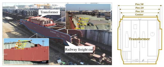
Figure 1.
Railway freight car loaded with a transformer.
Automatic out-of-gauge detection is urgently required to replace manual detection. The existing detection methods can be divided into laser [6], structured light [7], and image-based detection methods [8]. These detection studies provide technical guarantees for railway safety monitoring.
The laser scanner is a representative three-dimensional (3D) data acquisition device that can quickly and accurately reconstruct the three-dimensional entity of the measured item. This method realizes detection by collecting point cloud data, processing point cloud, and three-dimensional reconstruction. Zhang [9] suggested a three-dimensional laser scanning method for the volume of a railway tank car (container). The laser transmitter was installed within the tank car, and the laser receiver received the reflected laser through the tank wall to achieve all-around laser scanning. This method can realize the accurate reconstruction of the railway tank car model, but it is not suitable for measuring the external dimensions of freight trains. Si et al. [10] proposed the application of a laser scanner in large-scale aircraft measurements. However, the aircraft surface is relatively smooth, lacking apparent features and dense point clouds, making detection difficult. Bienert et al. [11] proposed a method to extract and measure individual trees using laser scanning technology automatically. Duan et al. [12] proposed a method to reconstruct shield tunnel lining using point clouds. Shatnawi et al. [13] realized the detection of road ruts using laser scanning. The laser scanner has achieved good performance in an austere environment. However, in complex environments, most dimensional measurement methods for extracting structural key points from 3D point clouds are based on the geometric features of points, with low accuracy. Therefore, the accuracy of the point cloud registration algorithm affects the accuracy of measurement results [14]. At the same time, the particularity of the shape and structure of the measured equipment poses a higher challenge to point cloud registration technology.
The structured light measurement system is widely applicable to various fields of industrial measurement. Wang et al. [15] proposed rail profile recognition based on structured light measurement with depth learning and template matching. The advantages of structured light 3D shape measurement are high precision and high resolution, but the measurable size is limited [16]. In order to solve this scale limitation, Xiao et al. [17] suggested a large-scale structured light 3D shape measurement method combined with reverse photography. In order to improve the accuracy of structured light detection, Xing et al. [18] developed a weighted fusion method based on multiple systems. The structured light measurement system achieves high accuracy under indoor close-distance measurement conditions. However, it is vulnerable to intense natural light outdoors, and the remote measurement accuracy is poor, so it is not suitable for the measurement of railway out-of-gauge freight cars.
With the continuous development of computer vision in recent years, relying on image processing has also become a hot spot for research. Liu [19] presented an algorithm for automatically segmenting railway freight car images. Xie et al. [20] used a stereo-vision measurement technique to achieve freight train gauge-exceeding detection. Chen [21] extracted the train image by processing the video with the three-frame difference method and the Canny operator and finally extracted the vehicle contour information by the minimum rectangle method. Similarly, Han et al. [22] developed a Canny-based edge-detection algorithm to extract and measure the end contours of railway freight cars. Yi et al. [23] proposed an augmented reality-based dynamic detection method to determine if a freight car can pass a particular route by constructing a freight car envelope model and calculating the distance between the freight car envelope and the obstacle. Current image-based research can be roughly divided into edge feature extraction for single images and 3D point cloud reconstruction from multiple image sequences. The measurement range of the first measurement method depends on the installation location and number of cameras, and the accuracy must be improved. In contrast, the second measurement method is too time-consuming, which hinders its promotion to a certain extent. Therefore, current methods struggle to meet the requirements for on-site measurement. Stereo vision is an excellent method for obtaining 3D geometric information about objects. Kim et al. [24] designed a new scheme of crop height measurement methods for agricultural robots based on stereo vision. The measuring range of the binocular measuring system is proportional to the baseline (the distance between two cameras), so the baseline limits the measuring range of the binocular system. In [25], Zhang et al. measured railway freight cars using a large base distance stereo system. To measure huge objects, large-scale measuring equipment should be utilized. Wang [26] developed a mobile stereo-vision system with variable baseline distance to support three-dimensional coordinate measurement in a large field of view.
The standard stereo vision Inspection system’s fixed and short baseline will limit the measurement range and render it ineffective for monitoring large equipment. However, the existing stereo system increases the base distance by adding a fixed guide rail, which will lead to a huge system and cannot meet the requirements of convenience in outdoor industrial applications. Therefore, it is still necessary to explore a flexible stereo vision system with large baseline distance to detect out-of-gauge freight.
Based on the analysis above, we propose a novel measurement system that can change baseline distance with the flight path change through a UAV carrying a single camera. The innovations and contributions of this paper are as follows:
- (1)
- A robust SURF_rBRIEF algorithm for stereo matching is proposed. After testing, the new algorithm’s stability, running speed, and accuracy are improved under different imaging conditions.
- (2)
- Combining with the time-of-flight (TOF) method, the flying altitude control strategy is put forward for measurement with high precision and efficiency.
The rest of this paper is organized as follows. The framework of the visual measurement system is described in Section 2. In Section 3, an analysis of accuracy and control strategy for UAV fixed altitude flight is constructed. As a result, the field verification test is conducted in Section 4. Finally, the conclusions and future work are detailed in Section 5.
2. Visual Measurement Modeling
2.1. Model Description
A mobile single-camera stereo system is a visual measurement technique in which a single camera is moved to capture two frames from different locations against the same target. The system’s cost can be reduced by using only one camera. The camera is moved to various positions, rapidly forming a stereo vision system with varying baseline distances, providing high adaptability. The UAV altitude-holding control method with real-time altitude change compensation is realized by carrying a laser sensor, which further constitutes a mobile single-camera stereo system. An essential aspect of altitude control, hovering the UAV at a specific altitude allows it to acquire stable images from various altitudes.
As depicted in Figure 2, when the UAV is at two different positions, two images containing the same feature point of the heavy-duty railway freight car are captured. The UAV can only ascend or descend in the x (vertical) direction during the flight without any translation or rotation in the z and y (horizontal) directions. This mobile single-camera stereo system overcomes the limitation of the fixed dual-camera stereo system’s baseline spacing. It is possible to construct stereo vision systems with variable baseline spacing by simply moving the camera-equipped UAV to different image acquisition points.
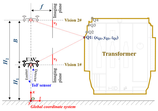
Figure 2.
Single-camera stereo vision system’s measurement principle.
In this paper, the current flight altitude of the UAV is recorded by the time difference between the light generated by the time-of-flight (TOF) sensor bouncing off the ground and returning to the sensor. The UAV takes off vertically in the x-direction from the ground, and if the feature point Q1 is observed for the first time, the height of the UAV from the ground at this position is H1. The coordinates of the image corresponding to the feature point Q1 are p1 = (v1, u1). Next, the UAV moves vertically until the feature point Q1 is no longer visible. When the feature point Q1 is just about to vanish, the UAV’s altitude above the ground is H2. The coordinates of the image corresponding to the feature point Q1 are p2 = (v2, u2). Finally, the mobile stereo system completes the image acquisition, with a baseline B of |H2 — H1| for the system.
The origin of the world coordinate system is located at the projection of the UAV height H1 on the ground, as in Figure 2. The world coordinates of height H1 are supposed as (x1, y1, z1), the world coordinates of height H2 are (x2, y2, z2), and the world coordinates of feature point Q1 are noted as p(xQ1, yQ1, zQ1).
As a result, the world coordinates of H1 can be expressed as (x1, 0, 0) and the world coordinates of H2 can be expressed as (x2, 0, 0). From the geometric relationship, we can obtain
where f is the focal length, (v(1)Q1,u(1)Q1) is the value of the image coordinate system of the point Q1, and the subscript (1) indicates that the position is at height H1. (v(2)Q1,u(2)Q1) is the value of the image coordinate system of the point Q1 and the subscript (2) indicates that the position is at height H2, as in Figure 3.
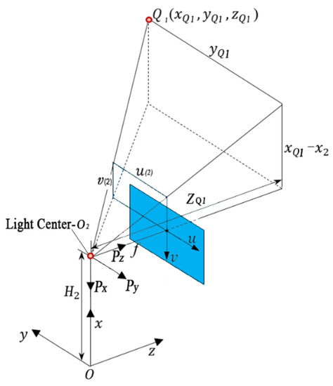
Figure 3.
World coordinates and image coordinates converting relationship.
According to Equation (1), the actual coordinates of the monitoring point can be converted from the image coordinates.
The Di (Disparity) is defined as the difference between the image coordinates captured by the camera carried by the UAV [27]: Di = v(2)Q − v(1)Q. The baseline is: B = x2 − x1 = (v(1)Q − v(2)Q)zQ/f = −Di∙zQ/f. Among them, (xQ, yQ, zQ) represents the point Q coordinates in world coordinate system. Combining Equation (1), we can obtain
As a result, the three-dimensional coordinates of any point can be determined using the image coordinates obtained by the camera at two different positions after conversion. After this point-to-point operation, all points on the image plane can get the corresponding three-dimensional coordinate point cloud as long as there is a corresponding matching point.
2.2. Precision Calculation
As shown in Figure 4, an error analysis model is developed [28]. It is possible to analyze the effects of the baseline and depth of the stereo vision system on measurement precision. Two cameras are placed horizontally to simplify the analysis. The coordinate origin of the vision system is the projection center o1 of the left camera. O1o2 is the stereo vision system baseline with its length equal to B. The effective focal lengths of the two cameras are f1 and f2. The coordinate systems O1u1v1 and O2u2v2 are the image plane coordinate systems corresponding to the left camera and the right camera, respectively. The projection points of the point Q in space on the two image coordinate systems are q1 and q2. The angles between optical axis O1o1, O2o2 and axis x are α1, α2, respectively. The angles between optical axis O1o1, O2o2 and lines Qq1, Qq2 are the projection angles of the field of view of the camera, noted as ω1, ω2, respectively.
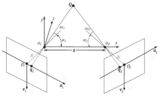
Figure 4.
Model for error analysis.
The three-dimensional coordinates of Q are obtained from the geometric relationship as
Based on Equation (3), the partial derivatives are found for the corresponding functional relations of u1 and u2:
The point Q is assumed to be located at the intersection of the two optical axes of the camera. Two cameras are assumed to be placed symmetrically.
Let , , .
Let ,,,.
The parameter k is introduced to quantify the measurement error e as a function of baseline B. According to the Taylor expansion, we can obtain
The y-direction measuring error at point Q is
The x-direction measuring error at point Q is
Therefore the overall measuring error of the Q point is
As shown in Figure 5, the variation between the baseline, distance, and measurement precision can be derived from the above equation. According to Figure 5a, e2 is closely related to the y-direction measurement accuracy, whereas e1 increases as k increases. Both e2 and e3 exhibit a descending and then ascending trend. The minimum value of e2 is 1, and the corresponding k is 2. The minimum value of e3 is 1.299, and the corresponding k is 1.41. Therefore, if the design of k is between 1 and 2, the system’s accuracy is considered to be high. If k is less than 0.5 or greater than 3, the measurement system is deemed unreliable. According to Figure 5b, once the system’s structure parameter k has been determined, the measurement precision decreases proportionally to the system’s measurement distance.
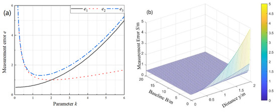
Figure 5.
Measurement precision analysis (a) The effect of k on e (b) The effect of B and y on S.
Taking the DK36 well-hole car loaded with a transformer as an example, we analyzed the requirements of the recognition precision of the freight car contour dimensions on the resolution of the UAV camera. The dimensions of the car are 4.925 × 3.960 (m) and a camera with a × b (pixel) is used for detection. The required detection accuracy is 2 mm. Accuracy is the product of resolution and effective pixels. In general, the effective pixel is 1 in the case of frontal illumination. The camera resolution is 4925/a mm/pixel, so at least 2462.5 pixels are required; therefore, a camera with a resolution of at least 4032 × 3024 (pixel) is used.
2.3. Measurement Scheme
The proposed method consists of four stages: image acquisition and camera calibration, stereo matching, freight car segmentation, and out-of-gauge detection. The calibration of camera parameters is the primary work of vision measurement. The precision of vision measurement results is directly influenced by the precision of calibration results and the stability of the algorithm. Therefore, accurate camera calibration is a prerequisite for effective follow-up work. As the matching ratio of the freight car directly affects the subsequent accuracy of the measurement, stereo matching is the most critical stage. Therefore, an improved image feature extraction and matching methodology, and dynamic threshold are proposed to improve the matching ratio. The freight car segmentation stage aims to extract the freight car and reconstruct the dimension of the freight car. The standard limit graph is constructed by combining the railroad freight train out-of-gauge detection criteria. In the final stage, the out-of-gauge detection is judged by substituting the measurement results into the standard limit graph. More details are provided below.
2.3.1. Image Distortion Correction
In the image-acquisition process, the UAV remains hovering at a fixed flight altitude and ensures that the camera can capture a clear image of the target area at this time. First, when the acquired image contains feature point Q1, the image will be marked as IL. Next, the UAV maintains a smooth and uniform linear flight in the air along the altitude direction from the current observation point position to the following observation point position. When the acquired image no longer contains the feature point Q1, the previous frame of this image will be marked as IR. The baseline distance B is obtained from the difference of the observation point positions corresponding to these two frames. Then, according to the parallax principle, the visual measurement of feature point Q1 is concluded. Last, the steps above are repeated until the final stereo-vision measurements of all feature points have been made. The process is shown in Figure 6, where i is the sequence of image frames, and j is the feature point number.
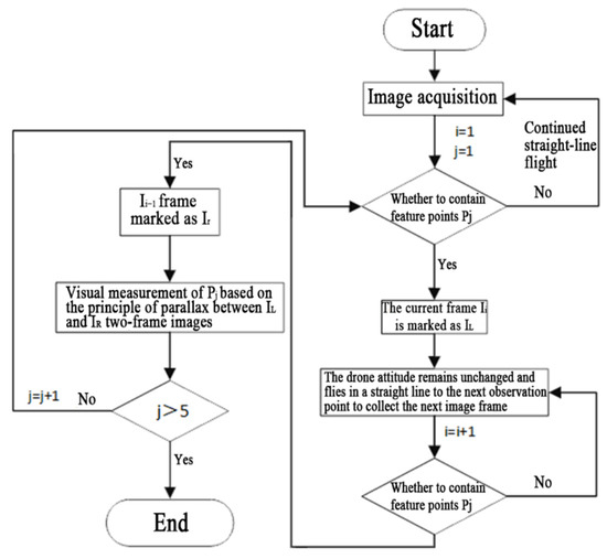
Figure 6.
Image acquisition process.
The LM (Levenberg–Marquardt) algorithm [29] and the gradient descent method [30] were used to solve and analyze the camera models containing different internal parameters, respectively. To determine the internal reference matrix and distortion coefficients, we analyzed the effects of the two algorithms on the calibration accuracy of the camera models to calculate and compare the reprojection errors of the camera models. According to the engineering experience of camera calibration experiments, it is not the case that the more images that are available, the more accurate the calibration results are. The ideal calibration images are between 10 and 20 [31,32], so 15 images are chosen for calibration. The image resolution sizes of the cameras used in the experiments are 4032 × 3024, 5472 × 3648, and 5120 × 3840. The detailed calibration process is given in Figure 7, Figure 8 and Figure 9, which is obtained using a 5 × 7 checkerboard grid image with a grid size of 20 mm × 30 mm and calibrated by the MATLAB Camera Calibration Toolbox [33].
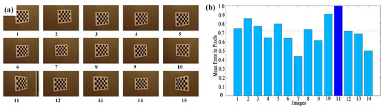
Figure 7.
Camera 1 (Resolution: 4032 × 3024) Calibration process and reprojection error (a) Original image (b) Image reprojection error.
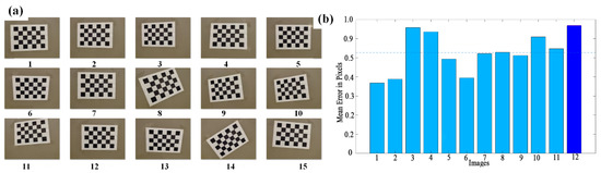
Figure 8.
Camera 2 (Resolution: 5120 × 3840) Calibration process and reprojection error (a) Original image (b) Image reprojection error.
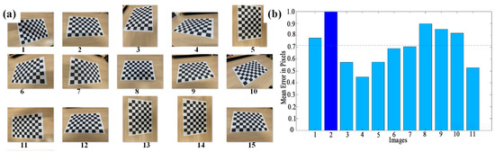
Figure 9.
Camera 3 (Resolution: 5472 × 3078) Calibration process and reprojection error (a) Original image (b) Image reprojection error.
The results of the camera model calibration are shown in Table 1. For the three cameras, compared with the gradient descent method, the reprojection error of the camera calibration model is smaller when optimized using the LM algorithm, and the calibration results of the camera parameters are closer to the ideal values, with an accuracy improvement of 37%. Therefore, the LM algorithm is chosen for the iterative solution of the intra-camera parameters.

Table 1.
Camera model calibration results with different iterative algorithms.
Using the internal parameter matrix and aberration coefficients obtained by solving the calibration experiment, aberration correction can be applied to the images captured by the camera. After aberration correction, the images captured by cameras with different aberration coefficients exhibit distinct effects. Figure 10 shows the comparison before and after the correction of the freight car images captured by UAV, where Figure 10a shows the original image of the DK36 well-hole car captured by UAV, and Figure 10b shows the correction result. Compared with the image taken by the UAV before correction, the lines at the edge of the freight car and the rails at the front of the image are restored from the curve shown in Figure 10a to a straight state, as shown in Figure 10b, and the correction effect is more pronounced. Therefore, for the camera lens with more serious distortion, it must be processed by the imaging distortion correction model to obtain the accurate image pixel coordinates.
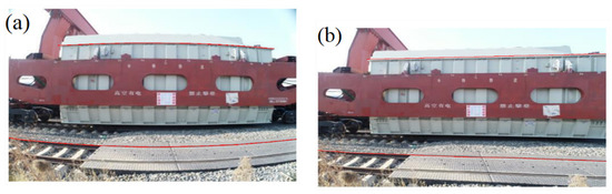
Figure 10.
Image distortion correction effect (a) Raw image captured by UAV (b) Corrected image.
2.3.2. Image Feature Matching
For image feature matching, the SURF_rBRIEF algorithm is presented in this paper. The SURF_rBRIEF algorithm is created by combining the SURF detector [34] and the rBRIEF descriptor [35]. The matching point screening process can dynamically adapt to different matching algorithms due to the improved coarse matching threshold. The SURF detector can obtain many stable feature points with better robustness in the feature point-detection phase. The rBRIEF descriptor is fast in computation, occupies little memory, has rotational invariance, and is more accurate in grasping the information of feature points. Therefore, an improved algorithm coupled with these two algorithms, SURF_rBRIEF, is proposed in this paper. The basic idea of this algorithm is described herein. First, the SURF_rBRIEF algorithm is the same as SURF in the feature point-detection stage. The SURF algorithm is used to obtain feature point localization. Next, the main direction of the point is obtained according to the grayscale center-of-mass method. Then, the descriptors are calculated by the rBRIEF method. Finally, the key points and descriptors of the feature points are obtained. The flow of the SURF_rBRIEF feature point detection and matching algorithm is shown in Figure 11.
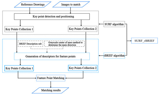
Figure 11.
Process of SURF_rBRIEF’s feature point detection and matching.
For accurate matching, a new coarse matching threshold is proposed. The screening threshold ε for coarse matching and the interval [Dmin, Dmax] of the matching distance D are dynamically linked. When the detection algorithm is modified, the coarse matching threshold will be dynamically adjusted based on the matching distance interval to filter out incorrect matches, which may guarantee a sufficient number of matching point pairs and improve matching results. The dynamic threshold can be expressed as
In order to compare the original SURF algorithm with the improved SURF_rBRIEF, the performance of the algorithm under different imaging conditions was tested. There were five types of variations in the imaging conditions during image acquisition: point-of-view variation, scale variation, blurring, JPEG compression, and illumination conditions. The experimental environment was Ubutun18.04, Linux operating system, Intel Core i5-9300H CPU @2.40GHz, and OpenCV3.4.4. The coarse matching strategy was used for both algorithms in the test, and the coarse matching threshold was changed dynamically according to the description of the sub-distance interval. The matching was carried out uniformly utilizing the Hamming distance matching method [36]. The experimental dataset was derived from Mikolajczyk’s [37] publicly accessible image database. The algorithm’s test data results in a successful state are summarized in Table 2 below. In conclusion, the proposed SURF_rBRIEF algorithm improved the stability, running speed, and accuracy under different imaging conditions compared to the original SURF algorithm. The overall accuracy increased by 21%, and the running speed increased by 52%.
Table 2.
Comparison of experimental results of SURF and SURF_rBRIEF algorithms.
Actual measured image data of DK36 well-hole cars were used to verify that the algorithm can achieve stable feature extraction and match in critical parts of railway freight cars. During the UAV flight, images of various railway freight car parts were collected and processed using the SURF and SURF_rBRIEF algorithms for comparison and analysis. Figure 12a,c show the image feature extraction and matching effect obtained by using the SURF algorithm at different parts of the body of the DK36 well-hole car, respectively. Figure 12b,d show the image feature extraction and matching effect obtained by using the improved SURF_rBRIEF algorithm at different parts of the body of the DK36 well-hole car, respectively. Comparing the matching effects in Figure 12, we can see that for the images of the top and bottom body parts of the DK36 well-hole car collected by the UAV, the newly proposed SURF_rBRIEF algorithm in this paper has fewer error matching line segments, indicating that the improved algorithm has fewer error matching points and higher accuracy compared with the original SURF algorithm.
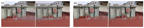
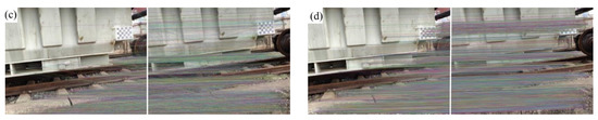
Figure 12.
Image feature matching results of DK36 well-hole car (a) SURF algorithm at top (b) SURF_rBRIEF algorithm at top (c) SURF algorithm at bottom (d) SURF_rBRIEF algorithm at bottom.
2.3.3. Image Target Segmentation
The image segmentation technique was used to rapidly locate critical parts of heavy-duty railway freight cars and disassemble them. It was followed by rapid reconstruction of freight train contours and out-of-gauge detection combined with stereo matching. Since the HSV color space is closer to human visual perception of color, the RGB color space is first converted to HSV color space. The freight train is initially segmented based on color [38] to obtain the freight train outline information with the background removed. Then, the edge features of the freight train were obtained by the Canny operator [39], and a total of P horizontal linear edge points were extracted and fitted to the straight line using the RANSAC (random sample consensus) method [40]. We set the edge point set as P, and the key steps of the algorithm for determining the straight line of the car’s edge profile are as follows. First, the line equation is written as ax + by = 1, where a and b are the equation coefficients that two points can solve. Next, two randomly selected points, Pi and Pj, are used to calculate coefficients a and b. Then, the distances from all other points to the line obtained from a and b are computed. Moreover, the number of points whose distance is smaller than threshold dt is counted and forms an inlier point set S. Furthermore, the above steps are repeated M times and the fitted line with the highest number of internal points Smax is selected. Finally, the coefficients of the corresponding lines are recorded as a′ and b′. Figure 13 shows the segmentation process of the image of a heavy-duty railway freight train.
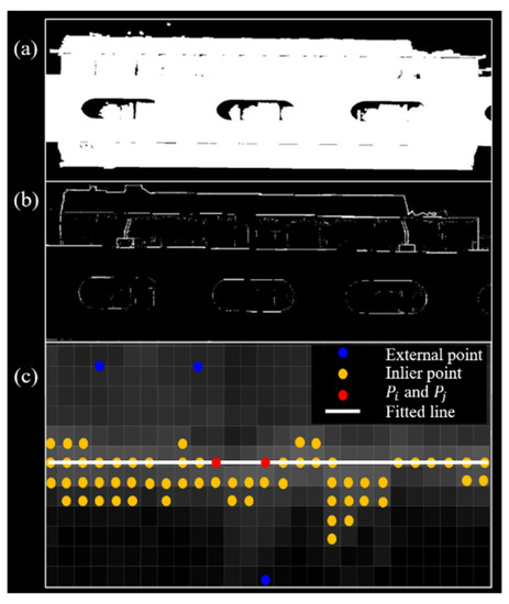
Figure 13.
Rapid freight train segmentation (a) Localization (b) Edge point extraction (c) Straight line fitting.
3. Flying Altitude Control Strategy
3.1. Controlling Precision Analysis
Since there is an accuracy error in the altitude holding control of the UAV during the fixed altitude flight, it is necessary to analyze the impact of the flight altitude positioning error on the measurement accuracy. The UAV is assumed to ascend at an altitude of B (the baseline distance of the optical center) and the altitude holding accuracy error is ∆B. As a result, the image position of the feature point at the first position remains unchanged as (u(1)Q, v(1)Q), while the image coordinates of the feature point at the second position become (u(2)Q, v(2)Q). From Equation (1), we obtain
where is the z-axis coordinate in the world coordinate value of the observation point. When the actual translation distance (B + ΔB) of the camera’s optical center baseline, the actual imaging coordinates are as follows:
where (xQ, yQ, zQ) is the world coordinate of the observation point, (u′(1)Q, v′(1)Q) is the actual image coordinate of the observation point, and (x1, y1, z1) is the world coordinate of the camera.
Substituting Equation (13) into Equation (12), the baseline remains B because the actual spatial coordinates do not change. In conjunction with Equation (2), (x′Q, y′Q, z′Q) can be derived by the following:
Let ΔxQ = x′Q − xQ, ΔyQ = y′Q − yQ, and ΔzQ = z′Q − zQ. Combining Equation (14), the generalized equation for UAVs’ altitude holding altitude accuracy control can be written as follows:
According to Equation (15), when the object distance is zQ and the UAV carrying the camera with focal length f and baseline B, in order to reduce the distance error ΔzQ, it can be achieved by increasing the baseline B. When the baseline is 2.5 m, the UAV positioning error ∆B is 1 mm, and the object distance zQ is 3 m, the measurement error ΔzQ can be controlled to 1.2 mm.
As a result, the baseline B and the distance between the UAV and the photographed object can thus be adjusted according to the UAV equipment’s positioning accuracy and measurement requirements. The above equations hold, ensuring that the reconstruction model’s precision meets the measurement specifications.
3.2. Altitude Holding Strategy
At this stage, the UAV altitude holding accuracy is greatly affected by the equipment hardware conditions and environmental factors, which lead to being not stable enough in the flight control process. DJI PHANTOM 4 RTK was used as the UAV, with the hovering accuracy shown in Table 3.
Table 3.
Hovering accuracy of the UAV PHANTOM 4 RTK (unit: m).
Table 3 shows that the hovering accuracy of the current UAV is generally controlled within the meter-level error. It will lead to the measurement error value being further amplified by the presence of UAV hovering error in the stereo 3D reconstruction theoretical model of UAV fixed altitude control. Increasing the baseline is an option to compensate for this error value. However, in the practical application of stereo vision, when the baseline is too large, and the camera is too close to the object, it is difficult for the camera to capture images in the same area at two different positions. These images can easily result in the failure of subsequent image feature matching, thereby causing the failure of visual measurement. Therefore, this paper proposes a laser sensor-equipped altitude control method. The altitude holding control method of UAV with laser sensor is mainly by actively transmitting laser pulses to the ground and sensing the distance change based on the reflected signals. The time-of-flight (TOF) method [41] has a high degree of measurement precision. The measurement error is relatively stable within the range, so it is selected to obtain the UAV flight altitude information, then used as altitude control following processing by the flight controller’s altitude loop.
As shown in Figure 14a, the laser range was measured by the TF-Solar07 sensor, which had a measuring range of 12 m and an accuracy of 1 mm. After the sensor acquired altitude data, it was first processed by the Kalman filter [42] before being processed by the altitude channel and then used to control the UAV’s altitude. The filtered results are shown in Figure 14b. The measurement results were filtered to reduce measurement errors due to fluctuations, resulting in smoother data. Consequently, UAV’s altitude is controlled within the centimeter-level error.
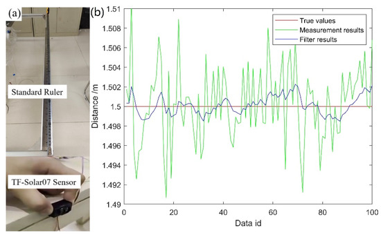
Figure 14.
Measurement processes (a) Measurement equipment (b) Measurement and filtering results.
To enhance the system’s anti-interference capabilities and make the UAV more altitude-adaptive, the altitude/speed cascade proportional–integral–derivative (PID) control algorithm [43] was used for altitude control, whose principle is depicted in Figure 15. The inner loop of the tandem PID is the speed closed loop, and the outer loop is the altitude closed loop.
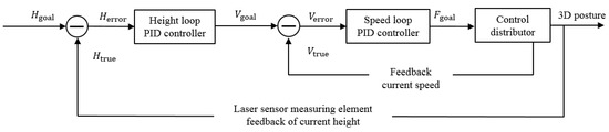
Figure 15.
Altitude control method.
A proportional–integral (PI) controller is used to control the altitude closed loop, whose output value is the desired speed. The proportional term adjustment can quickly compensate for disturbances, while the integral term adjustment can eliminate residuals.
where is the scaling factor of the outer ring and is the integration factor of the outer ring.
A proportional–integral–derivative (PID) controller is used for closed-loop control of the speed. Its output is the desired pull, where the differential term adjustment increases the system’s stability.
where m is the total mass of the UAV, g is the acceleration of gravity, is the scale factor of the inner ring, is the integration factor of the inner ring, and is the differentiation factor of the inner ring.
4. Validation and Application
A field test was conducted at a yard in Shenyang, Liaoning Province, China, with a DK36 well-hole car loaded with a transformer. Based on the model framework and algorithm flow established in the previous paper, a measurement scheme for the loading contour dimensions of out-of-gauge freight cars was developed, and the contour dimensions of the DK36 well-hole car were measured and calculated. Eventually, the calculated results were compared with the actual measurement results to prove the validity of the model and to analyze the factors affecting the model error. In order to verify the accuracy and efficiency of our measurement system, we used manual and UAV measurements to detect the out-of-gauge freight car, as shown in Figure 16.
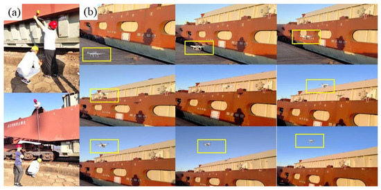
Figure 16.
Comparison of measurement process between manual method and UAV method (a) Manual measurement (b) UAV flight measurement.
For the well-hole car loaded with a transformer, the measurement staff is not concerned with the length of the train but rather with the width and height of four special positions. These four unique positions are the center, pos 1#, pos 2#, and pos 3#. The center position refers to the transformer’s uppermost position, the second side position refers to the lugs on both sides of the transformer, and the third side position refers to the vehicle’s side-bearing beams on both sides. Figure 17 shows the distribution of the points and locations to be measured. Number 1 and 2 are used to determine the height of the center position. Number 3 and 4 are used to determine the height of the Pos 1#. Number 5 and 6 are used to determine the height of the Pos 2#. Number 7 and 8 are used to determine the height of the Pos 3#. Number 9 and 10 are used to determine the width of the center position. Number 11 and 12 are used to determine the width of the Pos 1#. Number 13 and 14 are used to determine the width of the Pos 2#. Number 15 and 16 are used to determine the width of the Pos 3#. The focal length of the camera used in the experiment is 35 mm. The baseline B is 2 m. The UAV shooting heights H1 and H2 are 1.5 m and 3.5 m, respectively. The object distance ZQ is between 4.5 and 4.7 m depending on the observation point. As shown in Figure 18, the images taken by UAV were matched for stereo recognition.
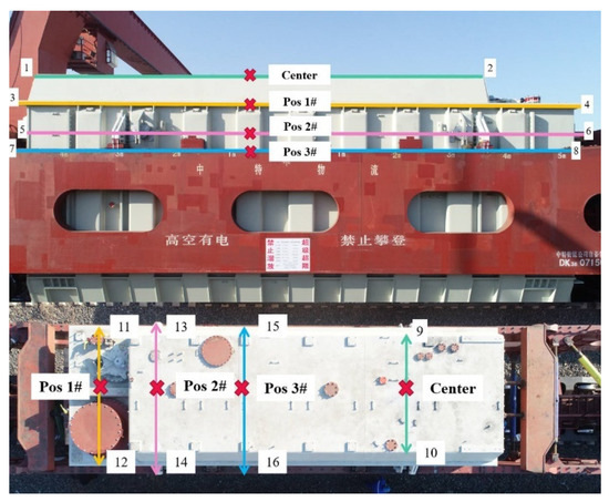
Figure 17.
Measuring parts of the DK36 well-hole car.
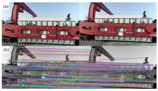
Figure 18.
Stereo recognition process (a) Stereo images (b) Image matching results.
The contour dimensions of the DK36 well-hole car were measured by both UAV stereo recognition and manual measurement. The captured images were extracted with feature points and reconstructed with the help of the SURF_rBRIEF algorithm, and the contour dimensions were finally calculated. Table 4 and Table 5 show the coordinates of observation points and contour width dimensions obtained by the two measurement methods.
Table 4.
Measurement results of points.
Table 5.
Measurement results of DK36 well-hole car.
The manual measurement took two hours, while the UAV detection method proposed in this paper only took five minutes. According to the experimental results in Table 5, compared with manual measurement, the width and height measurement relative error of the DK36 well-hole car measured by UAV is within 3.80%, with an average error of 3.29%. Because there is no complex point cloud reconstruction, we could carry out rapid two-dimensional detection but could not obtain an accurate three-dimensional model of the DK36 well-hole car. The position with the smallest relative error is the center width. The standard boundary graph was constructed according to the railroad freight train out-of-gauge detection standard. The measurement results were compared with the fundamental building limits in the railroad limit contour, and the results were obtained, as shown in Figure 19. The top-loading dimension of this DK36 well-hole car was within the primary building limit, but some positions slightly exceeded the maximum overload cargo loading limit.
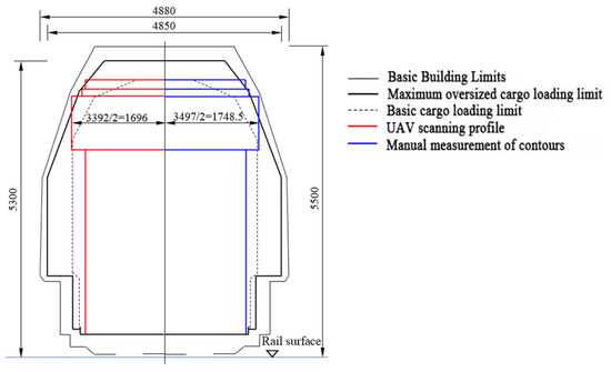
Figure 19.
Out-of-gauge detection result.
5. Conclusions
In this paper, a freight train out-of-gauge stereo vision-detection method based on a radar-assisted and single-camera-equipped UAV was presented. The 2D model of the train was reconstructed from stereo images and then compared with the railway gauge according to national standards, thus completing the out-of-gauge detection much faster than the 3D model. The SURF_rBRIEF algorithm was used to ensure the measuring accuracy, and the time-of-flight (TOF) method was used to hold altitude for robustness. The principle of the vision measurement system was described and the factors which affect measuring accuracy were analyzed. The image matching experiments confirm the better adaptability of our method to complex practical applications. The on-site experiment shows that the railway freight car measurement error is less than 0.18 m and the relative error is within 3.8%. All experiments prove the robustness, high precision, and efficiency of the method.
Although our image-matching algorithm was tested by the lighting data set, the test system was not verified under extreme lighting conditions such as night. The measurement system will also be disabled if the UAV flight is restricted by extreme weather, such as rain and snow. In future work, the identification of different types of railway freight cars and optimization during extreme severe weather are needed to achieve better performance.
Author Contributions
J.L.: data curation, writing original draft, software, visualization; W.Z.: conceptualization, methodology, project administration, supervision, investigation, writing—review and editing. W.G. and Z.L.: resources, writing—review and editing, investigation, project administration; H.Y. and W.W.: resources, writing—review and editing, investigation, project administration; Z.W., C.S. and J.P.: resources, writing—review and editing, investigation, project administration. All authors have read and agreed to the published version of the manuscript.
Funding
This research was supported by the Special Heavy Load Topic of Science and Technology Research and Development Plan of China Railway Taiyuan Bureau Group Co., Ltd. (Grant no. A2021J04), the Fundamental Research Funds for the Central Universities of Central South University (Grant no. 2022ZZTS0754), the Postgraduate Scientific Research Innovation Project of Hunan Province (Grant no. 2021XQLH021), and the National Key R&D Program of China (Grant no. 2016YFB1200402).
Data Availability Statement
Not applicable.
Acknowledgments
We would like to acknowledge the reviewers and editors for their valuable comments and suggestions.
Conflicts of Interest
The authors declare no conflict of interest.
References
- Petraska, A.; Jarasuniene, A.; Ciziuniene, K. Routing Methodology for Heavy-Weight and Oversized Loads Carried by Rail Transport. Procedia Eng. 2017, 178, 589–596. [Google Scholar] [CrossRef]
- Xiang, H.; Mou, R.F. Optimization of Loading Scheme on Railway Dangerous Goods|ICTE 2019. Available online: https://ascelibrary.org/doi/abs/10.1061/9780784482742.053 (accessed on 7 November 2022).
- Jin, X.; Xiao, X.; Ling, L.; Zhou, L.; Xiong, J. Study on Safety Boundary for High-Speed Train Running in Severe Environments. Int. J. Rail Transp. 2013, 1, 87–108. [Google Scholar] [CrossRef]
- Khajehei, H.; Ahmadi, A.; Soleimanmeigouni, I.; Haddadzade, M.; Nissen, A.; Latifi Jebelli, M.J. Prediction of Track Geometry Degradation Using Artificial Neural Network: A Case Study. Int. J. Rail Transp. 2022, 10, 24–43. [Google Scholar] [CrossRef]
- Bernal, E.; Spiryagin, M.; Cole, C. Onboard Condition Monitoring Sensors, Systems and Techniques for Freight Railway Vehicles: A Review. IEEE Sens. J. 2018, 19, 4–24. [Google Scholar] [CrossRef]
- Zhao, W.C.; Xu, X.Z.; Le, Y. System design and implementation for a portable laser rangefinder with dual detectors. J. Cent. South Univ. (Sci. Technol.) 2015, 46, 7. (In Chinese) [Google Scholar]
- Zhang, G.Y.; Ding, X.D.; Lu, G.Y. Railway out-of-gauge detection system establishment and experiment research based on combination of infrared and high-speed video camera technology. China Transp. Rev. 2017, 39, 6. (In Chinese) [Google Scholar]
- Sun, L.L.; Xiao, S.D. Algorithm research on freight train gauge inspection system based on structure lighting theorem. Comput. Appl. 2005, 25, 3. (In Chinese) [Google Scholar]
- Zhang, Z. A New Measurement Method of Three-Dimensional Laser Scanning for the Volume of Railway Tank Car (Container). Measurement 2021, 170, 108454. [Google Scholar] [CrossRef]
- Si, H.; Qiu, J.; Li, Y. A Review of Point Cloud Registration Algorithms for Laser Scanners: Applications in Large-Scale Aircraft Measurement. Appl. Sci. 2022, 12, 10247. [Google Scholar] [CrossRef]
- Bienert, A.; Georgi, L.; Kunz, M.; von Oheimb, G.; Maas, H.-G. Automatic Extraction and Measurement of Individual Trees from Mobile Laser Scanning Point Clouds of Forests. Ann. Bot. 2021, 128, 787–804. [Google Scholar] [CrossRef]
- Duan, D.Y.; Qiu, W.G.; Cheng, Y.J.; Zheng, Y.C.; Lu, F. Reconstruction of Shield Tunnel Lining Using Point Cloud. Autom. Constr. 2021, 130, 103860. [Google Scholar] [CrossRef]
- Shatnawi, N.; Obaidat, M.T.; Al-Mistarehi, B. Road Pavement Rut Detection Using Mobile and Static Terrestrial Laser Scanning. Appl. Geomat. 2021, 13, 901–911. [Google Scholar] [CrossRef]
- Gojcic, Z.; Zhou, C.; Wegner, J.D.; Guibas, L.J.; Birdal, T. Learning Multiview 3d Point Cloud Registration. In Proceedings of the IEEE/CVF Conference on Computer Vision and Pattern Recognition, Seattle, WA, USA, 14–19 June 2020; pp. 1759–1769. [Google Scholar]
- Wang, S.; Wang, H.; Zhou, Y.; Liu, J.; Dai, P.; Du, X.; Abdel Wahab, M. Automatic Laser Profile Recognition and Fast Tracking for Structured Light Measurement Using Deep Learning and Template Matching. Measurement 2021, 169, 108362. [Google Scholar] [CrossRef]
- Vargas, R.; Romero, L.A.; Zhang, S.; Marrugo, A.G. Toward High Accuracy Measurements in Structured Light Systems. In Proceedings of the Dimensional Optical Metrology and Inspection for Practical Applications XI, Orlando, FL, USA, 31 May 2022; Volume 12098. [Google Scholar] [CrossRef]
- Xiao, Y.L.; Wen, Y.; Li, S.; Zhang, Q.; Zhong, J. Large-Scale Structured Light 3D Shape Measurement with Reverse Photography. Opt. Lasers Eng. 2020, 130, 106086. [Google Scholar] [CrossRef]
- Xing, C.; Huang, J.; Wang, Z.; Gao, J. A Multi-System Weighted Fusion Method to Improve Measurement Accuracy of Structured Light 3D Profilometry. Meas. Sci. Technol. 2022, 33, 055401. [Google Scholar] [CrossRef]
- Liu, L.; Zhou, F.; He, Y. Automated Status Inspection of Fastening Bolts on Freight Trains Using a Machine Vision Approach. Proc. Inst. Mech. Eng. Part F J. Rail Rapid Transit 2016, 230, 1629–1641. [Google Scholar] [CrossRef]
- Xie, F.; Zhang, X.P.; Zhang, Y.X.; Wang, S.; Xu, J.Z. Exterior Orientation Calibration Method for Freight Train Gauge-Exceeding Detection Based on Computer Vision. J. China Railw. Soc. 2012, 34, 72–78. [Google Scholar]
- Chen, L.Y. Research and Design of Outer Contour Overrun Detection of Vehicle Based on Machine Vision. Master’s Thesis, Changsha University of Science & Technology, Changsha, China, 2015. (In Chinese). [Google Scholar]
- Han, Y.; Qiao, M.; Wan, X.; Chang, Q. Application of Image Analysis Based on Canny Operator Edge Detection Algorithm in Measuring Railway Out-of-Gauge Goods. Adv. Mater. Res. 2014, 912–914, 1172–1176. [Google Scholar] [CrossRef]
- Yi, B.; Sun, R.; Long, L.; Song, Y.; Zhang, Y. From Coarse to Fine: An Augmented Reality-Based Dynamic Inspection Method for Visualized Railway Routing of Freight Cars. Meas. Sci. Technol. 2022, 33, 055013. [Google Scholar] [CrossRef]
- Kim, W.S.; Lee, D.H.; Kim, Y.J.; Kim, T.; Lee, W.-S.; Choi, C.-H. Stereo-Vision-Based Crop Height Estimation for Agricultural Robots. Comput. Electron. Agric. 2021, 181, 105937. [Google Scholar] [CrossRef]
- Zhang, Y.; Wang, S.; Zhang, X.; Xie, F.; Wang, J. Freight Train Gauge-Exceeding Detection Based on Three-Dimensional Stereo Vision Measurement. Mach. Vis. Appl. 2013, 24, 461–475. [Google Scholar] [CrossRef]
- Wang, Y.; Wang, X. A Mobile Stereo Vision System with Variable Baseline Distance for Three-Dimensional Coordinate Measurement in Large FOV. Measurement 2021, 175, 109086. [Google Scholar] [CrossRef]
- Qi, L.; Zhang, X.; Wang, J.; Zhang, Y.; Wang, S.; Zhu, F. Error Analysis and System Implementation for Structured Light Stereo Vision 3D Geometric Detection in Large Scale Condition. SPIE 2012, 8555, 350–357. [Google Scholar]
- Zhang, G.J. Machine Vision; Science Press: Beijing, China, 2005. [Google Scholar]
- Moré, J.J. The Levenberg-Marquardt Algorithm: Implementation and Theory. In Numerical Analysis; Watson, G.A., Ed.; Springer: Berlin/Heidelberg, Germany, 1978; pp. 105–116. [Google Scholar]
- Ruder, S. An Overview of Gradient Descent Optimization Algorithms. arXiv 2016, arXiv:1609.04747 2016. [Google Scholar]
- Zhang, Z.Y. Flexible Camera Calibration by Viewing a Plane from Unknown Orientations. In Proceedings of the Seventh IEEE International Conference on Computer Vision, Kerkyra, Greece, 20 September 1999; Volume 1, pp. 666–673. [Google Scholar]
- Fetić, A.; Jurić, D.; Osmanković, D. The Procedure of a Camera Calibration Using Camera Calibration Toolbox for MATLAB. In Proceedings of the 2012 35th International Convention MIPRO, Opatija, Croatia, 21–25 May 2012; pp. 1752–1757. [Google Scholar]
- Bouguet, J.Y. Camera Calibration Toolbox for Matlab. Available online: http://robots.stanford.edu/cs223b04/JeanYvesCalib/index.html (accessed on 4 December 2003).
- Bay, H.; Tuytelaars, T.; Van Gool, L. SURF: Speeded Up Robust Features. In Computer Vision—ECCV 2006; Leonardis, A., Bischof, H., Pinz, A., Eds.; Springer: Berlin/Heidelberg, Germany, 2006; pp. 404–417. [Google Scholar]
- Huang, W.; Wu, L.-D.; Song, H.-C.; Wei, Y.-M. RBRIEF: A Robust Descriptor Based on Random Binary Comparisons. IET Computer Vision 2013, 7, 29–35. [Google Scholar] [CrossRef]
- Awaludin, M.; Yasin, V. Application Of Oriented Fast And Rotated Brief (Orb) And Bruteforce Hamming In Library Opencv For Classification Of Plants. J. Inf. Syst. Appl. Manag. Account. Res. 2020, 4, 51–59. [Google Scholar]
- Sedaghat, A.; Ebadi, H. A Performance Evaluation of Local Descriptors. Iran. J. Remote Sens. GIS 2016, 7, 61–84. [Google Scholar]
- Sural, S.; Qian, G.; Pramanik, S. Segmentation and Histogram Generation Using the HSV Color Space for Image Retrieval. In Proceedings of the International Conference on Image Processing, Rochester, NY, USA, 22–25 September 2002; Volume 2, p. II. [Google Scholar]
- Medina-Carnicer, R.; Muñoz-Salinas, R.; Yeguas-Bolivar, E.; Diaz-Mas, L. A Novel Method to Look for the Hysteresis Thresholds for the Canny Edge Detector. Pattern Recognit. 2011, 44, 1201–1211. [Google Scholar] [CrossRef]
- Derpanis, K.G. Overview of the RANSAC Algorithm. Image Rochester NY 2010, 4, 2–3. [Google Scholar]
- Schaart, D.R. Physics and Technology of Time-of-Flight PET Detectors. Phys. Med. Biol. 2021, 66, 09TR01. [Google Scholar] [CrossRef]
- Menegaz, H.M.; Ishihara, J.Y.; Borges, G.A.; Vargas, A.N. A Systematization of the Unscented Kalman Filter Theory. IEEE Trans. Autom. Control 2015, 60, 2583–2598. [Google Scholar] [CrossRef]
- Izci, D. Design and Application of an Optimally Tuned PID Controller for DC Motor Speed Regulation via a Novel Hybrid Lévy Flight Distribution and Nelder–Mead Algorithm. Trans. Inst. Meas. Control 2021, 43, 3195–3211. [Google Scholar] [CrossRef]


Publisher’s Note: MDPI stays neutral with regard to jurisdictional claims in published maps and institutional affiliations. |
© 2022 by the authors. Licensee MDPI, Basel, Switzerland. This article is an open access article distributed under the terms and conditions of the Creative Commons Attribution (CC BY) license (https://creativecommons.org/licenses/by/4.0/).