A Control Algorithm for Early Wildfire Detection Using Aerial Sensor Networks: Modeling and Simulation  ^†

Abstract

This work presents an algorithm for an Aerial Sensor Network (ASN) composed of fixed-wing Unmanned Aerial Vehicles (UAVs) that performs surveillance and detects the early signs of a wildfire in a given territory. The main goal is to cover a given area while prioritizing areas of higher fire hazard risk. The proposed algorithm is scalable to any number of aircraft and can use any kind of fire hazard risk map as long as it contains bounded and nonnegative values. Two different dynamical models associated with the movement of fixed-wing UAVs are proposed, tested, and compared through simulations. Lastly, we propose a workflow to size the ASN in order to maximize the probability of detection of wildfires for a particular risk profile.

1. Introduction

1.1. Motivation

During 2017, a burnt area in Portugal saw a 428% increase relative to its mean values, as reported in [1]. In particular, the wildfire of Pedrógão Grande resulted in a burnt area of nearly 45.039 acres [1], causing nearly 500 million euros of estimated damage to the Portuguese government [2]. In fact, Portugal holds the largest percentage of burned area in Europe and is also the country in Europe with the highest number of ignitions per 1000 inhabitants. When compared to Spain, which has a similar climate and vegetation, Portugal has 6 times more fires per 1000 inhabitants [3].

While the cause of the previously mentioned fire was unrelated to human activity, rural fire activity in Portugal is often caused by humans. Between the years of 2011 and 2021, 48% of the fires with known causes were caused by the inappropriate use of controlled fire as reported by Instituto da Conservação da Natureza e das Florestas in [4]. More specifically, 31% are caused by controlled the burns of forest debris and agriculture excess that, by negligence, became out of control. In addition, 23% of fires are caused by criminal activity. This data is further corroborated in [5], which expanded the scope to all fire types instead of just rural and obtained similar proportions.

The consequences of human negligence and human criminal activity are that fires of a small dimension start on the forest surface and spread until they become uncontrollable.

In light of these statistics, it is of extreme importance that an efficient method to cover an area under high risk of ignition and subject to frequent human activity is developed, so that the firefighting personnel are made aware of ignitions before they devolve and become uncontrollable.

1.2. Literature Review

The ideal fire detection solution would be one that maintains continuous coverage of an area and is able to identify all sources of ignition. Geostationary satellites satisfy the first requirement and are already used to monitor environmental phenomena. However, due to the high orbit altitude, approximately 36,000 km, the resolution of the obtained data is very low. One example of this is the Visible Spin Scan Radiometer Atmospheric Sounder (VAS) sensor of the Geostationary Operational Environmental Satellite (GOES) satellite, which produces samples of wildfires every three hours with a resolution between 7 and 14 km on the infrared wavelength [6]. There is the possibility of reducing the satellite’s orbit altitude to increase the spatial resolution, however there is less availability of such services.

A lower altitude example is the data gathered in [1], taken from the moderate resolution imaging spectroradiometer (MODIS) sensor with a resolution of 250 m, but is limited to four overpasses in a 24-h period. In addition, data from such measurements can be corrupted by cloud cover [7].

Ground-based detection systems are much cheaper than satellite solutions and are not susceptible to corruption from cloud cover. These provide continuous coverage using a visible and subvisible optical sensor, but have very low mobility and are limited to line-of-sight measurements, which can be obstructed by terrain features [8].

This work focuses on Aerial Sensor Networks (ASNs) consisting of fixed-wing Unmmaned Aerial Vehicles (UAVs) as a means to cover a given area. Unlike satellite solutions, the deployment of an ASN allows firefighting personnel to focus on a particular area of interest by obtaining high resolution data [9]. In particular, we favor optimal resource allocation in the sense that regions of higher risk should be monitored more often than areas with a lower risk.

Many different measures of risk can be found in [10]. The different measures of risk are mostly based on the economical damage that a wildfire at any given location would cause, weighted by the probability of an ignition in said area. In the case of the Portuguese territory, different measures of risk have been considered in the past, including, for example:

• The approach in [11], which provides a method for the construction of an ignition probability map based on landscape and human-related variables;
• The Canadian Fire Weather Index (FWI), which combines the probability of an ignition with a wildfire propagation model in order to evaluate the risk of a wildfire, as described in [12]. This index is currently used by the Instituto Português do Mar e da Atmosfera (IPMA) in Portugal [13];
• The method in [14], which builds a hazard map from wildfire susceptibility and wildfire probability maps.

Both the approaches in [11,14] have difficulty assessing the risk caused by human presence, something that is detrimental to any ASN using risk maps generated through these approaches, since the majority of fires in Portugal is caused by humans (see [4,5,15]), as previously mentioned.

With the risk function for a given area, a method is required to guide agents in the ASN to places with higher risk values more often. The survey [16] describes a number of different strategies for both single and multi-robot area coverage. This problem is related to the so-called “lawnmower problem”, which consists of the determination of a path that covers a given area and the “watchman’s route problem”, which determines the best route to scan the given area. These problems become increasingly difficult as constraints are added to the system, such as the presence obstacles, Field of View (FOV) restrictions, and dynamical constraints. While UAVs are usually not constrained by the presence of obstacles (if their altitude is high enough), they may be subject to dynamical constraints and the onboard sensors may be subject to FOV restrictions. Some of these problems are addressed in [17] and, notably, the authors in [18] follow an approach where point-mass vehicles are routed to areas of higher priority more often.

As stated before, these coverage algorithms can be used in cooperative control with different constraints and objectives. The work in [9] solves the vehicle routing problem optimally with respect to a cost function that minimizes the time it takes to cover a given area, while taking into account the limitations of the vehicles. In [19,20], a team of quad-copters is coordinated so as to perform the continuous surveillance of a given area while avoiding collisions.

1.3. Objectives

The objective of this work is to develop a real time trajectory generation algorithm that is capable of allocating resources from a ASN of fixed-wing UAVs based on the fire hazard risk map on a certain domain, with the goal of maximizing the probability of detecting an ignition.

In order to achieve this goal, the approach used in [18] was chosen as the starting point. The control law developed in the article does exactly what is necessary: It takes a risk map with very little constraints and guides a network of point-mass agents towards zones with high priority. The dynamical systems used in [18] can not be used directly in a real mission, however, because they do not take into account vehicle dynamics. In this work, the control law is adapted in order to take into consideration the dynamics of fixed-wing UAVs.

1.4. Organization

This work is divided in three Sections. In Section 2, all the concepts and variables needed to obtain the final control law are defined and explained, as well as the definition of the dynamical systems that describe the motion of an UAV. In Section 3, the control laws obtained in Section 2 section will be tested in a MATLab/Simulink environment. In Section 4, a probabilistic model will be developed to take into account sensor capabilities, as well as to define exactly what needs to be detected and how it will be detected.

2. Uniform Coverage with Fixed-Wing Unmanned Aerial Vehicles

In this work, we borrow the metric for uniform coverage from [18] and we present it in the next section for the sake of completeness.

2.1. The Metric for Uniform Coverage

Given a set of N agents for an ASN, let the following distribution $C^t$ be defined:

$$C^t\left(\mathbf{x}\right)=\frac{1}{Nt}{\int }_0^t\sum _{j=1}^N\delta (\mathbf{x}-{\mathbf{x}}_j\left(\tau \right))d\tau ,$$

(1)

for each $\mathbf{x}\in {\mathbb{R}}^n$, where ${\mathbf{x}}_j:[0,t]\to {\mathbb{R}}^n$ represents the trajectory of the j-th agent for each $j\in \{1,2,\dots ,N\}$ and $\delta (.)$ is the Dirac delta distribution.

Let g and f be a two-bounded function on B, the inner product between the two functions is defined as:

$$\langle f,g\rangle ={\int }_B^{}f\left(x\right)g\left(x\right)dx.$$

(2)

The inner product of the distribution $C^t$ with a bounded generic function f can be written as follows [18]:

$$\langle C^t,f\rangle =\frac{1}{Nt}{\int }_0^t\sum _{j=1}^{N}f\left({\mathbf{x}}_j\left(\tau \right)\right)d\tau .$$

(3)

The distribution $C^t$ can be thought of as a probability density function because $\langle C^t,1\rangle =1$. This means $C^t$ can be seen as the probability density function for the position of the agents in the ASN after a time period of t seconds.

Let $\mu$ be the measure of a rectangular space with the domain $U\subset {\mathbb{R}}^n$, with $\mu =0$ outside of U. For $\mu$ to be a measure, it needs to be bounded and non-negative in its domain U. A necessary and sufficient condition to ergodicity is that the time average along a trajectory converges to the average spatial measure [21], so for the system to be ergodic, the convergence of $C^t$ to $\mu$ is required. The condition for ergodicity is then:

$$\underset{t\to \infty }{\lim }\langle C^t,f\rangle =\langle \mu ,f\rangle$$

for all bounded functions $f:U\to \mathbb{R}$. This is also the definition for weak convergence of the two functions [18].

Application to a 2D Square Domain

Given those generalized definitions, let us focus on the case of a 2D square domain, $U=[0,L]\times [0,L]$ for L, a positive real number. This is convenient because the domain the ASN needs to cover is a 2D domain.

Let $f_k$ be a Fourier basis functions for the 2D dimensional domain U so that,

$$\begin{array}{c}{f}_k\left(\mathbf{x}\right)=cos\left(k_{1}x\right)cos\left(k_{2}y\right)\end{array}$$

(4)

for each $\mathbf{x}=(x,y)\in {\mathbb{R}}^2$, with:

$$\begin{array}{c}\hfill k_1=\frac{K_1\pi }{L}\mathrm{and}{k}_2=\frac{K_2\pi }{L}\end{array}$$

for each $K_1,K_2=0,1,2,...,K,$ where K is a positive integer, known as the maximum wave number. The subscript k denotes one instance the wave vector $\mathbf{k}=(k_1,k_2)$, for a total of ${(1+K)}^2$ wave vectors, given that every combination of $k_1$ and $k_2$ needs to be considered. The function (4) was used because it satisfies the von Neumann boundary conditions of having a null gradient in the boundaries of domain U.

Using the Fourier basis functions $f_k$ defined in (4), the Fourier coefficients for $C^t$ and $\mu$ are given by:

$$\begin{array}{cc}\hfill c_k\left(t\right)& =\frac{\langle C^t,f_k\rangle }{\langle f_k,f_k\rangle }=\frac{1}{Nt}\frac{{\sum }_{j=1}^N{\int }_0^{t}f\left({\mathbf{x}}_j\left(\tau \right)\right)d\tau }{\langle f_k,f_k\rangle }\hfill \end{array}$$

(5)

$$\begin{array}{cc}\hfill {\mu }_k& =\frac{\langle \mu ,f_k\rangle }{\langle f_k,f_k\rangle },\hfill \end{array}$$

(6)

respectively.

The distance between the two functions, $C^t$ and $\mu$, is measured using the following metric (cf. [18]):

$$\varphi \left(t\right)=\left|\right|W_0^t-\mu \left|\right|=\sum _k^{}{\mathrm{\Lambda }}_k{\left|s_k\left(t\right)\right|}^2,$$

(7)

where $s_k\left(t\right)=c_k\left(t\right)-{\mu }_k$ and:

$${\mathrm{\Lambda }}_k=\frac{1}{{(1+|\left|\mathbf{k}\right||}^2{)}^{\frac{3}{2}}}.$$

(8)

In [22], it is shown that $\varphi \left(t\right)$ decays to zero if and only if $C^t$ weakly converges to $\mu$. This metric captures the deviation between the time averages and the space averages, and thus how far the system is from being ergodic. It will then be used as the metric for uniform coverage.

The fact that the metric for uniform coverage can be obtained from the Fourier coefficients of the desired measure $\mu$ means that there is the possibility of changing said coefficients during a mission, opening the possibility of dynamically changing the desired measure.

2.2. Fixed-Wing Airplane Models

In order to adapt the approach in [18] to an Aerial Sensor Network with fixed-wing UAVs, a different dynamical system needs to be considered that takes into account the dynamical constraints of the aircraft. To this end, the model of the Dubin’s Vehicle is considered.

2.2.1. Dubin’s Vehicle

In this work, we consider that trajectories of the agents are always in the $xOy$ plane and at a fixed flight altitude, where $xOy$ is part of the NED (North-East-Down) local inertial frame. As a result, the first system to be considered is that of a Dubin’s Vehicle. This system is described by a simple model, which considers that a vehicle moves in a combination of circular arcs and straight lines, with the only control input being the angular velocity of the vehicle’s heading angle.

The Dubin’s Vehicle motion is interesting because this kind of motion can be associated with the simple coordinated turn model, which directly relates the heading turn ratio with a fixed-wing’s roll angle [23]. For the purpose of this work, the optimal path between two points is not the goal, but the fact that any movement given by its equations is easily followed by a fixed-wing UAV. With the angles in accordance with the ones in Figure 1, the equations of motion for the j-th vehicle are the following:

$$\begin{array}{cc}\hfill {\dot{\mathbf{x}}}_j& =V_g\mathbf{M}\left({\psi }_j\right)\hfill \\ \hfill {\dot{\psi }}_j& =u_j.\hfill \end{array}$$

(9)

where $V_g$ is a constant scalar value for the vehicle’s ground speed, ${\mathbf{x}}_j$ is the vehicle’s position, ${\psi }_j$ is its heading angle, and $\mathbf{M}\left({\psi }_j\right)$ is the projection vector, given by:

$$\mathbf{M}\left({\psi }_j\right)=\left[\begin{array}{c}\cos \left({\psi }_j\right)\\ \sin \left({\psi }_j\right)\end{array}\right].$$

(10)

2.2.2. Adapted Dubin’s Vehicle

While the previous model generates trajectories that are easily followed by a fixed wing UAV, the control input is a scalar value, which has its own problems as discussed in Section 3.2. As a result, it would be ideal that a similar model be used, however with a control input that is not a scalar value, but rather a vector. For this purpose, a model previously studied in [24] was considered.

In this model, instead of tracking the vehicle’s center of mass, a point slightly ahead is considered, as represented in Figure 2. The same NED reference frame is used for the inertial frame and a rotating body frame centered on the vehicle’s center of mass is considered for the vehicle body, with the linear speed always aligned with the body frame’s $xx$ axis so that ${}^B{\mathbf{V}}_b={\left[(v_b+\Delta v)0\right]}^{\top }$, where $v_b\in \mathbb{R}$ is a constant value and $\Delta v$ is an input for the model that belongs to $[-\delta v,\delta v]$ for some positive $\delta v$. The position of the tracked point in the body frame is a parameter of the system, ${\mathbf{d}}_j={\left[d_1{d}_2\right]}^{\top }$.

As a result, the tracked dot’s position, regarding the j-th agent in the network, ${\mathbf{x}}_j$ in the inertial frame is calculated using the following expression:

$${\mathbf{x}}_j={\mathbf{x}}_{cg}+\mathbf{R}\left({\psi }_j\right){\mathbf{d}}_j$$

(11)

and its derivative,

$${\dot{\mathbf{x}}}_j=\mathbf{R}{\left({\psi }_j\right)}^B{\mathbf{V}}_b+\dot{\mathbf{R}}\left({\psi }_j\right){\mathbf{d}}_j$$

(12)

where $\mathbf{R}\left({\psi }_j\right)$ is the rotation matrix:

$$\mathbf{R}\left({\psi }_j\right)=\left[\begin{array}{cc}\cos \left({\psi }_j\right)& -\sin \left({\psi }_j\right)\\ \sin \left({\psi }_j\right)& \cos \left({\psi }_j\right)\end{array}\right].$$

Assuming a model constraint for the maximum heading rate of the vehicle, such that ${\dot{\psi }}_j\in [-u_{max},u_{max}]$ and a maximum speed differential of $\Delta v\in [-\delta v,\delta v]$, and with ${\mathbf{u}}_j={\left[u_1{u}_2\right]}^{\top }$ the unitary control input vector, system (12) can be re-written as follows:

$$\left\{\begin{array}{c}{\dot{\mathbf{x}}}_j=R{\left({\psi }_j\right)}^B{\mathbf{V}}_b+\dot{R}\left({\psi }_j\right){\mathbf{d}}_j\hfill \\ \Delta v=\delta v·u_1\hfill \\ {\dot{\psi }}_j=u_{max}·u_2\hfill \end{array}\right.=\left\{\begin{array}{c}{\dot{\mathbf{x}}}_j=\mathbf{A}{v}_b+{\mathbf{M}}_2{\mathbf{u}}_j\hfill \\ {\mathbf{u}}_j=\left[\begin{array}{c}{u}_1\\ u_2\end{array}\right]\hfill \end{array}\right.$$

(13)

$${\dot{\mathbf{x}}}_j=\mathbf{A}\left({\psi }_j\right)v_b+{\mathbf{M}}_2\left({\psi }_j\right){\mathbf{u}}_j$$

with ${\mathbf{M}}_2$ and $\mathbf{A}$ matrices being functions of the heading angle ${\psi }_j$ and the different parameters of the system such that,

$${\mathbf{M}}_2\left({\psi }_j\right)=\left[\begin{array}{cc}\delta v\cos \left({\psi }_j\right)& -u_{max}(d_1\sin \left({\psi }_j\right)-d_2\cos \left({\psi }_j\right))\\ \delta v\sin \left({\psi }_j\right)& u_{max}(d_1\cos \left({\psi }_j\right)-d_2\sin \left({\psi }_j\right))\end{array}\right]\mathrm{and}\mathbf{A}\left({\psi }_j\right)=\left[\begin{array}{c}\cos \left({\psi }_j\right)\\ \sin \left({\psi }_j\right)\end{array}\right]$$

for each ${\psi }_j\in \mathbb{R}$.

In this model, the determinant of matrix ${\mathbf{M}}_2\left({\psi }_j\right)$ is given by $\det \left({\mathbf{M}}_2\left({\psi }_j\right)\right)=\delta v·d_1·u_{max}$ and it is different than zero for every heading value with the requirement that $\delta v$, $u_{max}$ or $d_1$ are not zero themselves, making it so there are never problems with the matrix inversion.

Another noteworthy fact is that both inputs are directly available in the first derivative of the UAV positions directly, which is very important in the next section.

2.3. Feedback Control Law

Calculating the optimal control law is done by solving the optimal control problem over a finite time horizon $[t,t+\Delta t]$ when $\Delta t$ tends to zero. This approach was employed in [18] and is explained in [25]. In order to do this, it is more convenient to express the quantities from Section 2.1 without the time factor and the number of agents in the denominator, by multiplying the quantities by $Nt$ as follows:

$$\begin{array}{cc}\hfill C_k\left(t\right)& =\frac{{\sum }_{j=1}^N{\int }_0^{t}f\left({\mathbf{x}}_j\left(\tau \right)\right)d\tau }{\langle f_k,f_k\rangle }=Nt{c}_k\left(t\right)\hfill \\ \hfill U_k\left(t\right)& =Nt{\mu }_k\hfill \\ \hfill S_k\left(t\right)& =C_k\left(t\right)-U_k\left(t\right)=Nt{s}_k\left(t\right)\hfill \\ \hfill \mathrm{\Phi }\left(t\right)& =\sum _k^{}{\mathrm{\Lambda }}_k{\mathrm{abs}{S}_k\left(t\right)}^2=N^2{t}^2\varphi \left(t\right).\hfill \end{array}$$

To solve the optimal control problem, an appropriate cost function must be picked and the Hamiltonian equation formulated. For this purpose, the chosen cost function to minimize is the derivative of the metric for uniform coverage $\mathrm{\Phi }(t+\Delta t)$, namely $\dot{\mathrm{\Phi }}(t+\Delta t)$, which means that the goal is to make the next position of the agent so that the metric for uniform coverage decays as much as possible, leading to the lowest possible value of the metric for uniform coverage. This derivative is as follows,

$$\dot{\mathrm{\Phi }}(t+\Delta t)=\sum _k^{}{\mathrm{\Lambda }}_k{S}_k\left(t\right)\frac{d{S}_k\left(t\right)}{dt}.$$

(14)

From (14), it is known that the first derivative of $S_k\left(t\right)$ of fundamental importance:

$$\begin{array}{c}\frac{d{S}_k\left(t\right)}{dt}=\frac{{\sum }_{j=1}^N{f}_k\left({\mathbf{x}}_j\left(t\right)\right)}{\langle f_k,f_k\rangle }-N{\mu }_k\end{array}$$

(15)

where $\nabla f_k(.)$ is the gradient vector of the Fourier basis function, given by:

$$\nabla f_k\left({\mathbf{x}}_j\left(t\right)\right)=\left[\begin{array}{c}\frac{\partial f_k}{\partial x}\\ \frac{\partial f_k}{\partial y}\end{array}\right]=\left[\begin{array}{c}-k_1\sin \left(k_{1}x\left(t\right)\right)\cos \left(k_{2}y\left(t\right)\right)\\ -k_2\cos \left(k_{1}x\left(t\right)\right)\sin \left(k_{2}y\left(t\right)\right)\end{array}\right]$$

(16)

for each ${\mathbf{x}}_j\left(t\right)\in {\mathbb{R}}^2$. The derivatives are important and are used to extend the systems later to minimize the Hamiltonian.

From the derivatives of $S_k\left(t\right)$, it can be concluded that different dynamical systems might require further derivatives so that the control input is directly included, because it may or may not be directly in the first derivative of the position. In a system such as the simple first-order system in [18] or the adapted Dubin’s Vehicle model, the control input is present in the first derivative of the trajectory in its entirety, and as a result, accessible on the first derivative of the metric for uniform coverage while in systems like Dubin’s Vehicle, the control input is only present on the second derivative of the metric for uniform coverage.

For all the models, the chosen cost function to minimize is:

$$J(t,\Delta t)=\dot{\mathrm{\Phi }}(t+\Delta t).$$

(17)

In this specific case, without a Lagrangian function in the cost, the necessary conditions for optimality of the control problem in the interval $[t_0,t_f]$ are explained in [25] and are as follows:

$$\begin{array}{cc}\hfill {\dot{\mathbf{x}}}^{*}\left(t\right)& =\frac{\partial \mathcal{H}}{\partial \lambda }({\mathbf{x}}^{*}\left(t\right),{\mathbf{u}}^{*}\left(t\right),{\mathit{\lambda }}^{*}\left(t\right),t)\hfill \end{array}$$

(18)

$$\begin{array}{cc}\hfill {\dot{\mathit{\lambda }}}^{*}\left(t\right)& =-\frac{\partial \mathcal{H}}{\partial \mathbf{x}}({\mathbf{x}}^{*}\left(t\right),{\mathbf{u}}^{*}\left(t\right),{\mathit{\lambda }}^{*}\left(t\right),t)\hfill \end{array}$$

(19)

$$\mathcal{H}({\mathbf{x}}^{*}\left(t\right),{\mathbf{u}}^{*}\left(t\right),{\mathit{\lambda }}^{*}\left(t\right),t)\le \mathcal{H}({\mathbf{x}}^{*}\left(t\right),\mathbf{u}\left(t\right),{\mathit{\lambda }}^{*}\left(t\right),t),$$

(20)

where $\mathbf{x}\left(t\right)$ and $\mathbf{u}\left(t\right)$ are generic system states and control inputs, $\mathit{\lambda }\left(t\right)$ are the costates for the minimization and $\mathcal{H}\left(\mathbf{x}\right(t),\mathbf{u}(t),\mathit{\lambda }(t),t)$ is the Hamiltonian function. This, of course, for every $t\in [t_0,t_f]$ and every admissible control input. The ${}^{*}$ superscript means optimality, such as the optimal input ${\mathbf{u}}^{*}$. Finally, to obtain the final value of the costates [25],

$${[\frac{\partial J}{\partial \mathbf{x}}({\mathbf{x}}^{*}\left(t_f\right),t_f)-{\mathit{\lambda }}^{*}\left(t_f\right)]}^T\delta {\mathbf{x}}_f+[\mathcal{H}({\mathbf{x}}^{*}\left(t_f\right),{\mathbf{u}}^{*}\left(t_f\right),{\mathit{\lambda }}^{*}\left(t_f\right),t_f)+\frac{\partial J}{\partial t}({\mathbf{x}}^{*}\left(t_f\right),t_f)]\delta t_f=0.$$

(21)

2.3.1. Dubin’s Vehicle Control Law

Let us then consider the extended system for Dubin’s Vehicle, adding the equations for the auxiliary states $S_k\left(t\right)$ and $O_k\left(t\right)={\dot{S}}_k\left(t\right)$:

$$\begin{array}{cc}\hfill {\dot{\mathbf{x}}}_j& =V_a\mathbf{M}\left({\psi }_j\right)\hfill \\ \hfill {\dot{\psi }}_j& =u_j\hfill \\ \hfill {\dot{S}}_k\left(t\right)& =O_k\left(t\right)\hfill \\ \hfill {\dot{O}}_k\left(t\right)& =\sum _{j=1}^N\frac{\nabla f_k\left({\mathbf{x}}_j\left(t\right)\right)}{\langle f_k,f_k\rangle }·{\dot{\mathbf{x}}}_j\left(t\right).\hfill \end{array}$$

(22)

Using the additional states, the cost function is then:

$$J(t+\Delta t)=\sum _k^{}{\mathrm{\Lambda }}_k{S}_k(t+\Delta t)O_k(t+\Delta t).$$

(23)

Now, let the costates be ${}^j{\lambda }_1\left(\tau \right)\in {\mathbb{R}}^2$ and ${}^j{\lambda }_2\left(\tau \right){,}^k{\lambda }_3\left(\tau \right){,}^k{\lambda }_4\left(\tau \right)\in \mathbb{R}$ for all N agents and for all k wave number vectors.

The Hamiltonian is defined for each $\tau \in [t,t+\Delta t]$ and written as follows:

$$\begin{array}{cc}\hfill \mathcal{H}(x_j,{\psi }_j,S_k,O_k,u_j,{}^j{\lambda }_1,{}^j{\lambda }_2,{}^k{\lambda }_3,{}^k{\lambda }_4,\tau )& =V_a\sum _{j=1}^N{}^j{\lambda }_1·\mathbf{M}\left({\psi }_j\right)+\sum _{j=1}^N{}^j{\lambda }_2{u}_j+\sum _k^{}{}^k{\lambda }_3{O}_k\hfill \\ & +V_a\sum _k^{}{}^k{\lambda }_4\frac{{\sum }_{j=1}^N\nabla f_k\left({\mathbf{x}}_j\right)}{\langle f_k,f_k\rangle }·\mathbf{M}\left({\psi }_j\right)\hfill \end{array}$$

(24)

where the time dependencies on the states were omitted for brevity. Given the Hamiltonian (24), the dynamic equations for the costates are as follows:

$$\begin{array}{cc}\hfill {}^j{\dot{\lambda }}_1\left(\tau \right)& =-\frac{\partial \mathcal{H}}{\partial {\mathbf{x}}_j}=-V_a\sum _k^{}{}^k{\lambda }_4\left(\tau \right)\frac{{\nabla }^2{f}_k\left({\mathbf{x}}_j\left(\tau \right)\right)}{\langle f_k,f_k\rangle }\mathbf{M}\left({\psi }_j\left(\tau \right)\right)\hfill \end{array}$$

(25)

$$\begin{array}{cc}\hfill {}^j{\dot{\lambda }}_2\left(\tau \right)& =-\frac{\partial \mathcal{H}}{\partial {\psi }_j}=-V_a\sum _{j=1}^N{}^j{\lambda }_1\left(\tau \right)·\frac{\partial \mathbf{M}}{\partial {\psi }_j}-V_a\sum _k^{}{}^k{\lambda }_4\left(\tau \right)\frac{{\sum }_{j=1}^N\nabla f_k\left({\mathbf{x}}_j\left(\tau \right)\right)}{\langle f_k,f_k\rangle }·\frac{\partial \mathbf{M}}{\partial {\psi }_j}\hfill \end{array}$$

(26)

$$\begin{array}{cc}\hfill {}^k{\dot{\lambda }}_3\left(\tau \right)& =-\frac{\partial \mathcal{H}}{\partial S_k}=0\hfill \end{array}$$

(27)

$$\begin{array}{cc}\hfill {}^k{\dot{\lambda }}_4\left(\tau \right)& =-\frac{\partial \mathcal{H}}{\partial O_k}={-}^k{\lambda }_3\left(\tau \right)\hfill \end{array}$$

(28)

for each $\tau \in [t,t+\Delta t]$. In this case, the partial derivative of M with respect to ${\psi }_j$ is the following:

$$\frac{\partial \mathbf{M}}{\partial {\psi }_j}=\left[\begin{array}{c}-\sin \left({\psi }_j\right)\\ \cos \left({\psi }_j\right)\end{array}\right].$$

To obtain the final values of the costates in this particular problem, where the time interval shrinks to zero, (21) is used and $\delta t_f$ is considered zero. The vector $x^{*}$ is the optimal value for the states in (22) and ${\lambda }^{*}$ is the optimal value for the costates, in this case a vector containing all the costates. As a result, the optimal final values for the costates are given as follows:

$${\lambda }^{*}\left(t_f\right)=\frac{\partial J}{\partial x}(x^{*}\left(t_f\right),t_f).$$

With $t_f=t+\Delta t$, the final values for the costates can be calculated as follows:

$$\begin{array}{cc}\hfill {}^j{\lambda }_1(t+\Delta t)& {=}^j{\lambda }_2(t+\Delta t)=0\hfill \end{array}$$

(29)

$$\begin{array}{cc}\hfill {}^k{\lambda }_3(t+\Delta t)& ={\mathrm{\Lambda }}_k{O}_k(t+\Delta t)\hfill \end{array}$$

(30)

$$\begin{array}{cc}\hfill {}^k{\lambda }_4(t+\Delta t)& ={\mathrm{\Lambda }}_k{S}_k(t+\Delta t).\hfill \end{array}$$

(31)

The control input $u_j$ in this model is bounded, its upper and lower values being $u_{max}$ and $-u_{max}$, respectively. As such, the optimization of the optimal control problem is done by minimizing the Hamiltonian, seen in (20). The control law is then given by:

$$u_j^{*}\left(\tau \right)=\underset{\left|\right|u_j\left(\tau \right)\left|\right|\le u_{max}}{\mathrm{arg\; min}}\mathcal{H}(x_j,{\psi }_j,S_k,O_k,u_j{,}^j{\lambda }_1{,}^j{\lambda }_2{,}^k{\lambda }_3{,}^k{\lambda }_4,\tau )$$

(32)

for each $\tau \in [t,t+\Delta t]$. The solution to that equation is trivial, as only the second term of the Hamiltonian contains the control input. As such, the optimal control law can be written as follows:

$$u_j^{*}\left(\tau \right)=-\frac{{}^j{\lambda }_2\left(\tau \right)}{{\left|\right|}^j{\lambda }_2\left(\tau \right)\left|\right|}{u}_{max}.$$

(33)

for each $\tau \in [t,t+D\Delta t]$.

Given the costate’s dynamic equations and the final values, when $\Delta t$ tends to zero, the value for ${\lambda }_2\left(\tau \right)$ can be approximated using basic calculus,

$${}^j{\lambda }_2\left(t\right)=\underset{\Delta t\to 0}{\lim }{}^j{\lambda }_2(t+\Delta t)$$

where

$$\begin{array}{cc}\hfill {}^j{\lambda }_2\left(t\right)& {\approx }^{}{}^j{\lambda }_2(t+\Delta t){-}^{}{}^j{\dot{\lambda }}_2(t+\Delta t)\Delta t\hfill \\ \hfill & =0+[V_a\sum _{j=1}^N{}^j{\lambda }_1(t+\Delta t)·\frac{\partial \mathbf{M}}{\partial {\psi }_j}+V_a\sum _k^{}{}^k{\lambda }_4(t+\Delta t)\frac{{\sum }_{j=1}^N\nabla f_k\left({\mathbf{x}}_j(t+\Delta t)\right)}{\langle f_k,f_k\rangle }·\frac{\partial \mathbf{M}}{\partial {\psi }_j}]\Delta t.\hfill \end{array}$$

The optimal control law can be rewritten as follows,

$$u_j^{*}\left(t\right)=\underset{\Delta t\to 0}{\overset{}{\lim }}-\frac{{}^j{\lambda }_2\left(t\right)}{\left|\right|{}^j{\lambda }_2\left(t\right)\left|\right|}{u}_{max}.$$

(34)

Calculating the limit, and with the auxiliary variable ${\beta }_j\left(t\right)$ defined as:

$${\beta }_j\left(t\right)=V_a\sum _k^{}{\mathrm{\Lambda }}_k{S}_k\left(t\right)\frac{{\sum }_{j=1}^N\nabla f_k\left({\mathbf{x}}_j\left(t\right)\right)}{\langle f_k,f_k\rangle }·\frac{\partial \mathbf{M}}{\partial {\psi }_j},$$

(35)

the final control law for Dubin’s Vehicle is the following expression,

$$u_j^{*}\left(t\right)=-u_{max}\mathrm{sign}\left({\beta }_j\left(t\right)\right).$$

(36)

Just by looking at Equation (36), one of the features of this model is apparent, and that is that the optimal control law for a 1D-bounded control input resulting from the minimization of an Hamiltonian with no quadratic terms only yields two possible results.

As it stands, the control input can only assume values of its bounds and is not a smooth function, something that can prove difficult in the control of a real aircraft, due to the aircraft needing to make very aggressive maneuvers to try and follow an input, if it is possible at all.

2.3.2. Adapted Dubin’s Vehicle Control Law

The approach to obtaining the optimal control law for the adapted Dubin’s vehicle is exactly the same as the approach used in the previous chapter, only the system used is different and there is one less costate.

Let us then consider the extended system for the adapted Dubin’s Vehicle, adding equations for the auxiliary states $S_k\left(y\right)$ and $O_k\left(t\right)={\dot{S}}_k\left(t\right)$:

$$\begin{array}{cc}\hfill {\dot{\mathbf{x}}}_j\left(t\right)& =\mathbf{A}\left({\psi }_j\right)v_b+{\mathbf{M}}_2\left({\psi }_j\right){\mathbf{u}}_j\hfill \\ \hfill {\dot{S}}_k\left(t\right)& =O_k\left(t\right)\hfill \\ \hfill {\dot{O}}_k\left(t\right)& =\sum _{j=1}^N\frac{\nabla f_k\left({\mathbf{x}}_j\left(t\right)\right)}{\langle f_k,f_k\rangle }·{\dot{\mathbf{x}}}_j\left(t\right).\hfill \end{array}$$

(37)

Recovering the matrix definitions,

$${\mathbf{M}}_2=\left[\begin{array}{cc}\delta v\cos \left(\psi \right)& -u_{max}(d_1\sin \left(\psi \right)-d_2\cos \left(\psi \right))\\ \delta v\sin \left(\psi \right)& u_{max}(d_1\cos \left(\psi \right)-d_2\sin \left(\psi \right))\end{array}\right]\mathrm{and}\mathbf{A}=\left[\begin{array}{c}\cos \left(\psi \right)\\ \sin \left(\psi \right)\end{array}\right].$$

Using the cost function in (23),

$$J\left(t\right)=\sum _k^{}{\mathrm{\Lambda }}_k{S}_k\left(t\right)O_k\left(t\right)$$

and introducing analogous costates ${}^j{\lambda }_1\left(\tau \right)\in {\mathbb{R}}^n$ and ${}^k{\lambda }_2\left(\tau \right){,}^k{\lambda }_3\left(\tau \right)\in \mathbb{R}$ for all N agents and K wave vector harmonics, the Hamiltonian equation can be written as follows,

$$\begin{array}{cc}\hfill \mathcal{H}(x_j,S_k,O_k,u_j,{}^j{\lambda }_1,{}^k{\lambda }_3,{}^k{\lambda }_4,\tau )& =\sum _{j=1}^N{}^j{\lambda }_1·\left[\mathbf{A}{v}_b\right]+\sum _{j=1}^N{}^j{\lambda }_1·\left[{\mathbf{M}}_2\left({\psi }_j\right){\mathbf{u}}_j\right]\hfill \\ & +\sum _k^{}{}^k{\lambda }_2{O}_k\hfill \end{array}$$

(38)

$$\begin{array}{cc}& +\sum _k^{}{}^k{\lambda }_3\frac{{\sum }_{j=1}^N\nabla f_k\left({\mathbf{x}}_j\right)}{\langle f_k,f_k\rangle }·[{\mathbf{M}}_2\left({\psi }_j\right){\mathbf{u}}_j+\mathbf{A}{v}_b]\hfill \end{array}$$

(39)

for each $\tau \in [t,t+\Delta t]$, where the time dependencies were again omitted for brevity.

The costate dynamics obtained from the Hamiltonian are as follows:

$$\begin{array}{cc}\hfill {}^j{\dot{\lambda }}_1\left(\tau \right)& =-\frac{\partial \mathcal{H}}{\partial {\mathbf{x}}_j}=-\sum _k^{}{}^k{\lambda }_3\left(\tau \right)\frac{{\nabla }^2{f}_k\left({\mathbf{x}}_j\left(\tau \right)\right)}{\langle f_k,f_k\rangle }{\mathbf{M}}_2\left({\psi }_j\left(\tau \right)\right){\mathbf{u}}_j\left(\tau \right)\hfill \end{array}$$

(40)

$$\begin{array}{cc}\hfill {}^k{\dot{\lambda }}_2\left(\tau \right)& =-\frac{\partial \mathcal{H}}{\partial S_k}=0\hfill \end{array}$$

(41)

$$\begin{array}{cc}\hfill {}^k{\dot{\lambda }}_3\left(\tau \right)& =-\frac{\partial \mathcal{H}}{\partial O_k}={-}^k{\lambda }_2\left(\tau \right)\hfill \end{array}$$

(42)

for each $\tau \in [t,t+\Delta t]$.

The process to obtain the final value of the costates is analogous to the process to obtain the values for the previous model, namely based on (21) and $\delta t_f$ considered zero. As a result, the optimal final values for the costates are given as follows:

$${\lambda }^{*}\left(t_f\right)=\frac{\partial J}{\partial x}(x^{*}\left(t_f\right),t_f)$$

with $t_f=t+\Delta t$, the final values for the costates can be trivially calculated:

$$\begin{array}{cc}\hfill {}^j{\lambda }_1(t+\Delta t)& ={(0,0)}^T\hfill \end{array}$$

(43)

$$\begin{array}{cc}\hfill {}^k{\lambda }_2(t+\Delta t)& ={\mathrm{\Lambda }}_k{O}_k(t+\Delta t)\hfill \end{array}$$

(44)

$$\begin{array}{cc}\hfill {}^k{\lambda }_3(t+\Delta t)& ={\mathrm{\Lambda }}_k{S}_k(t+\Delta t).\hfill \end{array}$$

(45)

The control input is defined in this model as a vector with a maximum norm equal to one, with the amplitudes of velocity and heading turn rate dictated by parameters and as such not included in the input. As a result, the boundaries for the input are ${\mathbf{u}}_j\left(t\right)\le 1$. The optimal control input is then:

$${\mathbf{u}}_j^{*}\left(\tau \right)=\underset{\left|\right|u_j\left(\tau \right)\left|\right|\le 1}{\mathrm{arg\; min}}\mathcal{H}((x_j,S_k,O_k,u_j{,}^j{\lambda }_1{,}^k{\lambda }_3{,}^k{\lambda }_4,t).$$

(46)

The Hamiltonian in this case contains two terms with ${\mathbf{u}}_j$, and as such, the minimization of the equation given the bounded input is trivial again, given ${\mathbf{u}}_j$ is never quadratic or higher. For a cleaner expression, let us define the auxiliary variable ${\beta }_j\left(\tau \right)$ so that:

$${\beta }_j\left(\tau \right)={\mathbf{M}}_2^T\left({\psi }_j\left(\tau \right)\right){}^j{\lambda }_1\left(\tau \right)+{\mathbf{M}}_2^T\left({\psi }_j\left(\tau \right)\right)\sum _k^{}{}^k{\lambda }_3\left(\tau \right)·\frac{{\sum }_{j=1}^N\nabla f_k\left({\mathbf{x}}_j\left(\tau \right)\right)}{\langle f_k,f_k\rangle }.$$

The transpose of ${\mathbf{M}}_2$ appears so that the input ${\mathbf{u}}_j$ is isolated and still a column vector in the Hamiltonian, using the properties of the inner product. The following identity was used:

$${\mathbf{q}}^T\mathbf{W}\mathbf{u}={\mathbf{u}}^T{\mathbf{W}}^T\mathbf{q}$$

where $\mathbf{q}$ and $\mathbf{u}$ are generic column vectors of the same dimension and $\mathbf{W}$ is a generic square matrix of appropriate size. As a result, ${\beta }_j\left(\tau \right)$ is a column vector.

Given the bounded nature of the input, the optimal control law can be written as:

$${\mathbf{u}}_j^{*}\left(t\right)=-\frac{{\beta }_j\left(t\right)}{\left|\right|{\beta }_j\left(t\right)\left|\right|}.$$

(47)

Knowing the costate dynamic equations and the final values, when $\Delta t$ tends to zero, the ${\beta }_j\left(t\right)$ can be written with first order accuracy with basic calculus,

$${\beta }_j\left(t\right)=\underset{\Delta t\to 0}{\overset{}{\lim }}{\beta }_j(t+\Delta t)$$

where

$$\begin{array}{cc}\hfill {\beta }_j(t+\Delta t)& ={\mathbf{M}}_2^T\left({\psi }_j(t+\Delta t)\right)\times [{}^j{\lambda }_1(t+\Delta t)+\sum _k^{}{}^k{\lambda }_3(t+\Delta t)·\frac{{\sum }_{j=1}^N\nabla f_k\left({\mathbf{x}}_j(t+\Delta t)\right)}{\langle f_k,f_k\rangle }]\hfill \\ \hfill & ={\mathbf{M}}_2^T\left({\psi }_j(t+\Delta t)\right)\times \sum _k^{}{\mathrm{\Lambda }}_k{S}_k(t+\Delta t)·\frac{{\sum }_{j=1}^N\nabla f_k\left({\mathbf{x}}_j(t+\Delta t)\right)}{\langle f_k,f_k\rangle }\hfill \\ \hfill & -{\mathbf{M}}_2^T\left({\psi }_j(t+\Delta t)\right)\times [{}^j\dot{{\lambda }_1}(t+\Delta t)+\sum _k^{}{}^k\dot{{\lambda }_3}(t+\Delta t)·\frac{{\sum }_{j=1}^N\nabla f_k\left({\mathbf{x}}_j(t+\Delta t)\right)}{\langle f_k,f_k\rangle }]\times \Delta t.\hfill \end{array}$$

This stems from the following first order approximation for a general $f\left(t\right)$ function,

$$f\left(t\right)=f(t+\Delta t)-\dot{f}(t+\Delta t)\Delta t.$$

Computing the limit yields:

$${\beta }_j\left(t\right)={\mathbf{M}}_2^T\left({\psi }_j\left(t\right)\right)\sum _k^{}{\mathrm{\Lambda }}_k{S}_k\left(t\right)\frac{{\sum }_{j=1}^N\nabla f_k\left({\mathbf{x}}_j\left(t\right)\right)}{\langle f_k,f_k\rangle }.$$

(48)

Unlike the previous model, the control input now has multiple dimensions, and as such, considering all the functions inside are smooth, the control input is smooth as well. The input is constrained to the unitary circle, with its effects translated to $\Delta v$ and $\dot{\psi }$ in the model via multiplication by the matrix ${\mathbf{M}}_2$.

3. Simulation Parameters and Results

3.1. Target Probability Density Function

3.1.1. Fire Hazard Risk

The concept of uniform coverage-based control laws obtained in Section 2.3 is the convergence of the time average along a trajectory into the desired spatial measure. The spatial measure is then one of the inputs of the algorithm.

As previously mentioned in Section 2.1, the only restriction applied to this measure is that it needs to be bounded, without infinite values in the space domain that needs to be surveyed.

For the purpose of this work, it is convenient to think of this measure as something that relates to a fire hazard risk. A measure that would make sense is the Fire Hazard Risk Index, a value calculated daily by Instituto Português do Mar e da Atmosfera (IPMA). According to the methodology document that is publicly available [13], this value is a number from one to five, encompassing the different risk levels from reduced to maximum, calculated using various data such as weather prediction and the amount of fuel on the ground.

It is noted that the pixel resolution in IPMA’s calculations is only one square kilometer, and would not be enough for the purpose of monitoring small- to medium-sized areas, if needed. However, the classification method can be utilized to make custom risk maps based on the knowledge of the owner of the surveillance system.

On a more practical level, there is no information regarding the fire hazard probability or fire rate and its relation to the risk index besides the fact that a moderate index would have a higher probability than a reduced index, for example. Consequently, relative numbers are the easiest to use and a very practical choice that can be easily tweaked.

The fact that the Fourier Transform is applied to the measure and only its coefficients are used in the algorithm makes it so the relative numbers must not be so close together as to be indistinguishable in the reconstruction of the original function. The closer the relative numbers, the easier it is for the sinusoidal nature of the reconstruction to mix the different risk zones.

For the purpose of the simulation, the values for relative risk from

Table 1. Relative risk levels for custom risk map.

Classification	Risk (Relative)
Reduced	1
Moderate	2
High	4
Very-high	8
Maximum	16

are proposed and were used.

To understand the effect of these numbers in the context of this work, assigning the classifications Reduced and Moderate to two area zones of the same size would mean that, ideally, the UAV network would spend twice as much time monitoring the Moderate area as it would monitoring the Reduced area. Additionally, the results would be the same if instead of those classifications, any two adjacent classifications were used because each classification has a relative risk twice that of the last classification.

Depending on the number of classifications used in the entire surveillance area, the relative risk can be seen as a measure of time spent per area.

3.1.2. Designing the Target Probability Density Function

Considering that further in the work there will be a probability analysis, it is convenient that the measure for the Fire Hazard Risk is expressed as a probability density function with a volume of one in the entire domain.

Let $U=[0,L]\times [0,L]\subset {\mathbb{R}}^2$ be the square target domain for surveillance and $\mu :{\mathbb{R}}^2\to \mathbb{R}$ be the target probability density function. Using an auxiliary function, $risk:{\mathbb{R}}^2\to \mathbb{R}$, which assigns a relative risk number to every point in the domain, we can have the target probability density function defined as:

$$\mu (x,y)=\frac{risk(x,y)}{{\int \int }_U^{}risk(X,Y)dXdY}$$

(49)

for every $(x,y)\in U$. The function is zero for every $(x,y)$ outside of the domain U.

The Fourier coefficients usable by the control law are recovered from (50):

$${\mu }_k=\frac{\langle \mu ,f_k\rangle }{\langle f_k,f_k\rangle }.$$

(50)

The number of harmonic wave vectors is an important factor and depends on the desired resolution and can heavily affect computation time. With the highest wave number K, the number of integrations to obtain the Fourier coefficients from (50) alone is ${(K+1)}^2$ for each time step.

The resolution, on the other hand, is heavily influenced by the characteristics of the UAV used for surveillance. There is no point in having a one meter resolution if the UAV can only make coordinated turns with a 10 meter radius, for example.

For simulation purposes, the domain picked is a 2000 m × 2000 m domain with a cell resolution of 100 m × 100 m.

The risk distribution used is shown in Figure 3.

The function used has only four levels, with the maximum being Very High.

3.1.3. Disadvantages Brought by Fourier Symmetry and How to Solve Them

While Figure 3 shows a very reasonable probability risk map, the Fourier Transform needs to be applied to it to have any use in control law.

However, one of the characteristics of the Fourier Transform when the Fourier Basis in (4) are used is its periodicity, or rather the symmetry on the edges. This is showcased in Figure 4a. Additionally, both control laws heavily depend on the gradient of the basis function to decide what the next input is. The result is that if no other modification is made, the UAV would very quickly leave the intended surveillance domain and keep working “properly” according to the decrease in metric, as the metric does not differentiate between the periodic areas.

In [18], this is not a problem for one of the models developed in the article, the single integrator model from Section 2, a model in which the control input directly controls the linear velocity of the particle, because there is no lag in the response and the boundary conditions of the Fourier base function would make it so the closer to the boundary, the closer to zero the gradient would be. In this case, there would never be a linear velocity value that would point to the outside of the domain while the particle is on the boundary.

In the case of this work, the control input effect on the position is delayed, and even if the gradient vector gets close to zero in the boundary of the domain, there would often be cases where the UAV would not be able to turn swiftly enough and the maneuver would lead it outside of the domain. When outside of the domain, the metric and gradient would keep functioning as if nothing is wrong and the UAV would stay in that periodic zone until it eventually left again. Figure 4b illustrates what happens if no countermeasures are employed when running the simulations detailed in Section 3.3. In the figure, the plotted squares represent the different reflections of the 2000 × 2000 m domain to be covered.

There are two proposed solutions to this issue:

• Forcing the vehicle to turn back to the initial domain, effectively overpowering the control law,
• Extending the domain of the Fourier Transform with the desired distribution surrounded by zero values.

The first proposed solution, while functioning, would result in that every time the UAV is outside the domain, the trajectory would no longer be optimal in the sense that it would not be controlled by the optimal control law anymore. This would result in an undesirable increase in the metric for uniform coverage. Testing this solution alone showed that often times the vehicle would go outside the domain again right after returning, creating a loop that ensured the UAV stay in the boundary of the domain for long periods of time.

The second proposed solution requires an increase in the number of harmonics used in the Fourier Transform to keep the shape of the desired probability density function. This is not a problem with current hardware, either on-board or off-board, as the increase in harmonics increases the computation time linearly and not exponentially, as shown in Section 3.3.1.

There is another issue regarding the second solution, in the sense that the Fourier Transform is only an approximation of the risk probability density function and not the exact function, meaning that a value of zero on the outside would never be quite zero. Depending on the parameters of the model, there could still be a small chance that the vehicle would find itself outside the domain, albeit a small one when the parameters or the model are well chosen, something that is discussed in Section 3.4.1.

Consequently, it makes sense that a combination of both is used. The domain of the distribution is extended to 3000 m × 3000 m with the previous function centered in this domain, and should the UAV leave the extended domain, it is forced inside. Since the probability on the boundaries of the extended domain is approximately zero and increasingly approaching the actual coverage domain before the extension, it is very unlikely that the UAV would be stuck in the extended domain border in a loop. Figure 5 is the graphical representation of the extension of the domain.

In Figure 6, the Fire Hazard Probability and its Fourier Transform with $K=15$ harmonics are represented. The small rectangle with the minimum cell resolution was inserted to make an example of how small changes influence the Fourier Transform. It is obvious that without a considerable amount of harmonics, the 100-m width rectangle would not be very influential in the final result.

With this in mind, it would be useful in a real life example to ignore very small zones of smaller risk near relatively bigger high risk zones and just assign a similarly high risk to the smaller zone. In contrast, a very small zone of high risk is still very important and should be extended in the risk function to account for the Fourier Transform, otherwise the transform might decrease the risk the algorithm takes into account.

It is, in conclusion, imperative to understand that the Fourier approximation of the Fire Hazard probability density function is the important factor in the algorithm, not the pre-transform distribution.

3.2. Simulink Simulations

The Simulink simulations will only take into account the models presented in Section 2.2.1 and Section 2.2.2. While they do not represent the full workings of an aircraft, the simulations will not take into account any inner-loop controllers as there is no set aircraft to be used in the project.

The design of the inner-loop controller is outside of the scope of this thesis, but the algorithm can output either heading angles, heading rate, linear velocities, or position waypoints. With this variety of variables, many off-the-shelf solutions can be used, such as a PX4 controller [26].

The block diagram in Figure 7 shows the basic version of the full controller when taking into account the aircraft inner-loop controllers. The section Simulink simulations will focus on the highlighted area. Every obtained result uses the ode4 Simulink solver [27] (fourth-order Runge–Kutta method) with a fixed step size of 0.1 s.

The Simulink model is a simple integrator block preceded by an Interpreted MATLab function block containing all the calculations necessary to obtain the control law.

The Fourier coefficients of the desired distribution as well as the inner product between the Fourier basis function and itself were calculated using two nested one dimensional integral functions.

Regarding basic vehicle characteristics for parameters such as trim speed, heading turn rate, and flight time, in-depth market research, compiled in

Table 2. Compilation of different fixed-wing surveillance drones and some of its characteristics.

Name	Cruise Speed	Altitude	Endurance
Albatross [28]	18 m/s	-	up to 5 h
Jabali [29]	39 m/s	up to 6500 m	up to 8 h
PD-2 UAS VTOL [30]	-	up to 5000 m	up to 10 h
STREAM C VTOL [31]	28 m/s	up to 5000 m	up to 10 h
Bramor ppX [32]	16 m/s	up to 5000 m	up to 3.5 h

, showed that commercial UAVs for surveillance have an endurance of hours. One specific case is the hybrid VTOL/Fixed-Wing aircraft Jabalis from Helvetis, with an endurance of up to eight hours flying at 39 m/s. Turn rates, considering the type of aircraft, are expected to go up to around 0.5–0.8 rad/s.

3.3. Dubin’s Vehicle Model

For the Simulink simulation for the Dubin’s Path Model, we considered an ASN composed of 3 UAVs with a maximum heading rate of $u_{max}=0.5$ rad/s and a constant vehicle speed of Va = 30 m/s based on the UAV market research. The simulation was run for a period of T = 3600 s, i.e., one hour.

The obtained trajectory is highlighted in Figure 8, with the different colored lines depicting different UAVs.

It is evident from Figure 8 that the solutions for the symmetry problem were effective. In fact, the fail-safe measure in the case that the UAV was found outside of the bigger domain was never executed. The UAVs still spent some time on the outside of the actual surveillance domain, but only in the beginning of the simulation due to the nature of the control law prioritizing the lower frequency harmonics first, due to their weighting decreasing as the harmonic’s number increases (${\mathrm{\Lambda }}_k$ decreases as the index k increases, from Equation (8)).

The density of the lines is also higher in higher risk zones, and much lower in lower risk zones. The two corners in the $y=x$ diagonal are evidence of this, as the lower corner has the lowest Fire Hazard risk and the higher corner has the highest Fire Hazard risk.

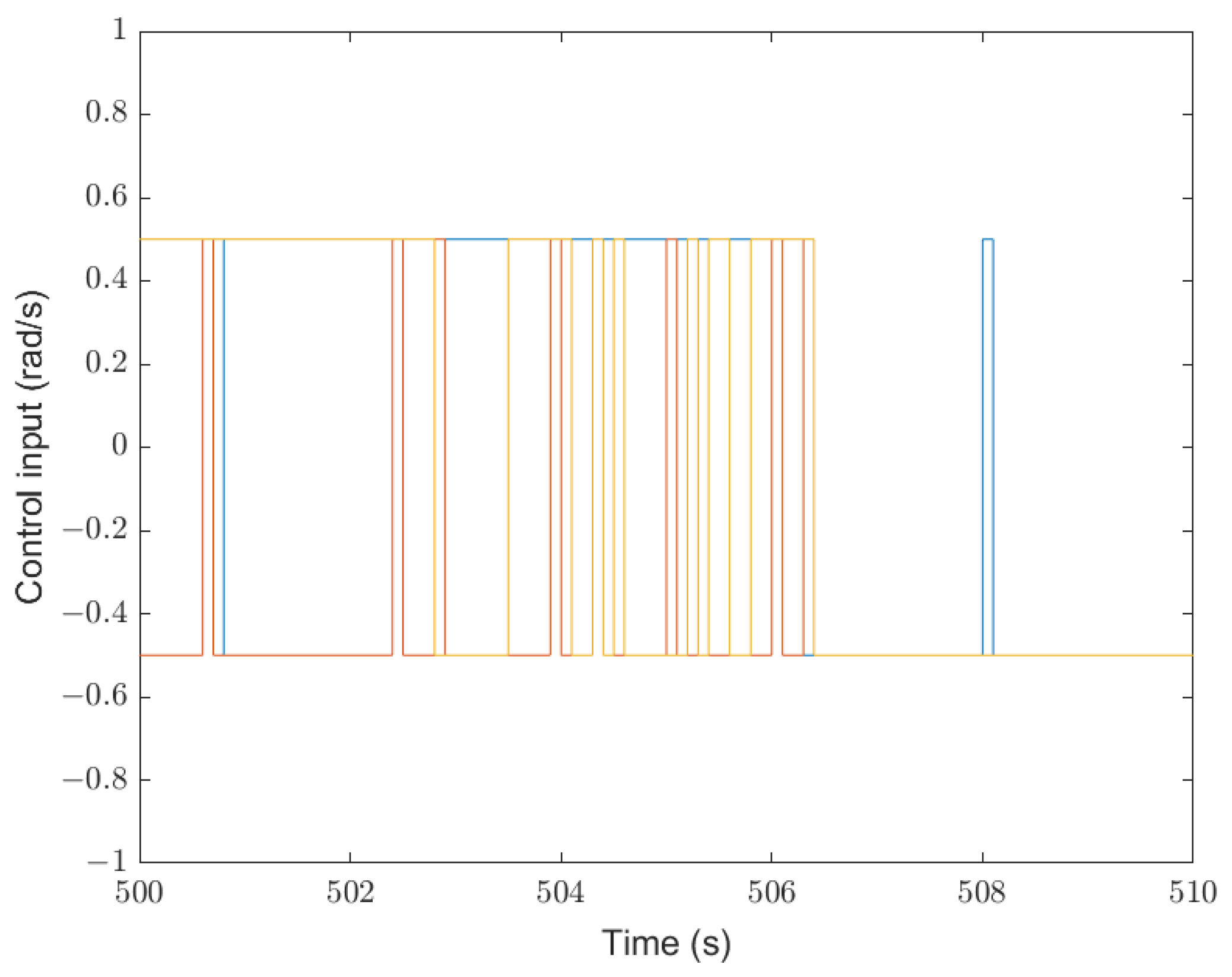
It is also important to note that while the control input can only be one of two values, the vehicles do not move in perfect circles every time. This makes sense as the control law is calculated every 0.1 s. For example, if in the period of 2 s the inputs were always the opposite of the previous one, the end result would have been something very similar to a straight line.

In Figure 9, the control input sequence for all UAVs is presented in a small excerpt of the simulation. The control input is, as can be expected, very erratic, and changing values very quickly, from the positive to negative end of the spectrum. Measures to try and overcome this issue were studied in Section 3.3.4

Some controllers can control a UAV solely given a reference turn rate, as it is very easy to translate to a roll angle reference in a fixed-wing UAV. Regardless of the controller, any reference input would be hard to follow due to the discontinuities of the reference. This is not the only drawback, of course. Given the way the input is defined, the servos in any aircraft would need to be constantly changing their positions from one extreme to the other, leading to a reduced vehicle lifespan, higher maintenance, and lower endurance due to constant use of the servo motors.

In regards to the metric for uniform coverage in Figure 10, the first thing that needs to be said is that the graph is normalized against the metric in the starting point, $\mathrm{\Phi }(t=0)$. This makes it easier to compare the metric data against other models and variables, as the starting metric is decided by the size of the domain, the risk function, and the initial vehicle positions.

In terms of the shape of the graph, it is clear the function is not monotonous. That would be impossible using this uniform coverage algorithm. On average, the metric appears to decrease exponentially in Figure 10a. This result is in line with the results obtained in [18], so it can be concluded that there was not any anomaly in the application of the algorithm when changing the model.

The noise has clear peaks which immediately decrease, almost in a recurring fashion. This is the result of the time average being used. This is better explained when thinking of a uniform distribution in the entire domain. Even if the algorithm was perfect, and the distance between the functions was 0, the next movement of the UAV would increase the distance between the distributions, and it would only reach 0 again once the rest of the domain was visited.

While the metric for uniform coverage is important, the shape of the obtained distribution is even more so. In Figure 11, the desired distribution and the obtained distribution are compared. The values do not perfectly align with the values from Figure 5, the distribution pre-Fourier Transform, but overall the different risk zones can be differentiated in the image.

3.3.1. Effect of the Number of Harmonics in the Computational Time

The process of running the simulations can be divided into two different stages: The setup stage, in which the Fourier coefficients of the desired distribution ${\mu }_k$ are obtained, as well as defining the initial conditions, and the simulation stage, where the Simulink model is run.

The number of harmonics used is directly related to computation time, both in setup and in simulation. For the setup stage, each harmonic adds two 2D integrals, one for the denominator and one for the numerator in (50). For the simulation, each harmonic effectively adds one state, which means one additional integral.

In Figure 12, the results for the computational time using different values of K are shown. The increase in computational time in the setup stage is linearly related to K, which is surprising because the number of harmonics is equal to ${(1+K)}^2$. This means that increasing the maximum number of harmonics is not such a detriment to computational time. The same can be said to the time it takes for the simulation to run, even if there is a slight inconsistency on the lower number of harmonics. This can be attributed to the way Simulink calculates the integrals, which depends heavily on threshold values and numerical precision.

3.3.2. Effect of the Constant Speed and Heading Turn Rate

In order to see how the basic parameters affected the metric, the simulation was run for different values of each of the parameters. Values from $V=20$ m/s to $V=30$ m/s were tested, as well as values from $u=0.5$ rad/s to $u=1$ rad/s. The results are shown in Figure 13.

The obtained results were very similar. There were no drastic differences in the metric for uniform coverage’s behavior, only that with each increment added to each variable, the averages seem to decrease slightly. This is more evident in the case of the linear speed.

In conclusion, the higher the linear speed and/or heading turn rate, the better the results. This is to be expected, of course, as with a higher linear speed, more of the domain can be covered in a shorter time span.

In the case of the heading turn rate, it can be concluded that a higher rate is better, as the minimization of the Hamiltonian was given for the bounded control input and the control law is directly proportional to the boundary values. The higher the absolute value of the maximum heading turn rate, the more negative the derivative of the metric for uniform coverage is allowed to be, resulting in a better performance.

Ultimately, the values for the linear speed and heading turn rate will be determined by the maximum the selected vehicle is able to provide.

3.3.3. Effect of the Number of UAVs

The difference in the number of UAVs used in the simulation is very impactful.

In Figure 14 the results for varying the number of aircrafts between 1 and 5 in terms of the metric for uniform coverage are shown.

3.3.4. Regularization of the Control Input

Invariably, increasing the number of UAVs increases the decay rate of the metric, although it is clear that there are two different groups of results, $N=1,2$ and $N=3,4,5$. The clear difference between the results can be attributed to the area of the domain in combination with the speed at which the UAVs are allowed to move. The results clearly show that the difference in the metric between 2 and 3 UAVs is considerably bigger than the difference between 3 and 4 UAVs. It can be concluded that for these particular combinations of parameters, the ideal size of the fleet would be 3 UAVs, as the performance would decrease heavily with less than 3 and stay relatively the same after 3 UAVs.

The difference between the results in the second group is the height of the cyclical peaks. The higher the number of UAVs, the lesser the height of the peak. This is to be expected, as the metric is averaged over the number of aircrafts in the simulation and the cyclical increase in the metric is due to the problem constraints. The increase in UAVs also means that the frequency of the up and down cyclical behavior is higher, as more aircrafts would lead to a decrease in the time it would take to reach the minimum value in the metric for uniform coverage due to triple the coverage, even if it is average.

In order to try and solve the issue of the irregular input, the control law from (36) was modified. Instead of using the $sign$ function, a saturation function was used, so that the regularized control law is defined as follows:

$$u_j\left(t\right)=\left\{\begin{array}{cc}-u_{max}\hfill & \mathrm{if}\gamma {\beta }_j\left(t\right)\ge u_{max}\hfill \\ -\gamma {\beta }_j\left(t\right)\hfill & \mathrm{if}\left|\right|\gamma {\beta }_j\left(t\right)\left|\right|<u_{max}\hfill \\ u_{max}\hfill & \mathrm{if}\gamma {\beta }_j\left(t\right)\le -u_{max}\hfill \end{array}\right.,$$

(51)

where $\gamma >0$ is a constant to tune the slope of the linear part of the saturation function.

The constant $\gamma$ is then a parameter to be changed, however given the way the quantity ${\beta }_j\left(t\right)$ is defined in (35), it is nearly impossible to predict even its magnitude order. Furthermore, if the target distribution $\mu$ changes, or the domain changes its size, the order of magnitude of this quantity will also change because $S_k\left(t\right)$ is directly related to the Fourier coefficients of $\mu$. The ideal value for $\gamma$ would be one that would allow for the control input to be almost always in the linear zone but have its values as close to the saturation limits as possible; meaning the higher the slope, the closer to optimal the regularized control law is.

While the order of magnitude is hard to predict, the equation for ${\beta }_j\left(t\right)$, (35), resembles the equation for the metric for uniform coverage, (7), so as a first approximation, $\gamma$ was set to the inverse of the order of magnitude of the metric at $t=0$. In the particular case of this simulation, this value is $\gamma ={10}^{14}$.

The trajectory of the different agents and their regularized control input throughout the simulation is showcased in Figure 15. The most noticeable effect of this specific regularization is that the agents spend considerable time outside of the domain to be covered, even going so far as to frequently leave the extended domain. This is because the $\gamma$ parameter is too low, causing the system to not have a control input high enough to make the needed turn. With regularization at a low slope, the control input is much closer to zero than it is to the saturation point, which would be the optimal control input. This can be seen in Figure 15b, where the control input is now always smooth and rarely ever goes above $0.2$, when the saturation point is $0.5$. The values in the saturation zone are not due to the regularization but to the method employed to keep the agents inside the extended domain.

With poor results for the trajectory, it is expected that the obtained metric for uniform coverage is also inferior when compared to the optimal result in Figure 10. This is evident from Figure 16, with the normalized metric never dropping below ${10}^{-3}$ when the optimal result almost reaches the ${10}^{-4}$ values.

In order to try to improve this, the slope was increased to $\gamma ={10}^{15}$ because there was still the option to do so, with the control input being so far from the saturated values.

The trajectory result for this value of $\gamma$ is showcased in Figure 17a, and it seems that the agents spend considerably less time outside of the domain to be covered, even if it is longer than if the input was optimal, and can still leave the extended domain. The regularized control input for the simulation is showcased in Figure 17b, and it can be seen that it reaches the saturation values very often, meaning that increasing the value of $\gamma$ would only make it so the control input saturates more often, which would defeat the point of adding saturation.

Regarding the metric for uniform coverage, shown in Figure 18, the values dropped below the ${10}^{-3}$ mark, but were not quite as low as the ones obtained from running the simulation with the optimal control law, as shown in Figure 10. Therefore, the proposed regularization fixes chattering of the input signal but exhibits some degradation in the performance. It would be counter productive to increase the value of $\gamma$ any more, as it would saturate more often and defeat the purpose of its implementation in the first place.

Furthermore, the metric is very sensitive to changes in $\gamma$ but there is no formula that can generate the ideal $\gamma$ value. The values used were obtained after analyzing the initial metric, but the metric’s order of magnitude depends on the number of harmonics used, the risk function, and the domain size. To obtain the ideal $\gamma$ value, extensive experimentation is required on a case-by-case basis.

3.4. Adapted Dubin’s Vehicle Model

When the Adapted Dubin’s Vehicle Model is introduced in Section 2.2.2, the conclusion that the y coordinate of the point in the body frame ($d_2$) does not affect the determinant of the final matrix is very important, as it can be set to zero and the system will still work perfectly fine. As such, with this $d_2$ value, the point is always situated in the $xx$ axis of the body frame.

For this simulation, the base speed of the vehicle was set to $v_b=30$ m/s and its maximum heading turn rate was set to $u_{max}=0.5$ rad/s, which are the same values used in the previous simulation.

For the values specific to this model, the distance $d_1$ was set to 2 m, and the speed differential was set to $\delta v=5$ m/s. The effects of varying the distance of the point will be studied further into this work, in Section 3.4.1.

Choosing the value for $\delta v$ needs to be done carefully because it directly relates to the minimum speed of the UAV. In this case, the minimum speed would be $V_{min}=v_B-\delta v=25$ m/s. The value $V_{min}$ needs to be above the aircraft stall speed. The time span of the simulation was, again, one hour, $T=3600$ s.

Simulating three UAVs using this model produced the trajectories in Figure 19, with the different colored lines depicting the different UAVs.

The trajectories still have an acceptable shape, without any sharp edges, unobtainable in the model. With the chosen parameters, the UAV stayed inside the extended domain and was never forced inside the domain with a non-optimal input.

The density of the lines also clearly shows the difference in surveillance time between the different areas on the domain, with the top right being the densest zone, corresponding to the area with the highest Fire Hazard Risk.

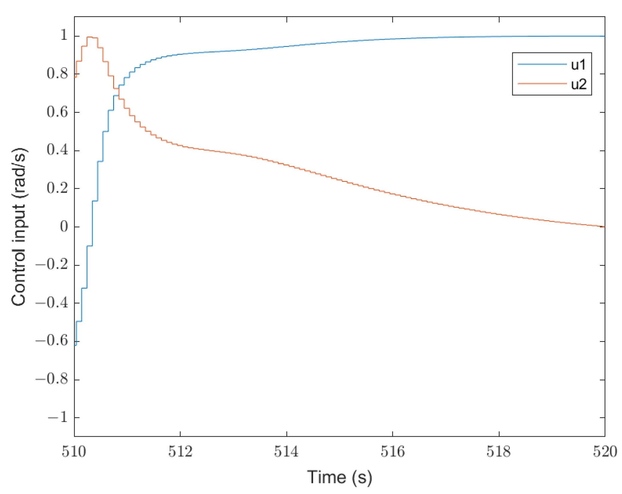
A small sample of the control input for one UAV over the course of 10 s is shown in Figure 20. The control input is smooth, even if the plot chosen was a stairs function instead of the regular plot to account for the discrete solver used.

Given that $u_2$ represents the heading turn rate, it is easy to see why the input would result in trajectories that are very easy to follow by a fixed-wing UAV. These values are small for the most part, with the transition being slow. It does not have the steep transitions from the previous model and so there should not be any agility imposition in the UAV, meaning a wider variety of aircrafts can be picked for usage.

The evolution of the metric for uniform coverage in this simulation, shown in Figure 21, exhibits an exponential behavior in logarithmic scale, confirming that the system is working as expected. The result is, once again, not a monotonous function but decreases on average as the simulation time increases.

The metric once again shows cyclical behavior after an initial transitory period, likely due to having covered the higher weighted Fourier bases, the lower frequency ones.

The heatmap of the probability density function obtained at the end of one hour of simulation is shown in Figure 22. The heatmap shows that the Very High and High areas were appropriately covered, even if the edges of the High Risk zone do not exactly have the desired shape, at around $\mathbf{x}={[1500,2000]}^{\top }$.

The Moderate areas, on the other hand, are considerably messier, with the obtained distribution having plenty of darker blue spots, associated with a Reduced classification. The edges can clearly be noticed, however the content is not entirely uniform. This is a case where a slightly higher simulation time would be very beneficial, as the finer details only get worked on after the first basis converges to acceptable results due to the weighting.

The shape of the surveillance square domain is also very blurry, due to the vehicle spending a considerable amount of the beginning of the simulation doing a short sweep on the extended domain. This is due to the parameters of the system, and will be discussed next.

Overall, the obtained result is still well within the acceptable domain. Even if the shapes are not perfectly defined and uniform in detail, it is clear the higher risk areas are being surveilled appropriately and the rest would, with a higher running time, converge to desirable uniformity.

3.4.1. Effect of Parameter Variation

The system has one defining characteristic that makes it so multiple inputs are allowed, and that is the tracking of a point on the body frame and not the center of the body frame itself.

As a result, the position of the point directly influences the amount of control over the UAV. While the control of the linear speed differential is important, it is inevitably the behavior of the heading turn rate input that makes the trajectory.

The control input component related to the heading turn rate is the second column of matrix ${\mathbf{M}}_2$, which is directly proportional to $d_1$, the x coordinate of the point in the body frame. As a result, the closer to the origin, the less effect the control law equation will have on the heading turn rate component due to the input vector being unitary. If the vector norm of the columns of ${\mathbf{M}}_2$ is very different, one component will have a bigger weighting.

In conclusion, it is better if $\delta v$ and $d_1·u_{max}$ are close, or at the very least in the same order of magnitude.

To exemplify the lack of control, the same simulation was run, however for $d_1=0.5$ m instead of the previous 2 m. The resulting trajectory is shown in Figure 23, and it is clear that the behavior is completely unacceptable.

Before any further analysis, Figure 23b shows the UAV going outside the extended domain, applying the second fail-safe measure of forcing the aircraft back inside. This figure proves the designed algorithm is working properly.

Both simulations use the same parameters, however have a different distance, with $u_{max}=0.5$ rad/s and $\delta v=5$ m/s. To expand on the previous concept of similarity in values, the product between the heading turn rate and the distance is, in the case of simulation (a) $d_1·u_{max}=1$ and $d_1·u_{max}=0.25$ for simulation (b). Comparing both of these values to the value of $\delta v$ makes it clear why the parameter is not at all well chosen. In this case, for there to be a significant change in the control input related to the turning rate in (b), the value in the multiplying vector from the control law would need to be much higher than the value related to the velocity due to the normalization of the vector.

The result of the bad choice of parameter is clear from Figure 23b, in which the UAV has difficulty turning and is less agile. The effective consequence of bad parameterization is almost an attenuation in the turn rate, which explains the wider curves produced by the model.

The direct effect of a bad trajectory was translated to the metric for uniform coverage, shown in Figure 24. While the graphs look similar at first glance, the order of magnitude on the $yy$ axis is of note, as the value in (a) is almost an order of magnitude lower than that of (b).

This figure shows that, while the control law still works for bad parameterized systems, the metric for uniform coverage would stabilize at a higher value. All the results shown up to this point suggest there is a point after which the metric for uniform coverage starts decaying at a much slower rate. The results from Figure 24 suggest that this point is influenced by the freedom the UAV is afforded on the model, something that was never previously showcased in this work. In this case, while the metric is still low, the obtained trajectory is not acceptable. In conclusion, a decrease in the metric for uniform coverage, while necessary, is not sufficient to ascertain if the model is well parameterized or not.

While a bigger distance can mean better results, it can not be so distant that it does not make sense to calculate the distribution on an unrealistic point nor should it overpower the velocity component, as the input would quickly depreciate into a graph similar to the Dubin’s Path as $u_1$ would be reaching zero after normalizing.

3.5. Model Performance Comparison

Since both the previous models had the same initial condition, same domain, and same risk function, it is possible to overlap the metric for uniform coverage graphs.

In Figure 25, the two metrics are overlapped and look very similar. The Dubin’s Vehicle model has a slightly lower average value, but the results could have easily been passed as each other’s, as they have no noticeable differences. With no noticeable differences in performance, it is up to a matter of preference as to which model to use.

The Dubin’s Path model is very simple to parameterize. Every parameter that the model has, the adapted model has as well. On the other hand, the control input is not smooth and can lead to issues with the aircraft and possibly bring difficulty in the control of the aircraft.

The Adapted Dubin’s Path model has the flexibility of having more parameters and it is not out of the realm of possibility that there is some combination of values that would perform significantly better than the Dubin’s Path mode, although none were found during the development of this work.

The biggest difference between the two models is then the fact that the control input in the Adapted Dubin’s Model is smooth. This is exactly the issue that needed to be solved and the reason this model was applied, and the fact that there is no drop in performance is a positive aspect of the Adapted Dubin’s Vehicle model.

4. Designing the Probabilistic Model for Detection

4.1. Ignition Definition

In order to estimate the probability of detection of an ignition during a surveillance mission, it is important to define what is to be considered an ignition.

For the purpose of this work, an ignition is to be the precursor to an uncontrollable fire, a small flame that might be contained easily and in a timely manner. With the most common fire causes mentioned in Section 1.1, this can be associated with a Crawling or Surface fire.

A Crawling or Surface fire is, as the name indicates, a fire caused by the burning of ground level vegetation and other fuels such as grass, trash debris, and pieces of wood from surrounding trees.

Surface fires burn at a temperature lower than crown fires, meaning fires in tree canopies, and spread slowly compared to the other forms of more intense fires. These burn with a surface temperature of around 400 °C to 500 °C, however sloped terrain and strong wind can speed up the spread of the fire [33].

Knowing the temperature at which a surface fire usually burns is extremely useful, as it can be used to estimate the power and the radiating power of a fire and thus select the most appropriate equipment to detect it.

Let an ignition then be defined as a surface fire burning at 500 °C with a small area. The area can be changed according to further studies of the fire spread inside the covered zone, so as to determine how big or small a surface fire can be before it spreads and becomes uncontrollable. For the purpose of this work, an area of 5 square meters was chosen.

Infrared (IR) sensors often function within certain wavelengths. As such, choosing between the different bands is crucial.

All blackbody matter in thermal equilibrium emits electromagnetic energy following Planck’s Law, which describes the Radiance of the energy as a function of the matter’s absolute temperature for each wavelength [34]. The radiance can be seen as the portion of total power emitted at a certain wavelength.

In Figure 26, the radiation curves for temperatures associated with fire, from around 600 K to 1400 K [33]. It can be seen that low temperature sources have their peak radiance at a wavelength of around 10 $\mathsf{\mu }$m, while sources such as fire have their peak radiance between 2 and 5 $\mathsf{\mu }$m.

In [34], it is stated that experimental evidence supports the assumption that in the Thermal Infrared Range (TIR), between 0.75 and 15 $\mathsf{\mu }$m, fire radiation can be modeled using Planck’s Law despite not being exactly a blackbody.

Using TIR sensors is extremely useful due to the fact that they only detect the radiation power of certain wavelengths and as such ignore most of what could limit visibility, such as trees and thick smoke. In the case of fire detection, Medium Wavelength Infrared (MWIR) Sensors are exactly what is needed. MWIR sensors work in wavelengths between 3 and 8 $\mathsf{\mu }$m [34]. Incidentally, the energy radiated peaks inside that range, and the sensor will ignore lower temperature readings due to them being outside of the wavelength bounds imposed by the sensor.

Average Power Radiated by an Ignition

The power emitted by a fire source is extremely complicated to estimate. The more complete models have multiple specific parameters and very complex equations. For the purpose of this work, the simplest model for the flame power will be used, as it is accurate enough to provide results that are not completely unrealistic. Consequently, the power radiated by a flame will be estimated with the Stefan–Boltzmann law, one of the simplest models which estimates the power radiated by a blackbody [35]. This power is a function of the source’s temperature and body area, hence the importance of the values gathered previously.

The Stefan–Boltzmann law is given by the following expression,

$$P(T,A)=\sigma A{T}^4$$

(52)

where $\sigma =5.670374419\times {10}^{-8}$ W·m${}^{-2}$·K${}^{-4}$ is the Stefan–Boltzmann constant, T is the body’s absolute temperature, and A is the body’s radiating area.

With the temperature of T = 752.15 K (500 C) and a surface area of $A=5$ m${}^2$, an ignition radiates the following power in the surface, $P_{0i}$:

$$P_{0i}=1.0131\times {10}^{5}Watts$$

4.2. Probability of Detection

Out of every measure already mentioned throughout this work, none is more important than the probability of detection of an ignition. A high probability of detection means the network is functioning as intended and the odds of having an uncontrollable catastrophe are reduced. It is then of extreme importance that said probability is maximized. For this reason, there needs to be a model for the probability of detection when employing the Aerial Sensing Network.

The simulations performed in Section 3 provide the average probability density function for the position of any of the UAVs in the Aerial Sensing Network. This is the function $C^t$ in (1). The function is constantly changing throughout the simulation, so it is important that an opportune moment is chosen to calculate the probability of detection over a mission. This is the last obtained value of the function, obtained using the Fourier Coefficients and the Fourier basis function in (4). An example of this would be the probability density function in Figure 22b.

Let a UAV position $(x_v,y_v)$ be a point in the coverage domain U. With the last moment of the simulation taken into consideration, the probability density of at least one UAV in the network being in $(x_v,y_v)$ is $P_v(x_v,y_v)$, defined as:

$$P_v(x_v,y_v)=C^{t=3600}.$$

(53)

The probability density function of an ignition is the target distribution function of the algorithm, $\mu$. As such, let $(x_i,y_i)$ be a point in the coverage domain U. The probability of an ignition happening in $(x_i,y_i)$ is $P_i(x_i,y_i)$, defined as:

$$P_i(x_i,y_i)=\mu (x_i,y_i).$$

(54)

Lastly, the probability density function of detection of an ignition in $(x_i,y_i)$ by a UAV in $(x_v,y_v)$ needs to be defined. This is the sensor model.

4.2.1. Sensor Model

The model for the probability of detection depends entirely on the sensor used. However, it was not feasible to obtain any sort of sensor for this work to model said probability. Every sensor is different and the modern sensors also have a different performance depending on the software used to process the images obtained.

The objective is to provide a general workflow to test and parameterize the UAV fleet before the full ASN is deployed. Consequently, a general sensor model is used as an example to generate data. In a real work environment, this is the step that would require further fine tuning in the form of obtaining the sensing effectiveness of the sensor used in conjunction with the image processing software.

The model used for this part was proposed in [36] and takes advantage of the fact that electromagnetic radiation propagates spherically in a vacuum and in a free medium such as air. The result of this is that the power dissipation is proportional to the inverse of the distance traveled squared. As such, the noisy measurement obtained by the IR sensor can be modeled by the following equation,

$$P_r(x_v,y_v,x_i,y_i)=\frac{P_{0i}}{4\pi R{(x_v,y_v,x_i,y_i)}^2}+n_{i}Watts$$

(55)

where the parameter $n_i$ is a random variable following a Gaussian distribution and $R(x_v,y_v,x_i,y_i)$ is the distance between the ignition point and the sensor position, which is the vehicle position, given by:

$$R(x_v,y_v,x_i,y_i)=\left|\right|(x_v,y_v,h)-(x_i,y_i,0)\left|\right|$$

(56)

where h is the flight altitude of the vehicle, a constant parameter over the surveillance mission.

The proposed model for the probability of detection is based on whether the power received by the sensor is higher than a certain threshold. Consequently, let $P_{sens}(x_v,y_v,x_i,y_i)$ be the probability of the sensor at $(x_v,y_v)$ detecting an ignition at $(x_i,y_i)$ be given by the the following expression:

$$P_{sens}(x_v,y_v,x_i,y_i)=\{P_r(x_v,y_v,x_i,y_i)>c\}.$$

(57)

The important variables to determine for this model are then the standard deviation of the white noise added to the received power and the threshold at which a detection is deemed to have failed.

These parameters would change considerably for each different sensor and software combination used. However, for the purpose of this work some values were estimated in order to showcase the paremeterization workflow.

The threshold c is the first to be decided. To obtain this value, a distance from the ignition at which the sensor has a 50% chance of detection needed to be chosen. The various aircrafts compiled in Table 2 show that missions at 5000 to 6500 m above sea level are possible, so it is assumed that the sensors would work at that range.

The value chosen for the 50% detection mark was then 5000 m. This value could easily be changed to accommodate a specific sensor. The threshold for the used sensor model is then:

$$c=\frac{P_{0i}}{4\pi {5000}^2}=3.2247\times {10}^{-4}Watts.$$

(58)

The standard deviation, however, is a much more complex number to estimate. It directly affects the shape of the probability function. It can be interpreted as a combination of a sensor noise, sensor resolution, software effectiveness, and even further power losses due to an imperfect medium with the presence of smoke and foliage.

The cumulative normal distribution has a sigmoid function shape, which means the sensor probability function does as well. The magnitude of the standard deviation could not be much lower than ${10}^{-4}$, the magnitude of the threshold, as it would turn so that the probability function would have a slope steep enough to almost be a step function, 1 before 5000 m and 0 after 5000 m. The value chosen for the standard deviation is $\sigma =5\times {10}^{-5}$ and makes it so there is a decrease of detection probability from 0.9 to 0.1 from around 4500 m to 5500 m, which a much more realistic behavior. This value is of course easily adjustable by testing the IR sensor in use.

In Figure 27 the probability of detection of an ignition is plotted in function of the distance to the sensor, with a threshold c and additive noise $n_i\to \mathcal{N}(0,{\sigma }^2)$.

Not only are the sensors limited by distance, they are also limited by their field of view. To take into consideration the FOV of the sensor, it will be assumed that the sensor is always pointing straight down from the aircraft and has a conic field of view. The radius of the cone on the ground can then be written as follows,

$$r=h\arctan \left(\frac{\gamma }{2}\right),$$

where h is the flight altitude and $\gamma$ is the angle of the cone of view. This angle can range between different values even in the same sensor, however as it increases, the resolution of the obtained image also decreases due to more area being covered with the same amount of pixels. The value used throughout this section is $\gamma =$ 24°, a value that sits in the middle of the range in sensors such as [37].

The value of $\gamma$ can be changed depending on the circumstances. In a more complete model, $P_{sens}$ would have a component that depended on this angle and it could be used as a parameter for optimization. However, with the lack of a physical sensor for testing, this was not achieved.

Ultimately, the sensor model to be used is $P_s$, defined as follows,

$$P_s(x_i,y_i,x_v,y_v)=\left\{\begin{array}{cc}{P}_{sens}(x_i,y_i,x_v,y_v)\hfill & \mathrm{if}\left|\right|(x_i,y_i)-(x_v,y_v)\left|\right|\le r\hfill \\ 0\hfill & \mathrm{otherwise}\hfill \end{array}\right..$$

(59)

4.2.2. Probability Function

With a well-defined sensor model, vehicle position probability density function, and ignition probability density function, the overall probability of one UAV in the network detecting an ignition can be the integral of the product of those three over all possible vehicle and ignition positions,

$$P_d={\int \int }_U^{}{\int \int }_U^{}{P}_s(x_v,y_v,x_i,y_i)P_i(x_i,y_i)P_v(x_v,y_v)d{x}_{v}d{y}_{v}d{x}_{i}d{y}_i$$

(60)

with domain U defined in Section 3.1.2.

The detection of an ignition is an independent event for each aircraft in the network, and as such, for the whole network, the important measure is the probability of at least one aircraft detecting the ignition. That is the complementary probability of none of the UAVs detecting the ignition. Consequently, for a network of N UAVs, the joint probability of detection is given as:

$$P_{joint}=1-\prod _{i=1}^N(1-P_d).$$

(61)

4.3. Parametric Study

In order to apply the probability functions from Equations (60) and (61), the Simulink simulation for the Adapted Dubin’s Vehicle model was used. The data extracted from the simulation were the final Fourier coefficients of the agent average position probability function in order to build the function from (53).

The parametric study from this section has the end goal of aiding the user in choosing the right number of agents for the surveillance network. With an approximated probability of detection, the overall cost of the network, including buying the UAV, their surveillance software and maintenance can be balanced out by the expected economical damage that a fire would cause. It would then be up to the user to decide how many UAVs to buy and at which altitude the surveillance mission would take place at.

4.3.1. Influence of the Flight Altitude

The altitude of the agents is not evident just by analyzing the equations. While a decrease in altitude would mean the sensor is more likely to detect an ignition, it also means that it is covering less area at once due to the FOV restrictions.

To clarify the effect of the flight altitude, the probability density function for the average position of the UAVs ($P_v$), shown in Figure 22, for a network of 3 agents, and the probability density function for the ignition location ($P_i$), shown in Figure 5.

In Figure 28, the results for flight altitudes from 500 m to 5500 m are shown. The probability of detection shows a clear peak at an altitude of 4500 m.

The most important conclusion to take from this graph is that the sensor model is a limiting factor in the detection probability due to both range limitations and FOV restrictions. Considering these restrictions, there is an optimal flight altitude, in this case being somewhere close to 4500 m.

The increase in the probability of detection until the 4500 m altitude mark is explained by the FOV restrictions. At that altitude, the distance between the sensor and the ignition would almost always be inside the region where the probability of detection is near 1 in Figure 27. Increasing the altitude in those ranges increases the area covered by the agents at any given time, thus increasing the probability of detection.

There is a sharp decrease in the probability of detection at the 4500 m mark, which is the distance at which the sensor probability of detection is around 90%. By design of the model, after that distance, the sensor performance starts decreasing rapidly, with a detection probability of around 10% at 5500 m. This is important because the flight altitude is the minimum distance at which the sensor would be able to sense the ignition, and it would happen when the aircraft would be positioned directly upwards of the ignition. Consequently, the maximum flight altitude is directly affected by the sensor used and in this case, anything above 4500 m makes little sense.

4.3.2. Influence of the Number of Agents

The number of agents in the ASN has an effect not only in the joint probability of detection (cf. (61)) but also on the final probability density function for the average position of each agent ($P_v$), a direct result of the data shown in Figure 14. One of the conclusions taken from that last figure was that increasing the number of agents would take the obtained probability density function of the vehicle position closer and closer to the target function, which is the probability density function function of the ignition location ($P_i$). Consequently, it is unexpected and improbable that increasing the number of agents decreases the individual probability of detection. However, this test is ideal to test the effect of small deviations from the target distribution in the context of the probability of detection.

To obtain the different $P_v$ functions, as it change slightly with the number of UAVs in the simulation, the same simulation used to obtain the probability density function shown in Figure 22, using the Adapted Dubin’s Vehicle mode, was run however the number of UAVs in the simulation were changed to a range of $N=1$ to $N=6$.

The results obtained are shown in Figure 29, with the probability of detection of the ASN at a flight altitude of h = 4500 m. The values for the individual probability of detection stayed almost the same for every simulation, with deviations smaller than 0.5% in magnitude. This is explained by the results in Figure 14. The metric for uniform coverage tended to decrease faster the more agents in the network but the end result was still in the same order of magnitude, so the performance was, in practice, very similar. In a probabilistic model where the most limiting factor is the sensor performance, the small difference in performance has little to no impact.

Even if the minute changes in the $P_v$ function between the simulations do not affect the individual probability of detection, the joint probability of detection increases with the number of agents, but can quickly reach the saturation point of 1 due to the nature of Equation (61).

How quickly the value of the joint probability reaches the saturation depends on the value of the individual probability of detection. In Figure 30, various values for a base individual probability of detection were utilized to showcase the increase over the base value that occurs when adding more UAVs. This is unrelated to Figure 29 and is only to serve as a showcase to the difference in the effectiveness of adding another agent for different probability values.

The effectiveness of adding more agents increases as the probability of detection by each agent decreases. For example, adding a third UAV to the network if the probability of detection of the individual UAV is 80% would barely add value to the ASN. On the other hand, if each UAV has an individual probability of detection of 20%, adding the other four increases the value of the joint probability detection by almost 250% over the base value of 20%, to a joint probability of detection of 70%.

4.3.3. Influence of the Domain Area

The size of the domain is something that has not yet been studied in this work. That is because the scalability of the uniform coverage algorithm when the domain scale is concerned was never in question. The equations for the optimal control law never depended on the domain size. In fact, most of the values used in the calculations were normalized.

To introduce domain scaling, a Domain Scaling Factor scalar value is used. This value is used to scale the domain covered as a proportional factor that multiplies the risk function in Figure 5. For example, for the base domain of $2000\times 2000$ m, a factor of 4 means the area to be covered is then $8000\times 8000$ m with a risk function with the exact same shape as the one in Figure 5.

The results of varying the scaling factor between 1 and 4 are shown in Figure 31. The flight altitude considered is $h=4500$ m, the optimal altitude from Figure 28 and for an ASN of 3 UAVs.

The decrease in the probability of detection as the domain size increases is very sharp. It is important to note that because the scaling factor scales the width and length of the domain, the area increase is actually the scaling factor squared. For the domain factor of 2, the area to be covered is $2^2=4$ times as big. The shape of the individual probability of detection is reminiscent of half a parabola, which is understandable considering the area factor is the domain scaling factor squared. In conclusion, while not an exact relation, doubling the area covered the results in about half the individual probability of detection.

In order to preserve a high joint probability of detection as the domain scale goes up, an increasing number of agents is needed to properly cover the area. For example, for the scaling factor of 4, 20 agents would be needed to obtain a joint probability of detection of 64.75%.

4.3.4. Parametric Study Conclusions

There are two main conclusions to take from the parametric study:

• The resource allocation problem was solved using the uniform coverage algorithm;
• The area coverage problem is entirely limited by the sensing method.

The first conclusion is proven by the results in Figure 29, which combined with the results from Section 3, show that the resources were allocated to higher risk zones independently of the number of agents in the ASN. In fact, the addition of more agents did not change their own individual detection probability in any considerable way because for any of the tests, the probability density function for the agent positions obtained by the uniform coverage algorithm was already very close to the desired distribution. The bottle-neck of (60) for the individual probability of detection is the sensor function $P_s$.

For the most part, the most important graph is shown in Figure 28 which, when looked at in tandem with the rest of this section, can be the defining factor for the final parameterization of the ASN. The peak probability of detection is right before the heavy decay from the sensor model, particularly with the threshold of 50% chance of detecting the ignition at a distance of 5000 m. Getting a better sensor, both in terms of software and hardware, can increase this threshold, which is extremely valuable as the threshold is the definitive bottle-neck of the probabilistic model. Before the peak at $h=4500$ m, the probability of detection was increasing almost linearly, so it stands to reason that should the threshold be increased, the linear increase would keep happening until the new threshold value took effect.

With a higher individual probability of detection, fewer UAVs need to be deployed and larger domains can be covered for a cheaper price. From the data in Figure 30, the increase in performance of the ASN by increasing the amount of agents can be obtained and balanced against the cost of the new agent. Given the nature of the risk distributions being associated with economical damage, each percentage point in the joint probability of detection can be associated with a monetary value. Adding another UAV becomes non-profitable when the performance increase of adding it results in a percentage increase in detection that has an inferior monetary value compared to the cost of the UAV and its maintenance.

5. Conclusions

Overall, the objectives outlined in Section 1.3 were all properly accomplished throughout this work. In Section 2, the theoretical basis for the algorithm was established, with all the functions defined for understanding how to say if the trajectories of the system can be considered uniform. In light of the movement restrictions of a fixed-wing UAV, two different movement models were introduced in Section 2.2.1 and Section 2.2.2 that are easily associated with the coordinated turn movement of an aircraft. The model in Section 2.2.1 has a scalar control input while the model in Section 2.2.2 has a two dimensional control input. By the end of Section 2, the optimal feedback control laws for both models were obtained.

In Section 3, the Fire Hazard Risk function was defined in order to run Matlab/Simulink simulations for both models. In this Section, the issue of the agents being able to leave the domain due to the symmetry in the Fourier Transform were taken into consideration and solved by extending the Fourier Transform domain and forcing the agent back inside should it leave.

The results of the simulation for the Dubin’s Vechicle Model in Section 3.3 showed that the metric for uniform coverage converges to nearly zero, and the heatmaps of the probability density function of the UAV position closely resemble the desired heatmap. There is an issue due to the one dimensional nature of the control input, which can be solved by a regularization at the cost of some performance.

The results of the simulation for the Adapted Dubin’s Vehicle Model in Section 3.4 show that the performance is equivalent to the performance in of the Dubin’s Vehicle Model before regularization without having issues in the control input. However, the model is very sensitive to bad parameterization, which can cause the model to not function properly if the parameters are not picked carefully.

In Section 4.1, the concept of ignition was defined in order for a probabilistic model for the ignition detection probability to be proposed. A sensor model for a Infra-Red sensor was proposed and is the basis for the probabilistic model.

Lastly, the workflow to decide how to size the sensing network was proposed, studying the effect of different parameters, such as flight altitude and the number of UAVs. It was concluded that the sensor model was the bottleneck of the probability of detection, namely the conic angle that defined the FOV and the distance from the ignition at which the sensor starts losing performance. Additionally, due to FOV restrictions, there is an optimal altitude for the ASN that maximizes the joint probability of detection.

References

1. Departamento Gestão de Áreas Públicas e de Protecção Florestal. 10° Relatório Provisório de Incêndios Florestais; Instituto de Conservação da Natureza e das Florestas: Lisbon, Portugal, 2017. [Google Scholar]
2. Pinto, L. Pedrógão Grande: Governo Estima Prejuízos de 500 Milhões de Euros. 2017. Available online: https://www.publico.pt/2017/07/03/sociedade/noticia/pedrogao-grande-governo-estima-prejuizos-de-500-milhoes-de-euros-1777751 (accessed on 14 October 2021).
3. San-Miguel-Ayanz, J.C.A. Forest Fires at a Glance: Facts, Figures and Trends in the EU; European Forest Institute: Sarjanr, Finland, 2009; pp. 11–18. [Google Scholar]
4. Departamento Gestão de Áreas Públicas e de Protecção Florestal. 6° Relatório Provisório de Incêndios Florestais; Instituto de Conservação da Natureza e das Florestas: Lisbon, Portugal, 2021. [Google Scholar]
5. Meira Castro, A.C.; Nunes, A.; Sousa, A.; Lourenço, L. Mapping the Causes of Forest Fires in Portugal by Clustering Analysis. Geosciences 2020, 10, 53. [Google Scholar] [CrossRef] [Green Version]
6. Emery, W.; Camps, A. Introduction to Satellite Remote Sensing; Elsevier: Amsterdam, The Netherlands, 2017. [Google Scholar]
7. Kaufman, Y.J.; Justice, C.O.; Flynn, L.P.; Kendall, J.D.; Prins, E.M.; Giglio, L.; Ward, D.E.; Menzel, W.P.; Setzer, A.W. Potential global fire monitoring from EOS-MODIS. J. Geophys. Res. Atmos. 1998, 103, 32215–32238. [Google Scholar] [CrossRef]
8. Alkhatib, A. A Review on Forest Fire Detection Techniques. Int. J. Distrib. Sens. Netw. 2013, 2014, 597368. [Google Scholar] [CrossRef] [Green Version]
9. Avellar, G.; Pereira, G.; Pimenta, L.; Iscold, P. Multi-UAV Routing for Area Coverage and Remote Sensing with Minimum Time. Sensors 2015, 15, 27783–27803. [Google Scholar] [CrossRef] [PubMed] [Green Version]
10. Thomas, D.; Butry, D.; Gilbert, S.; Webb, D.; Fung, J. The Costs And Losses of Wildfires: A Literature Survey; Technical report; National Institute of Standards and Technology: Gaithersburg, MD, USA, 2017. [CrossRef]
11. Catry, F.X.; Rego, F.; Bação, F.; Moreira, F. Modeling and mapping wildfire ignition risk in Portugal. Int. J. Wildland Fire 2009, 18, 921–931. [Google Scholar] [CrossRef] [Green Version]
12. Van Wagner, C.E. Development and Structure of the Canadian Forest Fire Weather Index System; Forestry Technical Report 35, Technical report; Canadian Forestry Service: Ottawa, ON, Canada, 1987. [Google Scholar]
13. IPMA. Cálculo do Índice de Risco de Incêndio Rural Risco Conjuntural e Meteorológico—RCM; Technical report; Instituto Português do Mar e da Atmosfera: Lisbon, Portugal, 2020. [Google Scholar]
14. Verde, J.C.; Zêzere, J.L. Assessment and validation of wildfire susceptibility and hazard in Portugal. Nat. Hazards Earth Syst. Sci. 2010, 10, 485–497. [Google Scholar] [CrossRef]
15. Lourenço, L.; Mira, M. Grandes incêndios florestais de 17 de junho de 2017 em Portugal e exemplos da determinação das respetivas causas. Territorium 2019, 26, 49–60. [Google Scholar] [CrossRef]
16. Galceran, E.; Carreras, M. A survey on coverage path planning for robotics. Robot. Auton. Syst. 2013, 61, 1258–1276. [Google Scholar] [CrossRef] [Green Version]
17. Xu, A.; Viriyasuthee, C.; Rekleitis, I. Optimal complete terrain coverage using an Unmanned Aerial Vehicle. In Proceedings of the 2011 IEEE International Conference on Robotics and Automation, Shanghai, China, 9–13 May 2011; pp. 2513–2519. [Google Scholar] [CrossRef] [Green Version]
18. Mathew, G.; Mezic, I. Metrics for ergodicity and design of ergodic dynamics for multi-agent systems. Phys. D Nonlinear Phenom. 2011, 240, 432–442. [Google Scholar] [CrossRef]
19. Michael, N.; Stump, E.; Mohta, K. Persistent surveillance with a team of MAVs. In Proceedings of the 2011 IEEE/RSJ International Conference on Intelligent Robots and Systems, San Francisco, CA, USA, 25–30 September 2011; pp. 2708–2714. [Google Scholar] [CrossRef]
20. Tokekar, P.; Kumar, V. Visibility-based persistent monitoring with robot teams. In Proceedings of the 2015 IEEE/RSJ International Conference on Intelligent Robots and Systems (IROS), Hamburg, Germany, 28 September–2 October 2015; pp. 3387–3394. [Google Scholar] [CrossRef]
21. Petersen, K.E. Ergodic Theory; Cambridge University Press: Melbourne, Australia, 1989. [Google Scholar]
22. Mathew, G.; Mezic, I.; Petzold, L. A multiscale measure for mixing. Phys. D Nonlinear Phenom. 2005, 211, 23–46. [Google Scholar] [CrossRef]
23. Beard, R.W.; McLain, T.W. Small Unmanned Aircraft: Theory and Practice; Princeton University Press: Princeton, NJ, USA, 2012. [Google Scholar]
24. Lawton, J.R.; Beard, R.W.; Young, B.J. A decentralized approach to formation maneuvers. IEEE Trans. Robot. 2003, 19, 933–941. [Google Scholar] [CrossRef] [Green Version]
25. Kirk, D.E. Optimal Control Theory: An Introduction; Dover Publications: Mineola, NY, USA, 2004. [Google Scholar]
26. PX4 Controller. Available online: https://docs.px4.io/v1.12/en/ (accessed on 14 October 2021).
27. Fixed Step Solvers in Simulink. Available online: https://www.mathworks.com/help/simulink/ug/fixed-step-solvers-in-simulink.html (accessed on 28 January 2021).
28. Albatross. Available online: https://www.unmannedsystemstechnology.com/company/applied-aeronautics/ (accessed on 14 October 2021).
29. Helvetis—Jabali. Available online: https://helvetis.com/vtol-uav-isr/ (accessed on 14 October 2021).
30. PD-2 UAS VTOL. Available online: https://www.unmannedsystemstechnology.com/company/ukrspecsystems/pd-2-uas-vtol-fixed-wing-uas/ (accessed on 14 October 2021).
31. STREAM C VTOL. Available online: https://threod.com/products/stream-c-vtol/ (accessed on 14 October 2021).
32. Bramor ppX. Available online: https://www.c-astral.com/en/unmanned-systems/bramor-ppx (accessed on 14 October 2021).
33. Scott, A.C.; Bowman, D.M.J.S.; Bond, W.J.; Pyne, S.J.; Alexander, M.E. Fire on Earth: An Introduction; Wiley-Blackwell: West Sussex, UK, 2014. [Google Scholar]
34. Allison, R.S.; Johnston, J.M.; Craig, G.; Jennings, S. Airborne Optical and Thermal Remote Sensing for Wildfire Detection and Monitoring. Sensors 2016, 16, 1310. [Google Scholar] [CrossRef] [PubMed] [Green Version]
35. Rossi, J.L.; Chetehouna, K.; Collin, A.; Moretti, B.; Balbi, J.H. Simplified Flame Models and Prediction of the Thermal Radiation Emitted by a Flame Front in an Outdoor Fire. Combust. Sci. Technol. 2010, 182, 1457–1477. [Google Scholar] [CrossRef] [Green Version]
36. Li, W.; Cassandras, C. Distributed Cooperative coverage Control of Sensor Networks. In Proceedings of the 44th IEEE Conference on Decision and Control, Seville, Spain, 12–15 December 2005; pp. 2542–2547. [Google Scholar] [CrossRef]
37. FLIR Boson. Available online: https://www.flir.eu/support/products/boson/ (accessed on 14 October 2021).
Figure 1. Illustration of a Dubin’s Vehicle trajectory and of the local coordinate frame.
Drones 06 00044 g001
Figure 2. Adapted vehicle’s coordinate frame.
Drones 06 00044 g002
Figure 3. Base risk function for simulation.
Drones 06 00044 g003
Figure 4. The Fourier Transform of the Fire Hazard Risk Distribution for K = 15 in a larger domain and the trajectories obtained by running the simulation from Section 3.3 without countermeasures for the agents leaving the domain. (a) The Fourier Transform of the Fire Hazard Risk Distribution for K = 15 in a larger domain. (b) The trajectories obtained by running the simulation from Section 3.3 without countermeasures for the agents leaving the domain.
Drones 06 00044 g004
Figure 5. Risk function with an extended domain.
Drones 06 00044 g005
Figure 6. Fire Hazard probability function and its Fourier approximation with K = 15 . (a) Fire Hazard probability. (b) Fourier Transform of the Fire Hazard probability.
Drones 06 00044 g006
Figure 7. Control scheme of a full aircraft.
Drones 06 00044 g007
Figure 8. Obtained trajectory for three UAVs (Unmanned Aerial Vehicles) using the Dubin’s Vehicle model.
Drones 06 00044 g008
Figure 9. Control input sequence for the three UAVs in t = [ 500 , 510 ] s.
Drones 06 00044 g009
Figure 10. Metric for uniform coverage representation for a one-hour simulation. (a) Metric for uniform coverage with both log scales. (b) Metric for uniform coverage with y log scale.
Drones 06 00044 g010
Figure 11. Visualization of the desired probability density function and the obtained probability density function’s heatmap. (a) Heatmap of the desired probability density function. (b) Heatmap of the obtained probability density function.
Drones 06 00044 g011
Figure 12. Effect of the number of harmonics in computational time, in the setup stage, and in the simulation. (a) Computational time in the setup stage for different values of K. (b) Computational time in the simulation for different values of K.
Drones 06 00044 g012
Figure 13. Effect of the linear speed and heading turn rate on the Dubin model. (a) Effect of the linear speed on the Dubin model. (b) Effect of the heading turn rate on the Dubin model.
Drones 06 00044 g013
Figure 14. Effect of the number of UAVs in the metric for uniform coverage.
Drones 06 00044 g014
Figure 15. Trajectory and control input obtained for the regularized control input with γ = 10 14 . (a) Trajectory. (b) Regularized control input.
Drones 06 00044 g015
Figure 16. Metric for uniform coverage for a regularized input with γ = 10 14 .
Drones 06 00044 g016
Figure 17. Trajectory and control input obtained for the regularized control input with γ = 10 15 . (a) Trajectory. (b) Regularized control input.
Drones 06 00044 g017
Figure 18. Metric for uniform coverage for a regularized input with γ = 10 15 .
Drones 06 00044 g018
Figure 19. Obtained trajectory for three UAVs using the Adapted Dubin’s path model.
Drones 06 00044 g019
Figure 20. Control input for one UAV in t = [ 510 , 520 ] s.
Drones 06 00044 g020
Figure 21. Metric for uniform coverage representation for a one-hour simulation with the Adapted Dubin’s Vehicle Model. (a) Metric for uniform coverage with both log scales. (b) Metric for uniform coverage with y log scale.
Drones 06 00044 g021
Figure 22. Visualization of the desired probability density function and the obtained probability density function’s heatmap on the Adapted Dubin’s Vehicle Model. (a) Heatmap of the desired probability density function. (b) Heatmap of the obtained probability density function.
Drones 06 00044 g022
Figure 23. Effect of the tracked point’s position in the trajectory of the Adapted Dubin’s Path Model. (a) Trajectory for d 1 = 2 m. (b) Trajectory for d 1 = 0.5 m.
Drones 06 00044 g023
Figure 24. Effect of the tracked point’s position in the metric for uniform coverage of the Adapted Dubin’s Path Model. (a) Metric for uniform coverage for d 1 = 2 m. (b) Metric for uniform coverage for d 1 = 0.5 m.
Drones 06 00044 g024
Figure 25. Comparison between the metric for uniform coverage of the Dubin’s Vehicle and the Adapted Dubin’s Vehicle.
Drones 06 00044 g025
Figure 26. Planck’s Law curves for ideal blackbody radiation at high temperatures between 300K and 1200K. Smaller wavelengths produce higher peaks.
Drones 06 00044 g026
Figure 27. Probability of the sensor detecting an ignition at a distance of R meters from the sensor.
Drones 06 00044 g027
Figure 28. Probability of detecting an ignition in the function of the altitude.
Drones 06 00044 g028
Figure 29. Probability of detecting an ignition in function of the number of agents.
Drones 06 00044 g029
Figure 30. Percentage increase over the individual probability value with the number of UAVs, for a variety of base probabilities.
Drones 06 00044 g030
Figure 31. Probability of detecting an ignition in the function of the domain size.
Drones 06 00044 g031