Next Article in Journal
A Reinforcement Learning Approach Based on Automatic Policy Amendment for Multi-AUV Task Allocation in Ocean Current
Next Article in Special Issue
A Hybrid Model and Data-Driven Vision-Based Framework for the Detection, Tracking and Surveillance of Dynamic Coastlines Using a Multirotor UAV
Previous Article in Journal
Deep Learning-Based Energy Optimization for Edge Device in UAV-Aided Communications
Previous Article in Special Issue
UAV Approach for Detecting Plastic Marine Debris on the Beach: A Case Study in the Po River Delta (Italy)
 
 
Correction published on 23 September 2022, see Drones 2022, 6(10), 274.
Article

Optimizing the Scale of Observation for Intertidal Habitat Classification through Multiscale Analysis

by
Michael C. Espriella
* and
Vincent Lecours
School of Forest, Fisheries and Geomatics Sciences, University of Florida, Gainesville, FL 32653, USA
*
Author to whom correspondence should be addressed.
Drones 2022, 6(6), 140; https://doi.org/10.3390/drones6060140
Submission received: 8 May 2022 / Revised: 3 June 2022 / Accepted: 4 June 2022 / Published: 7 June 2022 / Corrected: 23 September 2022
(This article belongs to the Special Issue UAVs for Coastal Surveying)

Abstract

:
Monitoring intertidal habitats, such as oyster reefs, salt marshes, and mudflats, is logistically challenging and often cost- and time-intensive. Remote sensing platforms, such as unoccupied aircraft systems (UASs), present an alternative to traditional approaches that can quickly and inexpensively monitor coastal areas. Despite the advantages offered by remote sensing systems, challenges remain concerning the best practices to collect imagery to study these ecosystems. One such challenge is the range of spatial resolutions for imagery that is best suited for intertidal habitat monitoring. Very fine imagery requires more collection and processing times. However, coarser imagery may not capture the fine-scale patterns necessary to understand relevant ecological processes. This study took UAS imagery captured along the Gulf of Mexico coastline in Florida, USA, and resampled the derived orthomosaic and digital surface model to resolutions ranging from 3 to 31 cm, which correspond to the spatial resolutions achievable by other means (e.g., aerial photography and certain commercial satellites). A geographic object-based image analysis (GEOBIA) workflow was then applied to datasets at each resolution to classify mudflats, salt marshes, oyster reefs, and water. The GEOBIA process was conducted within R, making the workflow open-source. Classification accuracies were largely consistent across the resolutions, with overall accuracies ranging from 78% to 82%. The results indicate that for habitat mapping applications, very fine resolutions may not provide information that increases the discriminative power of the classification algorithm. Multiscale classifications were also conducted and produced higher accuracies than single-scale workflows, as well as a measure of uncertainty between classifications.

1. Introduction

Studying intertidal habitats as intricate mosaics forming a system rather than individual patches can allow for a better understanding of the complex and dynamic interactions in these environments [1,2,3,4]. Ecosystem services provided by intertidal habitats, such as oyster reefs, salt marshes, and mudflats, are often multifaceted as services may be amplified or hindered by patch configuration. For example, the presence of the Crassostrea virginica (eastern oyster) shell adjacent to a salt marsh can reduce erosion [5], the composition and spatial configuration of intertidal habitats can affect the community structure [6,7], and denitrification services provided by oyster reefs are dependent on habitat context [8].
Traditionally, sampling these environments has been very cost and time-intensive, often relying on in situ approaches that do not provide a full picture of the ecosystem. Remote sensing alternatives provide an opportunity to reduce costs while still capturing valuable information about habitat coverage and configuration. Unoccupied aircraft systems (UASs) are among the least expensive and most accessible platforms to collect remote sensing data on the environment. UASs have been used successfully to delineate intertidal habitats with a high level of accuracy [9,10,11]. These habitat maps enable the analysis of spatial relationships between habitats and provide tools to produce more holistic, spatially discrete analyses. Despite promising results, numerous questions remain regarding how to efficiently and accurately monitor these systems using remote sensing. Understanding the spatial resolution necessary to confidently draw conclusions about the ecosystem using the collected imagery presents a significant knowledge gap. UASs can collect imagery with sub-centimeter resolutions when flown at low altitudes, but collecting finer-resolution data takes more time in the field and increases processing time significantly [12]. Targeting ultra-high resolutions can also introduce additional monetary costs when acquiring sensors with higher focal lengths capable of such fine observations.
In addition to data collection and processing efficiency, the information captured at a given spatial resolution is an important consideration and an active research area [13]. Very-high-resolution imagery (i.e., centimeter-scale) can introduce radiometric and geometric distortions in an orthomosaic due to the variations in viewing geometry and angular orientation of the vehicle [14]. Therefore, higher flight altitudes and, thereby, coarser resolutions, are sometimes preferred to minimize perspective distortion, particularly when the structure of the scene is of interest [13]. However, when using a broader scale, the spectral response of a given pixel or object can be averaged out with that of neighboring pixels or objects and may prevent capturing small objects in the scene, such as individual oysters or oyster clusters. The ability to capture slight differences in spectral responses is useful when delineating habitats in an intertidal environment with cover types, such as oyster reefs and mudflats that have little spectral separability [10]. Studies have explored the tradeoffs between parameters, such as image overlap and resolutions using UASs (e.g., [13,15]). However, many of these studies are focused on the preservation of structure (i.e., a digital surface model) rather than habitat mapping for monitoring purposes, and most are terrestrial studies.
Multiscale approaches have become critical to ensure that the scales of observation and analysis match the ecological scales relevant to a particular system [16,17] and can help identify the most appropriate scales of observation and analysis for a given purpose (e.g., [18,19]). In theory, using scales that best capture the patterns of interest improves classification accuracy. In addition, finding which range of spatial resolution is most appropriate will inform monitoring efforts by ensuring that imagery is collected in a way that addresses objectives without hindering processing efforts with excessively large datasets. While researchers often select an arbitrary scale they deem fit or use the native resolution of a given dataset, multiscale approaches are becoming more common to ensure the understanding of phenomena without introducing biases via arbitrary parametrization (e.g., [18,19,20,21,22]). While UASs have been used to conduct multiscale studies in the intertidal (e.g., [23,24]), these studies have often focused on identifying and mapping the distribution of benthic fauna rather than habitat classification.
The objective of this study is to streamline habitat classifications in a way to optimize survey efforts and minimize subjectivity. We developed a semi-automated classification workflow to encourage consistent monitoring. The workflow will enable management agencies to observe the temporal changes in habitat coverage, assess how to best address habitat degradation, and pinpoint areas most prone to change where conservation efforts should be targeted. A better understanding of trade-offs associated with the observation scale will result in more informed management.

2. Materials and Methods

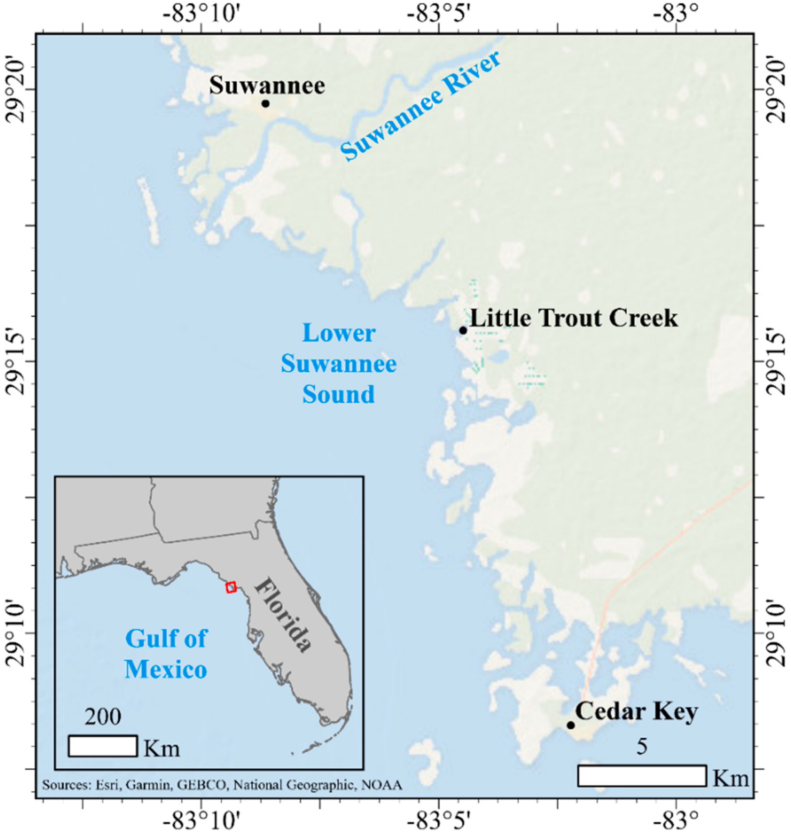
2.1. Study Site and UAS Survey

The study site is located at the mouth of Little Trout Creek (29°15′34.98″ N, 83°4′29.69″ W), within the Suwannee River estuary, on Florida’s Gulf of Mexico coast (Figure 1).
Little Trout Creek is a tidal creek with eastern oyster reef, salt marsh, and mudflat habitats present. This area is known to have sustained major changes in recent years and is of interest to local management agencies and researchers [25,26]. The Suwannee River estuary is within Florida’s Big Bend—the coastline from Crystal River to Apalachee Bay—where, as of 2011, there has been an estimated 66% net loss of the oyster reef area since 1982 [25]. There has also been evidence of increased erosion of islands in the region, coinciding with oyster reef decline and a decline in coastal forest coverage [26,27,28]. With about 100 km of federally protected coastline, the Suwannee River estuary is largely undeveloped, and 25% of the area’s economic activity is connected to natural resources [29,30]. Programs such as the Oyster Integrated Mapping and Monitoring Program (OIMMP) represent increasing efforts to map and monitor these resources [26].
A DJI Inspire 2 was used to collect georeferenced imagery on 8 December 2018 at the mouth of Little Trout Creek. The UAS was equipped with a Zenmuse X7 35 mm RGB sensor. A flying height of 60 m above ground level and image overlaps of 80% along-track and 75% across-track were set for the flight mission. Data collection was conducted to coincide with the low tide at 8:30 a.m. local time to maximize coverage of the emerged intertidal habitats. Four black-and-white checkered targets were deployed evenly across the scene. The location of the center of each target was recorded using real-time kinematic (RTK) positioning with a Trimble 5800 RTK system.

2.2. Imagery Processing

The survey produced 963 images and a ground sampling distance of 0.66 cm. Images were imported into the Pix4D Mapper v. 4.2.26, and ground control targets were located within the individual images and associated with coordinates recorded from RTK sampling to ensure the spatial quality of outputs [9,31]. Pix4D produced estimates of the position, angular orientation, and camera calibration parameters of images and generated an orthomosaic and a digital surface model (DSM) using structure from motion photogrammetry techniques (Figure 2). Ground control points were then digitized within the orthomosaic using ArcGIS Pro v 2.4 to calculate the spatial accuracy by comparing the coordinates to the known RTK observations [32].
The orthomosaic and DSM were then resampled to resolutions ranging from 3 to 31 cm by 2 cm increments. Resampling was conducted using the Resample tool with the nearest neighbor as the resampling method in ArcGIS Pro v 2.4, resulting in 15 datasets of different spatial resolutions. The lower limit of the range, 3 cm, was selected to be representative of high-resolution UAS imagery. The upper limit of 31 cm was selected to correspond with what can be acquired from other remote sensing sources (e.g., occupied aircraft imagery, satellite imagery). This method of varying the resolution scale of input variables (sometimes referred to as coarse-graining) has been used when studying marine environments, often within the context of habitat selection models [33,34,35,36], and was identified as the most appropriate method to use when wanting to characterize specific features or processes [17].

2.3. GEOBIA—Segmentation Optimization on Representative Subset Area

The analytical workflow is based on a geographic object-based image analysis (GEOBIA), which first segments the imagery into relatively homogeneous groups of pixels, forming meaningful objects, before classifying them [37,38,39]. Segmentation parameters are most often determined through trial and error, but here, we applied an optimization procedure to remove subjectivity from the analysis and facilitate end uses from non-experts. Figure 3 represents the workflow and the different tools used to accomplish each step.
First, a representative subset of the scene was taken from each mosaic to inform the optimization of the segmentation parameters (Figure 4). A subset was used for this procedure because it is computationally expensive. The optimization for each resolution was performed using the SegOptim package in R, providing a consistent and unbiased method for segmentation parameter selection [40]. The SegOptim package combines the optimization of segmentation parameters, image segmentation, and supervised classification in a single workflow. SegOptim relies on third-party software to produce segmentations. Here, the Orfeo ToolBox was selected, which provides open-source solutions for remote sensing analysis and contains applications that can be used within command lines [41]. The Orfeo ToolBox large-scale mean shift segmentation was selected to perform the segmentation, which has been shown to perform well in a variety of remote sensing applications and from medium to very high resolutions [42]. Three parameters drive the large-scale mean shift segmentation: spectral range radius (also referred to as range radius), spatial radius, and the minimum object size in pixels. Spatial radius refers to the radius of the neighborhood for averaging (higher spatial radius results in more smoothing). Spectral range radius refers to the degree of spectral variability, measured by the Euclidean distance (expressed in radiometry units) of the spectral signature that is allowed within an object (higher values preserve edges less than lower values) [43]. While higher values for spatial radius lead to more processing times, changing the spectral range radius does not affect the processing time [43]. Minimum size refers to the minimum allowable object size in pixels [43]. A range of appropriate values was set for each of the three parameters. Values ranging from 50 to 125 for the spectral range radius and 20 to 80 for the spatial radius were tested. The tested values for spectral and spatial radii remained constant for every tested resolution. The minimum object size values remained constant in terms of area, as the range in pixels was adjusted at every orthomosaic to allow for a minimum object size ranging from 7 to 10 m2. We selected this object size to correspond with the smallest habitat patch that we wanted to capture in the scene. As performed by Espriella et al. (2020), a 3 × 3 edge-detecting Laplacian filter was applied to each orthomosaic to serve as the input for the segmentation step, given its high performance in scenes where water is present. The “gaOptimizeSegmentationParams” command was used within the SegOptim package to test the quality of combinations within the defined parameter ranges. This function optimizes segmentation parameters using genetic algorithms [40]. The inputs of the genetic algorithm affect the computing time, as they direct functions, such as the number of iterations. These parameters were kept constant for all resolutions and can be found in Appendix A (Table A1).
To quantify the quality of the segmentation for each iteration, training data were provided in the form of rasters identifying samples for each of the four cover types (i.e., marsh, mud, oyster, and water) to conduct random forest classifications. Training areas were first manually delineated with polygons in ArcGIS Pro in a way to depict the geometry of each habitat patch (Figure 4). To be compatible with the SegOptim and Orfeo ToolBox workflow, the polygons were then exported as rasters using the Polygon to Raster tool in ArcGIS Pro. The training raster resolution for each optimization corresponded with the resolution of the orthomosaic being tested. These training areas were then used to identify the objects included in the random forest classifier. In order for an object from the segmentation to be included in the training dataset, 75% of its area must be within one of the delineated classes. The means and standard deviations of the three bands (red, green, blue) in the orthomosaic, calculated within segmented objects, were used to inform the classifier. A 10-fold cross-validation was used to evaluate the quality of each classification. The kappa coefficient of the classification was used as the metric to determine quality. The result of the optimization is the parameter values that produced the classification with the highest kappa value.

2.4. GEOBIA-Segmentation and Classification of the Entire Scene

Following the optimization, the parameter values from the output were applied to the entire scene. The implemented workflow follows the one introduced by Espriella et al. (2020). First, as with the subset (cf. Section 2.3), a 3 × 3 Laplacian filter of each respective resolution served as the layer for the large-scale mean shift segmentation. Following segmentation, the water objects were removed from the scene by setting their object ID to null within R. Given the homogeneity of the water, it is often segmented into just a few objects, and removing these objects limits confusion between water and adjacent classes.
After removing the water objects, the remaining segmented objects were ready to be classified. First, training areas were provided for the random forest classifier, as with the subset for the optimization step (Figure 5). As with the optimization, 75% of an object in the segmented layer must overlap with a training area in order to be used as training data for the classifier. The means and standard deviations of the red, green, and blue spectral layers and the DSM were used to inform the classifier.

2.5. Accuracy Assessment

Classification accuracy was quantified using a stratified random sampling scheme per class (i.e., marsh, mud, oyster, and water). Although the water class was not included within the random forest classifier, it was included in the accuracy assessment to quantify the accuracy of relying on the segmentation to delineate the water objects (cf. Section 2.4). The sample size for the number of points was determined using an equation based on a multinomial distribution with a 95% confidence level [44,45]. The sample size of 664 points was evenly distributed in ArcGIS Pro among the four classes to ensure equal representation. A confusion matrix was developed for each of the 15 resolutions tested. Producer-, user-, and overall accuracies, and a kappa coefficient, were calculated from each matrix. Producer’s accuracy measures how often real features are represented in the generated classification, while the user’s accuracy measures how often an object is erroneously included in a given class [46,47]. The Kappa coefficient quantifies accuracy as the actual agreement minus chance agreement [46]. In addition to these performance metrics, a mean decrease in Gini values from the random forest classifier was recorded to identify the most important inputs to the models. The mean decrease in Gini is the total decrease in node impurity for a predictor (when it forms a split in the forest), averaged across the trees [48,49]. The higher the value, the more influential the variable was in the classification.

2.6. Multiscale Analysis

To quantify agreement among the 15 classifications, each was resampled to 3 cm in ArcGIS using the Resample tool with the nearest neighbor as the resampling method. This allowed for the rasters to be stacked in R and the mode at each cell was recorded to determine the most agreed-upon class at that cell. A raster was generated from the mode values as well as a raster recording how many rasters within the stack of 15 predicted the mode class at a given cell. These representations allowed us to identify areas within the scene that may have caused significant confusion as evidenced by weak agreement between the classifications, as well as areas that performed well.
A classification that combined the most informative observation scales was also produced to quantify the accuracy of a multiscale classification. The resolutions that produced the best user accuracies for each of the four classes were combined in one raster stack. To stack the rasters, the orthomosaic and DSM were first resampled to the finest resolution of the four selected rasters using the same method as above. All four orthomosaics and DSMs were then stacked in R to generate one 16-band raster (3 spectral bands for each orthomosaic and 1 band for each DSM). The Laplacian filter of the finest resolution was used for segmentation using the parameters reported in the initial optimization procedure. The procedure then followed the steps from the individual resolution classification (cf. Section 2.4) and the accuracy assessment steps outlined above (cf. Section 2.5).

3. Results

3.1. Imagery Processing

From the digitized ground control points, a root mean square error of 2.1 cm in latitude and 1.6 cm in longitude was derived for the orthomosaic. Figure 6 shows the levels of detail allowed by the selected resolutions. The three-band orthomosaics ranged in size from 1.5 GB at 3 cm resolution to 15.5 MB at 31 cm. The DSMs range in size from 750 MB at 3 cm resolution to 7.7 MB at 31 cm.

3.2. Segmentation Optimization

Table 1 represents the spatial radius, spectral range radius, and minimum size parameter values that the SegOptim package reported as optimal for each resolution. The spatial radius was 58.5 on average across the resolutions, while the spectral range radius was 70.93 on average. The spatial radius was more variable than the spectral range radius, with standard deviations of 12.5 and 9.72, respectively. The average minimum object size was 7.57 m2 with a standard deviation of 0.47 m2.

3.3. Segmentation and Classification

Segmentations captured boundaries between habitats well, particularly between water and intertidal habitats (Figure A1). Given the relative homogeneity of the water surface, water was most often successfully grouped into a single object because adjacent objects did not exceed the spectral threshold parameter. However, up to three “water” objects were removed for some resolutions.
The average object for the mud class was the largest at 17.0 m2 (standard deviation = 1.8 m2). The average object in the oyster class was 16.3 m2 (standard deviation = 1.7 m2), and the marsh class had the smallest average object area of 15.7 m2 (standard deviation = 3.4 m2). Figure 7 displays the percent difference from the mean area over the 15 classifications per habitat type. The resolutions were largely consistent, with many displaying minimal differences from the mean value. However, some resolutions saw large variations. The 15 cm resolution produced the instance with the largest difference from the mean value with the marsh habitat representing 63% less area than the average marsh area among all classifications.

3.4. Accuracy Assessment

The classifications all performed well, with kappa coefficients ranging from 0.708 (29 cm resolution) to 0.764 (5 cm resolution). Overall accuracies ranged from 78% at 29 cm to 82% at 5 cm. The classifications with the highest and lowest performances are displayed in Figure 8.
Figure 9 represents the trend of kappa values over the range of resolutions. Performance was largely consistent over the span of the resolutions. The lowest-performing resolutions, 19 and 29 cm, struggled with differentiating mud from other habitat types, resulting in 56% and 60% producer accuracies, respectively. Most misclassifications within the mud class were with water for both the 19 cm and the 29 cm classifications. Very coarse resolutions performed similarly, and sometimes better than finer resolutions that took significantly more processing times.
While the kappa coefficient represents the classification’s performance across all classes, the user’s accuracy is of particular interest in this context, given the focus on monitoring and the value of the classifications to end users. The four cover types performed better in terms of user accuracies at different resolutions. Marsh and oyster performed better at coarser resolutions. The marsh habitat had a 96% user’s accuracy at 23 cm and the oyster habitat had an 84% user’s accuracy at 29 cm. Conversely, water and mud had the highest user accuracies at finer resolutions. Water performed best at 5 cm with a user’s accuracy of 86% and mud performed best at 3 cm with a user’s accuracy of 86%.

3.5. Variable Importance

The DSM mean was consistently the most influential metric included in the random forest classification, as measured by the mean decrease in Gini (Figure 10). The standard deviation of the DSM and standard deviation of the blue spectral band were the next most influential variables. While the standard deviation of the blue band and the standard deviation of the DSM produced similar mean decreases in Gini values for finer resolutions, beginning at the 21 cm resolution, the standard deviation of the DSM began indicating higher variable importance. This change may indicate that coarser resolutions are better able to characterize variations in habitat covers’ topography without the influence of noise, while the influence of spectral variation remains largely constant.

3.6. Mode of Classifications

The water class had the highest agreement among the classifications, averaging an agreement of 13.83 out of 15 rasters. Marsh had the next highest agreement at an average of 13.72, with oyster and mud displaying averages of 12.47 and 12.03, respectively. Areas of disagreement often corresponded with the edges of habitats, as evidenced by the outlines depicted in Figure 11. Areas of mud partially inundated with water (e.g., the southwest corner of the scene) also coincided with areas of disagreement between the classification rasters. Across the scene, 52% of the area had 100% agreement between the 15 rasters. When tested using the accuracy assessment points, the mode raster produced a kappa coefficient of 0.821 and overall accuracy of 87%. These high-performance metrics indicate that not only did classifications often agree, but also the agreed-upon class was frequently the correct class.

3.7. Multiscale Classification

The multiscale classification performed better than any individual classification in terms of the kappa coefficient and overall accuracy, producing results of 0.778 and 83%, respectively. However, there was a high level of omission for the mud class, resulting in a 57% producer’s accuracy. The mud class was most often misclassified as water. Despite the underperformance in terms of the producer’s accuracy, the user’s accuracy of 88% for mud was the highest among any of the classifications. The oyster class produced a user’s accuracy of 86%, which was also higher than any individual classification, while marsh and water had user accuracies of 89% and 75%, respectively. Table 2 shows the comparison of all classifications in terms of producer accuracies, user accuracies, overall accuracies, and kappa coefficients.
Variable importance was similar to that of the individual resolutions, with the DSM means as the most influential variable. However, 8 of 12 spectral standard deviations carried more importance than the DSM standard deviations. Figure A2 displays the mean decrease in Gini for the multiscale classification.

4. Discussion

4.1. Classification Performance

The GEOBIA classifications performed well at every resolution tested. The range of resolutions tested represents high-resolution UAS imagery (3 cm) up to what can be accessed via commercial satellite imagery (31 cm). Espriella et al. (2020) used GEOBIA to classify intertidal habitats with high accuracy. However, the workflow relied solely on the native resolution of the imagery, 6 mm. This ultra-high-resolution imagery resulted in lengthy processing times. The current study is unique in its exploration of different input resolutions in the GEOBIA workflow. While Espriella et al. (2020) used a multitude of layers, including spectral indices and geometric properties to develop a classification workflow, this study relies only on the orthomosaic and DSM to further encourage straightforward and consistent monitoring.
The high performance of the classification workflow over the range of resolutions indicates that targeting excessively fine resolutions on the scale of millimeters or 1 cm may not be necessary for intertidal habitat mapping purposes along Florida’s Big Bend coastline. Coarser resolutions correspond with higher flying heights for UASs, meaning more area can be covered in a single mission. The ability to yield greater coverage without sacrificing classification accuracy has significant implications for monitoring agencies that have limited resources. The 19 and 29 cm resolutions performed more modestly than the other resolutions, but still produced high-performance metrics for habitat mapping applications. Despite their lower accuracies, kappa coefficients of 0.713 (19 cm) and 0.708 (29 cm) are very promising metrics. Kappa values between 0.6 and 0.8 are considered to have a ‘substantial’ agreement, which is the case for all tested resolutions [50]. Additionally, there was substantial agreement between the classifications at multiple scales (Figure 11). This agreement provides further evidence that for habitat mapping, very fine resolutions may not be necessary for this environment. Despite the high performances of the classifications at resolutions that coincide with occupied aerial or satellite imagery, it is important to note that such imagery is rarely captured at the ideal conditions (e.g., lowest tides and adequate scene illumination) allowable by the flexibility of UAS surveys.
To increase the accuracy of the classifications, steps should be explored to better differentiate mud, as it was the class that performed the worst in terms of producer’s accuracy in 12 of the 15 resolutions tested. The mud class was most often confused with water, followed by the oyster. From a classification perspective, mud has the disadvantage of having qualities that may be consistent with water when examining the DSM (i.e., relatively low elevation and homogenous surface), while having qualities that may be consistent with oysters in terms of the spectral response characterized in the orthomosaic.
Although classification accuracy is useful to quantify the reliability of a habitat map, there is often limited understanding of the location of errors or areas of low accuracy [51]. As evidenced by Figure 11, classification errors are frequently related to habitat patch boundaries and transitionary zones [51,52,53]. The map displaying the percent agreement highlights how the edges of habitats coincided with lower levels of agreement among classifications. The southwest corner of the study area was also a challenging area. This area was primarily mud that was partially inundated with water at the time of the survey, explaining why there was disagreement among the classifications at the different resolutions. Figure 7 also provides insight into challenges with boundaries. While most classifications produced similar habitat areas, the 15 cm resolution produced significantly less marsh habitat, as the edges of the habitat were often segmented into water objects. The inclusion of structural features beyond the DSM has the potential to improve the segmentation in these areas. Additionally, classifications based on fuzzy logic principles would potentially help improve results in these challenging environments as they can better represent natural transitional areas between habitat types; they do not impose discrete boundaries between adjacent habitat types [54]. Fuzzy logic and other soft classification principles also allow objects to belong to more than one class. This could improve areas such as mud inundated with water and fringing oysters that integrate with the salt marsh habitat.
While the classifications performed well at each resolution, there were notable findings regarding which scale best characterized each cover type. Water and mud performed best in terms of user accuracies at finer scales of 5 and 3 cm, respectively. Conversely, marsh and oyster habitats produced the highest user accuracies at coarser resolutions of 23 and 29 cm, respectively. Selecting a proper observational scale is an ongoing area of research as no one scale is appropriate for the study of all ecological processes [19,55,56,57]. Multiscale workflows can help address the limitations of single-scale workflows by highlighting those that are most informative, a consideration that is as important as variable selection [19].
Lecours and Espriella (2020) suggest that multiscale roughness metrics can help delineate intertidal habitats [57]. The study finds that mudflats present a comparatively lower magnitude of roughness, with the highest roughness values captured at coarse scales. Conversely, the marsh habitat displayed the highest magnitude of roughness among the habitats and did so at a fine scale. Oyster reefs displayed an intermediate magnitude of roughness at an intermediate scale when compared to mudflat and marsh habitats. These findings within the context of the current study highlight the significance of variable importance, relative to the scale (Figure A2). The mean of the DSM as the most influential parameter across the tested resolutions is logical, given the varying elevations across the cover types. The standard deviation of the DSM and the standard deviation of the blue spectral band were the next most influential parameters, following the DSM mean. The standard deviation of the DSM exhibited a higher level of importance at coarser scales when compared to the blue spectral band standard deviation. The standard deviation of the DSM highlights topographic heterogeneity, and with the assumption that marsh and oyster habitats are more structurally complex than mud and water, should contribute to the classification accordingly. However, it is notable that in terms of classification accuracy, the habitats performed counter to these assumptions. Marsh and oyster habitats had the highest performances in terms of user accuracies at coarser scales, while mud and water had their highest performance at finer scales. Despite these differences, it is also important to consider that classifications performed well across the resolutions (e.g., the marsh class displayed its highest user accuracy of 96% at 23 cm, but also had a user accuracy of 90% at 3 cm). These differences again highlight that scale selection should be context-dependent.
The multiscale classification conducted further demonstrates the relevancy of using multiscale workflows. The multiscale classification performed better than any individual resolution in terms of the kappa coefficient and provided further insight into which variables are most important to consider (Figure A2). As with the single-scale classifications, the DSM means were the most influential. However, unlike the single-scale classifications, the standard deviations of the spectral bands, highlighting spectral heterogeneity, were often more influential than the DSM standard deviations (Figure A2). Additionally, the spectral variation was most influential at finer scales, suggesting the signatures of the habitat types may be lost at coarser scales. The classification generated by the mode of each individual resolution produced a very high kappa coefficient of 0.821, demonstrating the utility of quantifying a classification agreement (Figure 11). However, this method was used primarily to understand areas of uncertainty and would be computationally intensive to rely on for consistent monitoring.

4.2. Considerations, Challenges, and Future Directions

While the Orfeo ToolBox large-scale mean shift algorithm produced quality segmentations, there were initial challenges with arriving at an appropriate segmentation for the scene. The segmentation developed artifacts across flight paths, likely caused by a slight variation in atmospheric conditions and tide levels that generated artificial changes in spectral response. As a result, objects would display boundaries in a north–south orientation, given the east–west flight pattern of the UAS. The SegOptim package supports multiple segmentation algorithms from third-party software. The RSGISLib Shepherd’s k-means segmentation was tested before the Orfeo ToolBox large-scale mean shift segmentation. However, after exploring the data and segmentations, there was significant difficulty in reconciling the flight path artifacts. The large-scale mean shift better handled any artifacts introduced by flight paths. In future studies, this can be partially addressed by including a light sensor on the UAS that normalizes spectral responses by measuring incoming light. Another difficulty was posed during the testing of classifications in the optimization step. In order for the optimization to run completely, the validation must produce a specified minimum number of train cases and test cases; regarding the optimizations conducted for this study, five of each were required (Table A1). For this dataset, this meant finding a middle ground that generated representative objects that did not compromise their shapes or sizes, while maintaining enough objects to meet the testing parameters. For example, setting the spectral range radius too high would result in all water objects in the subset for optimization being merged. As a result, there would not be sufficient objects to run validation steps. Another processing consideration was the inclusion of the DSM. The DSM was not included in the optimization procedure, as the optimization is very computationally intensive. Additionally, non-expert end users may not have the ability or resources to develop quality digital surface models. Therefore, by excluding it from the optimization, it ensures end users can rely on the optimized segmentation parameters when only using an orthomosaic (or potentially a single) image in the case of an occupied aircraft or satellite imagery.
Despite the near-equal performances across the different resolutions for classification, results for studies that target other objectives, such as analyzing habitat geometries, could prove different as the resolution changes. For example, should one be interested in calculating the perimeter of oyster reefs for spatial analysis, the resolution is an important consideration. To illustrate this fact, a classified oyster reef at the 5 cm resolution had an area of 2106 m2 and a perimeter of 1879 m, while the same reef had an area of 2005 m2 and a perimeter of 949 m at the 31 cm resolution. While the area was largely preserved, seeing only a 4.9% difference between the resolutions, the perimeters represent a 65.8% difference. This difference highlights how researchers must consider the scale-dependency of metrics, as the area proved to be less scale-dependent than the perimeter. Ultimately, it is essential to consider objectives when selecting an appropriate target resolution [16]. No one scale of observation is suitable for all objectives, and when using imagery to study ecological processes, the scale should be considered within the context of the biological and environmental processes being studied [16,19,58,59].
While this study used only three spectral bands, given the accessibility of RGB sensors, spectral resolution is another important consideration in habitat mapping workflows. For example, Chand and Bollard (2021) suggest that spectral resolution is more critical to classify oyster reefs than spatial resolution, as an RGB dataset with a higher spatial resolution did not perform as well as a coarser dataset that included red-edge and near-infrared bands [60]. The inclusion of a near infrared band has the potential to better differentiate water and mud, where most misclassifications occurred, given its ability to differentiate water and non-water bodies [61]. Optimizing spectral resolution along with spatial resolution will further improve habitat classifications and our understanding of what metrics to target in data collection.
The GEOBIA workflow detailed in this study was conducted within R using open-source solutions. An example of the workflow is made available in the Supplementary Materials. This study was able to achieve a similar level of accuracy as the one by Espriella et al. (2020), which relied on proprietary software. This accessibility allows for consistent, holistic monitoring of intertidal habitats along Florida’s Gulf of Mexico coastline. Future surveys can use the results of this study to decide what is an appropriate resolution, or resolutions, for the monitoring objectives. This workflow streamlines data collection and processing for future studies in the intertidal. While altitude (and indirectly, resolution) has the strongest effect on flight time, other flight parameters, such as image overlaps, can also be studied to quantify trade-offs and further streamline the process [13].

5. Conclusions

Florida’s intertidal habitats along the Gulf of Mexico coast are dynamic ecosystems experiencing significant changes. Generating reliable methods to monitor these resources allows management to appropriately respond to their potential deterioration. Remote sensing platforms such as UASs provide resources to conduct consistent temporal monitoring. Here, classifications were conducted using GEOBIA to determine how scale affects the accuracy of habitat maps produced at different resolutions. In general, results showed that classification accuracy did not change dramatically when coarsening data resolution, which has direct implications for data collection and processing. Results also (1) confirmed that one single scale is not optimal for the study of all habitat types; (2) showed how promising the implementation of multiscale analysis is for coastal habitat classification; and (3) highlighted that fuzzy classifications should be explored to capture the areas of transition among habitat types, which were often the sources of misclassification. Coupling information obtained from sensors with a repeatable workflow that is freely available provides managers with the necessary tools to conduct consistent monitoring and identifies scales and variables of interest for three intertidal habitat types. The inclusion of GEOBIA within the workflow also creates many other possibilities, such as quantifying spatial relationships among habitats or tracking geometries, as commonly performed in seascape ecology. Habitat maps are valuable tools for quantifying change; this study contributes to the present knowledge gaps regarding best practices to collect and process high-quality data.

Supplementary Materials

The following supporting information can be downloaded at: https://www.mdpi.com/article/10.3390/drones6060140/s1, R code example.

Author Contributions

Conceptualization, M.C.E. and V.L.; methodology, M.C.E.; software, M.C.E.; validation, M.C.E.; formal analysis, M.C.E.; investigation, M.C.E.; resources, M.C.E. and V.L.; data curation, M.C.E.; writing—original draft preparation, M.C.E.; writing—review and editing, M.C.E. and V.L.; visualization, M.C.E.; supervision, V.L.; project administration, V.L.; funding acquisition, V.L. All authors have read and agreed to the published version of the manuscript.

Funding

This work was supported by the USDA National Institute of Food and Agriculture (Hatch project FLA-FOR-005981; multiscale analysis of oyster resources using geomorphometry and remote sensing technologies), by funds allocated to V.L. by the University of Florida Senior Vice President for Agriculture and Natural Resources, and by an Early-Career Research Fellowship to V.L. from the Gulf Research Program of the National Academies of Sciences, Engineering, and Medicine.

Informed Consent Statement

Not applicable.

Data Availability Statement

Data can be made available upon reasonable request.

Acknowledgments

Thanks are due to Peter Frederick for providing the imagery and Steve Beck, Sean Denney, Lindsey Garner, and Andrew Ortega who led the imagery and RTK data collection. Additional thanks go out to João Gonçalves for providing support with the SegOptim package.

Conflicts of Interest

The authors declare no conflict of interest.

Appendix A

Table A1. Parameters used in the SegOptim optimization step.
ParameterValue Used
Training threshold0.75
Balance method“ubOver” (over-sampling)
Evaluation metric“Kappa” (kappa coefficient)
Evaluation method“10FCV” (10-fold cross-validation)
Min train cases20
Min cases by class train5
Min cases by class test5
Population size20
Probability of crossover0.8
Probability of mutation0.2
Max number of iterations5
Run20
Keep bestTRUE
Figure A1. The 5 cm segmentation with (left) and without (right) the water object. In the case of the 5 cm resolution, water was segmented into a single object. Given the spectral homogeneity of the water, multiple objects were merged into one because adjacent objects did not exceed the spectral threshold outlined by the spectral range radius parameter.
Drones 06 00140 g0a1
Figure A2. The mean decrease in Gini for each metric included in the multiscale classification.
Drones 06 00140 g0a2

References

  1. Wiens, J.A. Landscape Mosaics and Ecological Theory. In Mosaic Landscapes and Ecological Processes; Hansson, L., Fahrig, L., Merriam, G., Eds.; Springer: Dordrecht, The Netherlands, 1995; pp. 1–26. [Google Scholar]
  2. Wedding, L.M.; Lepczyk, C.A.; Pittman, S.J.; Friedlander, A.M.; Jorgensen, S. Quantifying Seascape Structure: Extending Terrestrial Spatial Pattern Metrics to the Marine Realm. Mar. Ecol. Prog. Ser. 2011, 427, 219–232. [Google Scholar] [CrossRef]
  3. Olds, A.D.; Nagelkerken, I.; Huijbers, C.M.; Gilby, B.L.; Pittman, S.J.; Schlacher, T.A. Connectivity in Coastal Seascapes. In Seascape Ecology, 1st ed.; Pittman, S.J., Ed.; John Wiley & Sons Ltd.: Hoboken, NJ, USA, 2018; pp. 261–364. [Google Scholar]
  4. Pittman, S.J. Introducing Seascape Ecology. In Seascape Ecology, 1st ed.; Pittman, S.J., Ed.; John Wiley & Sons Ltd.: Hoboken, NJ, USA, 2018; pp. 1–25. [Google Scholar]
  5. Meyer, D.L.; Townsend, E.C.; Thayer, G.W. Stabilization and Erosion Control Value of Oyster Cultch for Intertidal Marsh. Restor. Ecol. 1997, 5, 93–99. [Google Scholar] [CrossRef]
  6. Grabowski, J.H.; Hughes, A.R.; Kimbro, D.L.; Dolan, M.A. How Habitat Setting Influences Restored Oyster Reef Communities. Ecology 2005, 86, 1926–1935. [Google Scholar] [CrossRef]
  7. Hosack, G.R.; Dumbauld, B.R.; Ruesink, J.L.; Armstrong, D.A. Habitat Associations of Estuarine Species: Comparisons of Intertidal Mudflat, Seagrass (Zostera Marina), and Oyster (Crassostrea Gigas) Habitats. Estuaries Coasts 2006, 29, 1150–1160. [Google Scholar] [CrossRef]
  8. Smyth, A.R.; Piehler, M.F.; Grabowski, J.H. Habitat Context Influences Nitrogen Removal by Restored Oyster Reefs. J. Appl. Ecol. 2015, 52, 716–725. [Google Scholar] [CrossRef]
  9. Windle, A.E.; Poulin, S.K.; Johnston, D.W.; Ridge, J.T. Rapid and Accurate Monitoring of Intertidal Oyster Reef Habitat Using Unoccupied Aircraft Systems and Structure from Motion. Remote Sens. 2019, 11, 2394. [Google Scholar] [CrossRef]
  10. Espriella, M.C.; Lecours, V.; Frederick, P.C.; Camp, E.V.; Wilkinson, B. Quantifying Intertidal Habitat Relative Coverage in a Florida Estuary Using UAS Imagery and GEOBIA. Remote Sens. 2020, 12, 677. [Google Scholar] [CrossRef]
  11. Ridge, J.T.; Gray, P.C.; Windle, A.E.; Johnston, D.W. Deep Learning for Coastal Resource Conservation: Automating Detection of Shellfish Reefs. Remote Sens. Ecol. Conserv. 2020, 6, 431–440. [Google Scholar] [CrossRef]
  12. Fraser, B.T.; Congalton, R.G. Issues in Unmanned Aerial Systems (UAS) Data Collection of Complex Forest Environments. Remote Sens. 2018, 10, 908. [Google Scholar] [CrossRef]
  13. Seifert, E.; Seifert, S.; Vogt, H.; Drew, D.; van Aardt, J.; Kunneke, A.; Seifert, T. Influence of Drone Altitude, Image Overlap, and Optical Sensor Resolution on Multi-View Reconstruction of Forest Images. Remote Sens. 2019, 11, 1252. [Google Scholar] [CrossRef]
  14. Whitehead, K.; Hugenholtz, C.H. Remote Sensing of the Environment with Small Unmanned Aircraft Systems (UASs), Part 1: A Review of Progress and Challenges. J. Unmanned Veh. System 2014, 2, 69–85. [Google Scholar] [CrossRef]
  15. Torres-Sánchez, J.; López-Granados, F.; Borra-Serrano, I.; Peña, J.M. Assessing UAV-Collected Image Overlap Influence on Computation Time and Digital Surface Model Accuracy in Olive Orchards. Precis. Agric. 2018, 19, 115–133. [Google Scholar] [CrossRef]
  16. Lecours, V.; Devillers, R.; Schneider, D.; Lucieer, V.; Brown, C.; Edinger, E. Spatial Scale and Geographic Context in Benthic Habitat Mapping: Review and Future Directions. Mar. Ecol. Prog. Ser. 2015, 535, 259–284. [Google Scholar] [CrossRef]
  17. Misiuk, B.; Lecours, V.; Dolan, M.F.J.; Robert, K. Evaluating the Suitability of Multi-Scale Terrain Attribute Calculation Approaches for Seabed Mapping Applications. Mar. Geod. 2021, 44, 327–385. [Google Scholar] [CrossRef]
  18. Miyamoto, M.; Kiyota, M.; Murase, H.; Nakamura, T.; Hayashibara, T. Effects of Bathymetric Grid-Cell Sizes on Habitat Suitability Analysis of Cold-Water Gorgonian Corals on Seamounts. Mar. Geod. 2017, 40, 205–223. [Google Scholar] [CrossRef]
  19. Misiuk, B.; Lecours, V.; Bell, T. A Multiscale Approach to Mapping Seabed Sediments. PLoS ONE 2018, 13, e0193647. [Google Scholar]
  20. Florinsky, I.V.; Kuryakova, G.A. Determination of Grid Size for Digital Terrain Modelling in Landscape Investigations—Exemplified by Soil Moisture Distribution at a Micro-Scale. Int. J. Geogr. Inf. Sci. 2000, 14, 815–832. [Google Scholar] [CrossRef]
  21. Gottschalk, T.K.; Aue, B.; Hotes, S.; Ekschmitt, K. Influence of Grain Size on Species–Habitat Models. Ecol. Model. 2011, 222, 3403–3412. [Google Scholar] [CrossRef]
  22. Dolan, M.F.J.; Van Lancker, V.; Guinan, J.; Al-Hamdani, Z.; Leth, J.; Thorsnes, T. Terrain Characterization from Bathymetry Data at Various Resolutions in European Waters—Experiences and Recommendations; Geological Survey of Norway Report No. 2012.045; Geological Survey of Norway: Trondheim, Norway, 2012.
  23. Blanchet, H.; Gouillieux, B.; Alizier, S.; Amouroux, J.-M.; Bachelet, G.; Barillé, A.-L.; Dauvin, J.-C.; de Montaudouin, X.; Derolez, V.; Desroy, N.; et al. Multiscale Patterns in the Diversity and Organization of Benthic Intertidal Fauna among French Atlantic Estuaries. J. Sea Res. 2014, 90, 95–110. [Google Scholar] [CrossRef]
  24. Azhar, M.; Schenone, S.; Anderson, A.; Gee, T.; Cooper, J.; van der Mark, W.; Hillman, J.R.; Yang, K.; Thrush, S.F.; Delmas, P. A Framework for Multiscale Intertidal Sandflat Mapping: A Case Study in the Whangateau Estuary. ISPRS J. Photogramm. Remote Sens. 2020, 169, 242–252. [Google Scholar] [CrossRef]
  25. Seavey, J.R.; Pine III, W.E.; Frederick, P.; Sturmer, L.; Berrigan, M. Decadal Changes in Oyster Reefs in the Big Bend of Florida’s Gulf Coast. Ecosphere 2011, 2, 1–14. [Google Scholar] [CrossRef]
  26. Radabaugh, K.R.; Geiger, S.P.; Moyer, P.P. Oyster Integrated Mapping and Monitoring Program Report for the State of Florida; FWRI Technical Report No. 22; Fish and Wildlife Research Institute, Florida Fish and Wildlife Conservation Commission: St. Petersburg, FL, USA, 2019. [Google Scholar]
  27. McCarthy, M.J.; Dimmitt, B.; Muller-Karger, F.E. Rapid Coastal Forest Decline in Florida’s Big Bend. Remote Sens. 2018, 10, 1721. [Google Scholar] [CrossRef]
  28. Vitale, N.; Brush, J.; Powell, A. Loss of Coastal Islands Along Florida’s Big Bend Region: Implications for Breeding American Oystercatchers. Estuaries Coasts 2021, 44, 1173–1182. [Google Scholar] [CrossRef]
  29. Main, M.B.; Allen, G.M. Florida’s Environment: North Central Region; Wildlife Ecology and Conservation Department, Florida Cooperative Extension Service, Institute of Food and Agricultural Sciences, University of Florida: Gainesville, FL, USA, 2007. [Google Scholar]
  30. Moore, J.F.; Pine, W.E., III; Frederick, P.C.; Beck, S.; Moreno, M.; Dodrill, M.J.; Boone, M.; Sturmer, L.; Yurek, S. Trends in Oyster Populations in the Northeastern Gulf of Mexico: An Assessment of River Discharge and Fishing Effects over Time and Space. Mar. Coast. Fish. 2020, 12, 191–204. [Google Scholar] [CrossRef]
  31. Pix4D Mapper [Computer Software]. Available online: https://www.pix4d.com/product/pix4dmapperphotogrammetry-software (accessed on 1 March 2022).
  32. ESRI ArcGIS Pro v 2.4 [Computer Software]. Available online: https://pro.arcgis.com/es/pro-app (accessed on 1 March 2022).
  33. Alvarez-Berastegui, D.; Ciannelli, L.; Aparicio-Gonzalez, A.; Reglero, P.; Hidalgo, M.; López-Jurado, J.L.; Tintoré, J.; Alemany, F. Spatial Scale, Means and Gradients of Hydrographic Variables Define Pelagic Seascapes of Bluefin and Bullet Tuna Spawning Distribution. PLoS ONE 2014, 9, e109338. [Google Scholar] [CrossRef]
  34. Scales, K.L.; Hazen, E.L.; Jacox, M.G.; Edwards, C.A.; Boustany, A.M.; Oliver, M.J.; Bograd, S.J. Scale of Inference: On the Sensitivity of Habitat Models for Wide-Ranging Marine Predators to the Resolution of Environmental Data. Ecography 2017, 40, 210–220. [Google Scholar] [CrossRef]
  35. Pittman, S.J.; Brown, K.A. Multi-Scale Approach for Predicting Fish Species Distributions across Coral Reef Seascapes. PLoS ONE 2011, 6, e20583. [Google Scholar] [CrossRef]
  36. Schneider, D.C. Scale and Scaling in Seascape Ecology. In Seascape Ecology, 1st ed.; Pittman, S.J., Ed.; John Wiley & Sons Ltd.: Hoboken, NJ, USA, 2018; pp. 89–117. [Google Scholar]
  37. Gibbes, C.; Adhikari, S.; Rostant, L.; Southworth, J.; Qiu, Y. Application of Object Based Classification and High Resolution Satellite Imagery for Savanna Ecosystem Analysis. Remote Sens. 2010, 2, 2748–2772. [Google Scholar] [CrossRef]
  38. Blaschke, T. Object Based Image Analysis for Remote Sensing. ISPRS J. Photogramm. Remote Sens. 2010, 65, 2–16. [Google Scholar] [CrossRef]
  39. Diesing, M.; Green, S.L.; Stephens, D.; Lark, R.M.; Stewart, H.A.; Dove, D. Mapping Seabed Sediments: Comparison of Manual, Geostatistical, Object-Based Image Analysis and Machine Learning Approaches. Cont. Shelf Res. 2014, 84, 107–119. [Google Scholar] [CrossRef]
  40. Gonçalves, J.; Pôças, I.; Marcos, B.; Mücher, C.A.; Honrado, J.P. SegOptim—A New R Package for Optimizing Object-Based Image Analyses of High-Spatial Resolution Remotely-Sensed Data. Int. J. Appl. Earth Obs. Geoinf. 2019, 76, 218–230. [Google Scholar] [CrossRef]
  41. Grizonnet, M.; Michel, J.; Poughon, V.; Inglada, J.; Savinaud, M.; Cresson, R. Orfeo ToolBox: Open Source Processing of Remote Sensing Images. Open Geospat. Data Softw. Stand. 2017, 2, 15. [Google Scholar] [CrossRef]
  42. Michel, J.; Youssefi, D.; Grizonnet, M. Stable Mean-Shift Algorithm and Its Application to the Segmentation of Arbitrarily Large Remote Sensing Images. IEEE Trans. Geosci. Remote Sens. 2015, 53, 952–964. [Google Scholar] [CrossRef]
  43. OTB Development Team. OTB CookBook Documentation; CNES: Paris, France, 2018.
  44. Jensen, J.R. Introductory Digital Image Processing: A Remote Sensing Perspective, 3rd ed.; Pearson Education: Upper Saddle River, NJ, USA, 2005. [Google Scholar]
  45. Congalton, R.G. A review of assessing the accuracy of classifications in remotely sensed data. Remote Sens. Environ. 1991, 37, 35–46. [Google Scholar] [CrossRef]
  46. Fung, T.; LeDrew, E. The determination of optimal threshold levels for change detection using various accuracy indices. Photogramm. Eng. Remote Sens. 1988, 54, 1449–1454. [Google Scholar]
  47. Story, M.; Congalton, R.G. Accuracy assessment: A user’s perspective. Photogramm. Eng. Remote Sens. 1986, 52, 397–399. [Google Scholar]
  48. Luz Calle, M.; Urrea, V. Letter to the Editor: Stability of Random Forest Importance Measures. Brief. Bioinform. 2011, 12, 86–89. [Google Scholar] [CrossRef]
  49. Han, H.; Guo, X.; Yu, H. Variable Selection Using Mean Decrease Accuracy and Mean Decrease Gini Based on Random Forest. In Proceedings of the 2016 7th IEEE International Conference on Software Engineering and Service Science (ICSESS), Beijing, China, 26–28 August 2016; pp. 219–224. [Google Scholar]
  50. Landis, J.R.; Kock, G.G. The measurement of observer agreement for categorical data. Biometrics 1977, 33, 159–174. [Google Scholar] [CrossRef] [PubMed]
  51. Langford, W.T.; Gergel, S.E.; Dietterich, T.G.; Cohen, W. Map Misclassification Can Cause Large Errors in Landscape Pattern Indices: Examples from Habitat Fragmentation. Ecosystems 2006, 9, 474–488. [Google Scholar] [CrossRef]
  52. Edwards, G.; Lowell, K.E. Modeling Uncertainty in Photointerpreted Boundaries. Photogramm. Eng. Remote Sens. 1996, 15, 377–391. [Google Scholar]
  53. Plourde, L.; Congalton, R. Sampling Method and Sample Placement: How Do They Affect the Accuracy of Remotely Sensed Maps? Photogramm. Eng. Remote Sens. 2003, 69, 289–297. [Google Scholar] [CrossRef]
  54. Fiorentino, D.; Lecours, V.; Brey, T. On the Art of Classification in Spatial Ecology: Fuzziness as an Alternative for Mapping Uncertainty. Front. Ecol. Evol. 2018, 6, 231. [Google Scholar] [CrossRef]
  55. Wiens, J.A. Spatial Scaling in Ecology. Funct. Ecol. 1989, 3, 385–397. [Google Scholar] [CrossRef]
  56. Willis, K.J.; Whittaker, R.J. Species Diversity—Scale Matters. Science 2002, 295, 1245–1248. [Google Scholar] [CrossRef] [PubMed]
  57. Lecours, V.; Espriella, M. Can Multiscale Roughness Help Computer-Assisted Identification of Coastal Habitats in Florida? In Proceedings of the Geomorphometry 2020 Conference, Perugia, Italy, 22–26 June 2020; IRPI CNR: Perugia, Italy, 2020. [Google Scholar]
  58. Goodchild, M.F. Scale in GIS: An Overview. Geomorphology 2011, 130, 5–9. [Google Scholar] [CrossRef]
  59. Bradter, U.; Kunin, W.E.; Altringham, J.D.; Thom, T.J.; Benton, T.G. Identifying Appropriate Spatial Scales of Predictors in Species Distribution Models with the Random Forest Algorithm. Methods Ecol. Evol. 2013, 4, 167–174. [Google Scholar] [CrossRef]
  60. Chand, S.; Bollard, B. Low Altitude Spatial Assessment and Monitoring of Intertidal Seagrass Meadows beyond the Visible Spectrum Using a Remotely Piloted Aircraft System. Estuar. Coast. Shelf Sci. 2021, 255, 107299. [Google Scholar] [CrossRef]
  61. Mondejar, J.P.; Tongco, A.F. Near Infrared Band of Landsat 8 as Water Index: A Case Study around Cordova and Lapu-Lapu City, Cebu, Philippines. Sustain Environ. Res. 2019, 29, 16. [Google Scholar] [CrossRef]
Figure 1. Study site for the UAS survey. The mouth of Little Trout Creek is located within the larger tidal environment of the Suwannee Sound, fed by the Suwannee River in the Gulf of Mexico.
Drones 06 00140 g001
Figure 2. Orthomosaic and DSM at the native imagery resolution of 0.66 cm.
Drones 06 00140 g002
Figure 3. Diagram detailing the workflow from data acquisition to habitat classification.
Drones 06 00140 g003
Figure 4. Training subset and delineated training areas for segmentation optimization.
Drones 06 00140 g004
Figure 5. Delineated training areas for the classification of the entire scene.
Drones 06 00140 g005
Figure 6. Area of about 10 × 10 m with marsh, oyster, mud, and water at varying resolutions. A checkered ground control target is visible in some of the resolutions. The difference in details for each resolution highlights how even an expert/manual delineation of these habitats by photointerpretation would lead to different results.
Drones 06 00140 g006
Figure 7. The percent difference from the mean area across the 15 classifications for each class at the respective resolution. This visualization allows for initial observations about what classes are being confused for each other (e.g., when there is a large difference in the mud class, there is also often a large difference in the water class that offsets).
Drones 06 00140 g007
Figure 8. Classification corresponding with the highest kappa coefficient at 5 cm (left) compared to the 29 cm resolution (right), which had the lowest kappa coefficient. The comparison allows visualizing areas within the scene that pose challenges, such as the southwest corner where mud is mistaken for water in the 29 cm classification.
Drones 06 00140 g008
Figure 9. Change in kappa coefficient as a function of input resolution.
Drones 06 00140 g009
Figure 10. Boxplots representing the mean decrease in Gini for each input variable over the range of resolutions. Black dots represent outliers.
Drones 06 00140 g010
Figure 11. The class most often represented in each raster cell (left) and how often that class was represented out of the 15 classifications (right).
Drones 06 00140 g011
Table 1. Results for each parameter at the respective resolution.
ResolutionSpectral RadiusSpatial RadiusMin Size (Pixels)Min Size (m2)
3 cm565682867.46
5 cm636129327.33
7 cm657116267.97
9 cm71399317.54
11 cm62707408.96
13 cm69554557.69
15 cm63453297.40
17 cm67552617.54
19 cm86592077.47
21 cm76771617.10
23 cm86731337.04
25 cm74391137.06
27 cm66601077.80
29 cm8972927.73
31 cm7145777.40
Table 2. Performance metrics for each of the individual scale classifications, and the two multiscale methods. PA refers to producer’s accuracy and UA refers to user’s accuracy.
MarshMudOysterWater
PAUAPAUAPAUAPAUAOverallKappa
3 cm92%90%49%86%87%74%96%75%80%0.736
5 cm92%86%73%77%78%80%88%86%82%0.764
7 cm88%89%73%71%72%84%87%76%79%0.727
9 cm91%92%69%83%75%77%90%74%81%0.743
11 cm93%92%80%74%75%78%77%83%81%0.749
13 cm89%93%72%74%74%76%83%77%79%0.723
15 cm88%95%74%74%81%71%77%82%80%0.728
17 cm91%89%78%75%73%84%86%80%82%0.757
19 cm85%95%56%80%80%76%93%69%78%0.713
21 cm93%91%72%78%78%82%87%78%82%0.759
23 cm88%96%67%74%78%81%87%72%80%0.732
25 cm88%90%72%78%78%81%89%77%81%0.751
27 cm95%89%67%83%82%71%82%83%81%0.745
29 cm85%90%60%82%73%84%97%64%78%0.708
31 cm87%91%75%79%79%83%89%77%82%0.763
Mode95%93%76%87%86%84%91%83%87%0.821
Multiscale92%89%58%88%86%86%96%75%83%0.778
Publisher’s Note: MDPI stays neutral with regard to jurisdictional claims in published maps and institutional affiliations.

