Aircraft Carrier Pose Tracking Based on Adaptive Region in Visual Landing

Abstract

Due to its structural simplicity and its strong anti-electromagnetic ability, landing guidance based on airborne monocular vision has gained more and more attention. Monocular 6D pose tracking of the aircraft carrier is one of the key technologies in visual landing guidance. However, owing to the large range span in the process of carrier landing, the scale of the carrier target in the image variates greatly. There is still a lack of robust monocular pose tracking methods suitable for this scenario. To tackle this problem, a new aircraft carrier pose tracking algorithm based on scale-adaptive local region is proposed in this paper. Firstly, the projected contour of the carrier target is uniformly sampled to establish local circular regions. Then, the local area radius is adjusted according to the pixel scale of the projected contour to build the optimal segmentation energy function. Finally, the 6D pose tracking of the carrier target is realized by iterative optimization. Experimental results on both synthetic and real image sequences show that the proposed method achieves robust and efficient 6D pose tracking of the carrier target under the condition of large distance span, which meets the application requirements of carrier landing guidance.

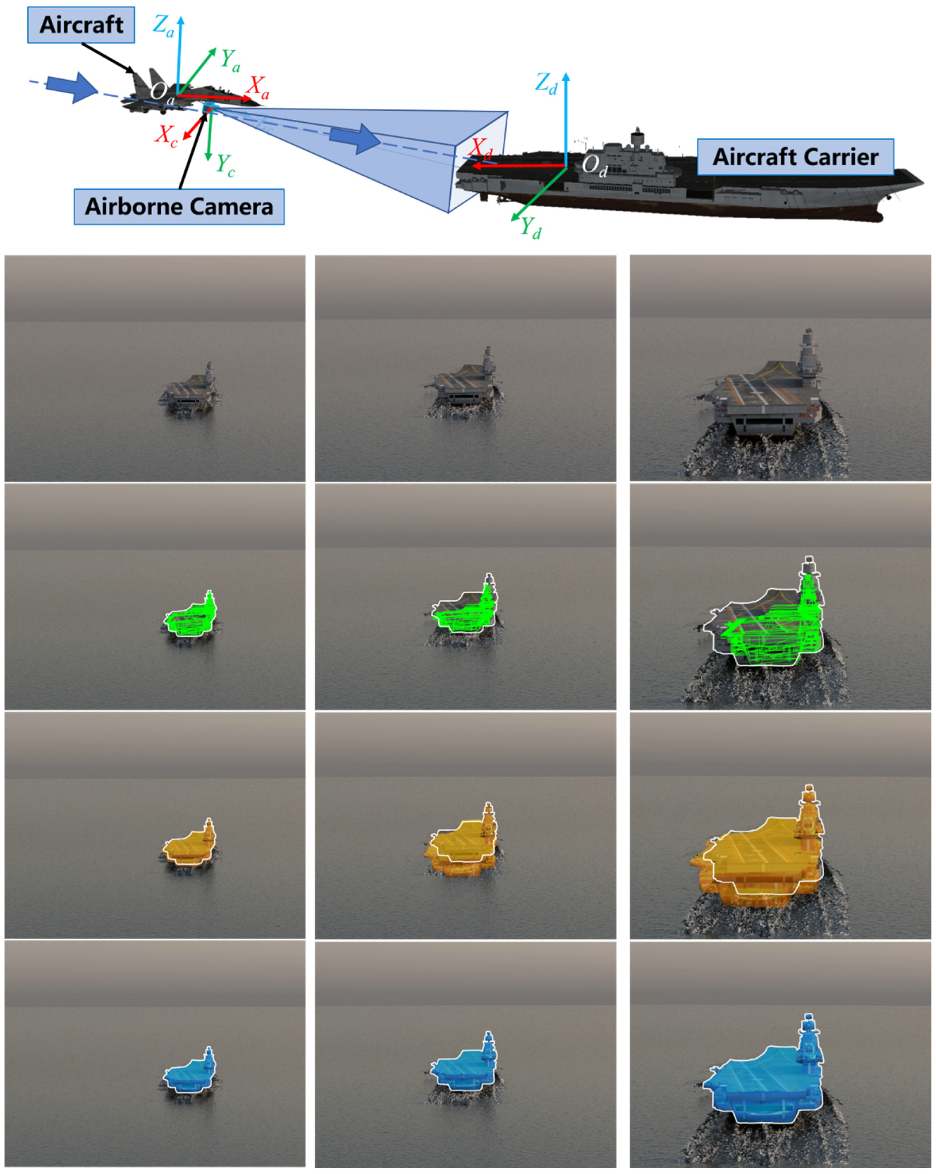
1. Introduction

As a necessary means to guarantee the onboard performance of carrier-borne aircrafts, automatic landing technology plays a crucial role in promoting the development of the carrier-borne aircraft [1]. Traditional landing guidance systems mainly rely on inertial navigation, radar navigation, satellite navigation, and photoelectric navigation. These methods require the support of carrier-borne equipment and aircraft–carrier communication link, which are easy to be interfered with, leading to guidance delay or even failure in complex electromagnetic environment.

Thanks to the rapid development of machine vision in recent years, visual landing has gradually emerged and has become one of the important means of automatic carrier landing [2]. According to different installation positions of the camera, visual guidance methods can be divided into carrier-borne visual guidance method and airborne visual guidance method [3]. The airborne visual landing guidance method mainly relies on the image acquisition and processing equipment carried on the carrier-borne aircraft to complete the calculation of the relative pose parameters between the carrier deck and the aircraft. Then, the guidance information is transmitted to the aircraft control system, so as to realize the autonomous navigation of the aircraft. Independent from the support of the radar, photoelectric, and other external equipment, the landing guidance method based on airborne vision has the advantages of simple structure, strong autonomy, high precision, and electromagnetic interference resistance.

Due to the large distance span of landing process, airborne monocular vision is generally adopted in airborne visual landing guidance schemes. Many researchers have carried out relevant work, which can be summarized into two categories: the cooperative mode and the non-cooperative mode. In the cooperative mode, cooperative signs are arranged on the carrier deck, such as corner reflex mirror cross array [4], infrared cooperative sign lamp array [5,6], infrared cooperative sign circle array [7], T-shaped infrared thermal radiation sign [8], and other asymmetric cooperative signs [9,10]. By extracting point and line features of cooperative signs, the relative pose between the aircraft and the carrier are calculated according to the geometric characteristics and imaging relationship of the cooperative sign so as to guide the aircraft. The guidance methods based on the cooperative sign require the installation of additional signs such as light array on the carrier deck, which will introduce modification to the original design of the carrier deck with poor concealment. When the fixed-wing carrier-borne aircraft is landing, the angle between the optical axis of the airborne camera and the deck surface is small. As the light array arranged in the carrier deck area is narrow, the distribution of cooperative sign lights arranged on the deck is extremely compact in the image, which makes it difficult to solve the pose. Therefore, this paper focuses on the non-cooperative guidance mode based on airborne monocular vision.

The existing research work using non-cooperative mode mainly relies on the carrier’s own characteristics to solve the pose, such as carrier deck runway line features [11,12,13], structural point/line features in the carrier’s interior [14,15], etc. However, the carrier-borne aircraft landing process can be started from as far as more than 5 kilometers. For precise guidance, the runway line or internal structure features in images need to be clearly visible, making these methods [11,12,13,14,15] unable to adapt to the large distance span. In robotic operation, which is a similar application scenario involving large-span visual guidance, a monocular pose tracking method based on the target’s own 3D model information is often used to guide the manipulator to grasp objects [16]. The non-cooperative carrier-guiding process based on airborne monocular vision mainly includes the carrier target detection, the carrier pose detection, and the carrier pose tracking. This paper focuses on the pose tracking part, aiming to propose a monocular pose tracking method merely based on the 3D model of the carrier to track carrier target pose parameters with high precision and stability.

According to the different image information used, the existing 3D-model-based monocular pose tracking methods can be classified into four categories [17]: direct method, feature-based method, edge-based method, and region-based method. In the direct method [18], the photometric consistency of continuous frames is the basis, and the pose change of the target is estimated through direct image alignment. Therefore, this method is extremely sensitive to dynamic light, noise, etc. For feature-based pose tracking methods, sufficient and clear textures are needed to provide robust feature points or feature lines [19]. However, when the carrier-borne aircraft is far away from the carrier, the carrier target in the airborne camera image is too small for this method to be applied. The edge-based method [20,21] generally samples a group of control points along the projected edge of a 3D model. Then, a 1D search is conducted on each sampling point along the normal direction to determine the corresponding relationship. The pose is tracked by minimizing the distance between the sampling edge point and its corresponding point. The region-based method [22,23,24] combines pose tracking with image segmentation. The pose parameters are optimized iteratively to maximize the segmentation energy. The region-based method performs well in dealing with clutter background, dynamic illumination, motion blur, and defocus. In the process of automatic landing guidance of carrier-borne aircraft, the aircraft gradually approaches the carrier target from a far end. Affected by the change of visual range, the carrier target in airborne imaging varies greatly in the whole process, as shown in Figure 1. Both the edge-based GOS algorithm [21] and the traditional region-based RBOT algorithm [24] fail to track the carrier in the scenario of large visual range changes in the landing application.

Aiming at the problems illustrated above, this paper proposes a pose tracking algorithm based on scale-adaptive local region to stably track the pose of carrier target with large scale changes in the process of landing with large range span. The proposed method adopts the non-cooperative mode only using the 3D model of the carrier target, relying on the information of the local regions on the peripheral contour of the carrier, which is most stable in the landing process. The proposed method gives full consideration to the scale change of the carrier target, adaptively updating local region model parameters to realize robust pose tracking of the carrier target under the interference of wave background, sea reflection, and imaging blur.

The contributions of this paper are as follows: (1) A new monocular pose tracking method based on scale-adaptive local region is proposed, which achieves robust pose tracking for the carrier target with large scale variation in landing application scenarios, and achieves better performance than existing algorithms. (2) An innovative updating mechanism of local region model parameters, considering the target scale change in the image, is established to better maintain the continuity of color histogram distribution of the sampled local region near the target contour in continuous frames.

2. Scale-Adaptive Local Region-Based Monocular Pose Tracking Method

Focusing on the application of visual guidance for carrier-borne aircraft landing, this paper proposes a scale-adaptive local region-based pose tracking method to solve the problem of robust 6D pose tracking of the carrier target in the large range span scenario. As shown in Figure 2, on the premise that initial pose is given, firstly, the 2D contour of the carrier is rendered based on its 3D model with the initial pose. Then, a number of circular local regions are established from the uniformly sampled 2D image points on the projected contour. Meanwhile, the local region radius parameters are adjusted according to the pixel scale of the projected contour. Thus, a scale-adaptive local region pose tracking model constrained by pose parameters is constructed. Finally, the pose parameters are solved by iterative optimization so as to optimize the segmentation of the carrier target by maximizing the energy function and the 6D pose tracking of the carrier target in the consecutive frames with the cycle repeating.

In this section, the 6D pose tracking problem of the carrier is described in detail first. Then, the proposed pose tracking model based on scale-adaptive local region is introduced. Finally, the pose optimization solution process is deduced for the energy function.

2.1. Monocular Pose Tracking Problem

In the monocular pose tracking problem, the initial pose of the carrier is considered to be given. With the 3D CAD model of the carrier target, the problem is to continuously estimate and update the 6D pose of the target in the subsequent video frames. Monocular pose tracking is shown in Figure 3. The carrier’s 3D CAD model used in this paper is a dense surface model (triangular mesh) composed of 3D vertices, which can be expressed as ${\mathit{X}}_m={\left(\begin{array}{ccc}{\mathit{x}}_m,& {\mathit{y}}_m,& {\mathit{z}}_m\end{array}\right)}^{\mathrm{T}}\in {ℝ}^3,m=1,\dots ,n$.

In Figure 3, $\mathit{I}$ stands for the input image. $\mathit{T}$ is the rigid body transformation matrix from model coordinate $O_{\mathit{W}}-{\mathit{X}}_{\mathit{W}}{\mathit{Y}}_{\mathit{W}}{Z}_{\mathit{W}}$ to the camera coordinate $O_{\mathit{C}}-{\mathit{X}}_{\mathit{C}}{\mathit{Y}}_{\mathit{C}}{Z}_{\mathit{C}}$, which is defined by rotation matrix $\mathit{R}\in \mathbb{S}\mathbb{O}(3)$ and translation vector $\mathit{t}\in {ℝ}^3$.

$$\mathit{T}=\left[\begin{array}{cc}\mathit{R}& \mathit{t}\\ \mathbf{0}& 1\end{array}\right]\in \mathbb{S}\mathbb{E}(3)$$

(1)

In the continuous image sequence, the rigid body transformation matrix changes constantly with the movement of the model relative to the camera, and pose tracking is actually an iterative update of the transformation matrix. If the pose of the k-th frame is ${\mathit{T}}_{\mathit{k}}=\mathsf{\Delta }\mathit{T}{\mathit{T}}_{\mathit{k}-1}$, $\mathsf{\Delta }\mathit{T}={\mathit{T}}_{\mathit{k}}{\mathit{T}}_{{}_{\mathit{k}-1}}^{-1}$ is the pose update from the previous frame to the k-th frame. During pose tracking, the pose of each frame can be obtained merely by calculating the pose update between frames. In order to facilitate the nonlinear optimization of the transformation matrix solution in continuous frames, the transformation matrix is represented by 6D pose vector $\mathit{p}$, represented by Lie algebra [25].

$$\mathit{p}=\left[\begin{array}{c}\mathit{w}\\ \mathit{v}\end{array}\right]={({\omega }_1,{\omega }_2,{\omega }_3,v_1,v_2,v_3)}^{\mathrm{T}}\in {ℝ}^6$$

(2)

The pose update of Lie algebra pose vector $\widehat{\mathit{p}}$ is mapped to the transformation matrix $\mathsf{\Delta }\mathit{T}$ as follows:

$$\mathsf{\Delta }\mathit{T}=\exp (\widehat{\mathit{p}})\in \mathbb{S}\mathbb{E}(3), \widehat{\mathit{p}}=\left[\begin{array}{cc}\widehat{\mathit{w}}& \mathit{v}\\ \mathbf{0}& 0\end{array}\right]\in se(3),\widehat{\mathit{w}}\in so(3),\mathit{v}\in {ℝ}^3$$

(3)

where $\widehat{\mathit{w}}=\left[\begin{array}{ccc}0& -{\mathit{w}}_3& {\mathit{w}}_2\\ {\mathit{w}}_3& 0& -{\mathit{w}}_1\\ -{\mathit{w}}_2& {\mathit{w}}_1& 0\end{array}\right]$ is the corresponding antisymmetric matrix of $\mathit{w}$.

Assume that the camera has been pre-calibrated and its intrinsic parameters are fixed. The intrinsic parameter matrix $\mathit{K}$ is shown below:

$$\mathit{K}=\left[\begin{array}{ccc}{\mathit{f}}_{\mathit{x}}& 0& {\mathit{C}}_{\mathit{x}}\\ 0& f_{\mathit{y}}& {\mathit{C}}_{\mathit{y}}\\ 0& 0& 1\end{array}\right]\in {ℝ}^{3\times 3}$$

(4)

After nonlinear distortion correction, the input image is considered undistorted. Perspective projection from 3D vertices to 2D image points can be described as

$$\mathit{x}=\pi \left(\mathit{K}{\left(\mathit{T}\tilde{\mathit{X}}\right)}_{3\times 1}\right)$$

(5)

where $\mathit{x}$ is the 2D projected point of the 3D model vertex $\mathit{X}$. $\tilde{\mathit{X}}={\left(\mathit{x},\mathit{y},z,1\right)}^{\mathrm{T}}$ is the homogeneous extension of $\mathit{X}={(\mathit{x},\mathit{y},z)}^{\mathrm{T}}={(\tilde{\mathit{X}})}_{3\times 1}$, and $\pi \left(\mathit{X}\right)={(\mathit{x}/\mathit{z},\mathit{y}/\mathit{z})}^{\mathit{T}}$. Based on the initial pose, the projection mask $I_s$ is generated by rendering the 3D model. Then, the whole image can be divided into foreground region and background region by extracting the contour on the projection mask. Constrained by the 3D model of the carrier target, when the 6D pose parameters are correct, the projected contour $\mathit{C}$ can perfectly segment the carrier target in the image.

2.2. Pose Tracking Model based on Scale-Adaptive Local Region

In the case of a given initial pose, region-based monocular pose tracking updates the transformation matrix ${\mathit{T}}_{\mathit{k}}$ by continuously solving the pose change $\mathsf{\Delta }\mathit{T}$ in successive frames. Existing region-based methods adopt a fixed local region model parameter, which is difficult to adapt to the application concerned in this paper. In view of this, a new pose tracking model based on scale-adaptive local region is proposed. The specific structure of the proposed model is shown in Figure 4. For the local region-based method, the target in the image is represented by the level set embedding function (or signed distance function), as shown in Equation (6). The signed distance function $\mathsf{\Phi }(\mathit{x})$ computes the (signed) Euclidean distance between a pixel $\mathit{x}$ in an image and its nearest contour point. Then, the projected contour $\mathit{C}$ is defined as a set of zero elevation points $\mathit{C}=\left\{\mathit{x}|\mathsf{\Phi }(\mathit{x})=0\right\}$.

$$\mathsf{\Phi }(\mathit{x})=\{\begin{array}{c}-\mathit{d}(\mathit{x},\mathit{C}),\forall \mathit{x}\in {\mathsf{\Omega }}_f\\ \mathit{d}(\mathit{x},\mathit{C}),\forall \mathit{x}\in {\mathsf{\Omega }}_b\end{array}$$

(6)

where, $\mathit{d}(\mathit{x},\mathit{C})=\underset{\mathit{c}\in \mathit{C}}{\min }{\Vert \mathit{c}-\mathit{x}\Vert }_2$.

We define the region of $\mathsf{\Phi }(\mathit{x})<0$ in the image as the foreground region ${\mathsf{\Omega }}_f$, while the region of $\mathsf{\Phi }(\mathit{x})>0$ is the background region ${\mathsf{\Omega }}_b$, and the foreground and the background regions are divided by the projected contour $\mathit{C}$, as shown in the left graph of “Local Region Establishing” in Figure 4. In order to ensure the correspondence of local regions in the image sequence, we screen the region centers ${\mathit{x}}_{{\mathit{C}}_i}$ in the 3D vertices ${\mathit{X}}_m$ of the target model near the projected contour $\mathit{C}$. The regional centers are selected to be as evenly distributed as possible on the contour, so as to determine the local circular regions ${\mathsf{\Omega }}_i$. Local circular regions ${\mathsf{\Omega }}_i$ are then divided into the foreground part ${\mathsf{\Omega }}_{f_i}$ and the background part ${\mathsf{\Omega }}_{b_i}={\mathsf{\Omega }}_i\backslash {\mathsf{\Omega }}_{f_i}$. For each local region ${\mathsf{\Omega }}_i$, the foreground and background statistical characteristics in the region are usually represented by foreground color appearance model $\mathit{P}\left(\mathit{y}\mid M_{f_i}\right)$ and background color appearance model $\mathit{P}\left(\mathit{y}\mid M_{b_i}\right)$, where $\mathit{y}=I(\mathit{x})$ is the RGB value of a pixel $\mathit{x}$ in the image. The color appearance models describe the probability that the pixel color $\mathit{y}$ meets the color distribution of the foreground local region and the background local region, respectively, which are represented by the region RGB color histogram, as shown in the right graph of "Local Region Establishing" in Figure 4.

For each local region, counting the foreground/background color appearance model of the region, the posterior probability of local area pixels can be obtained, which is calculated as follows:

$${\mathit{P}}_{{\mathit{f}}_{\mathit{i}}}(\mathit{x})=\mathit{P}\left({\mathit{M}}_{{\mathit{f}}_{\mathit{i}}}\mid \mathit{y}\right)=\frac{\mathit{P}\left(\mathit{y}\mid {\mathit{M}}_{{\mathit{f}}_{\mathit{i}}}\right)}{{\eta }_{{\mathit{f}}_{\mathit{i}}}\mathit{P}\left(\mathit{y}\mid {\mathit{M}}_{{\mathit{f}}_{\mathit{i}}}\right)+{\eta }_{{\mathit{b}}_{\mathit{i}}}\mathit{P}\left(\mathit{y}\mid {\mathit{M}}_{{\mathit{b}}_{\mathit{i}}}\right)}$$

(7)

$${\mathit{P}}_{{\mathit{b}}_{\mathit{i}}}(\mathit{x})=\mathit{P}\left({\mathit{M}}_{{\mathit{b}}_{\mathit{i}}}\mid \mathit{y}\right)=\frac{\mathit{P}\left(\mathit{y}\mid {\mathit{M}}_{{\mathit{b}}_{\mathit{i}}}\right)}{{\eta }_{{\mathit{f}}_{\mathit{i}}}\mathit{P}\left(\mathit{y}\mid {\mathit{M}}_{{\mathit{f}}_{\mathit{i}}}\right)+{\eta }_{{\mathit{b}}_{\mathit{i}}}\mathit{P}\left(\mathit{y}\mid {\mathit{M}}_{{\mathit{b}}_{\mathit{i}}}\right)}$$

(8)

where

$${\eta }_{f_i}=\sum _{\mathit{x}\in {\mathrm{\Omega }}_i}{H}_e(\mathrm{\Phi }(\mathit{x})),{\eta }_{b_i}=\sum _{\mathit{x}\in {\mathrm{\Omega }}_i}\left(1-H_e(\mathsf{\Phi }(\mathit{x}))\right)$$

(9)

$$H_e(\mathsf{\Phi }(\mathit{x}))=\frac{1}{\pi }\left(-atan(s\cdot \mathsf{\Phi }(\mathit{x}))+\frac{\pi }{2}\right)$$

(10)

$P_{f_i}(\mathit{x})$ and $P_{b_i}(\mathit{x})$ are the foreground pixelwise posterior probability and the background pixelwise posterior probability of the pixel $\mathit{x}$ in the $i$-th local region ${\mathsf{\Omega }}_i$, respectively. $H_e$ is a smoothed Heaviside step function. $s$ is the slope index; here, $s=1.2$.

In the iteration of pose parameters in the consecutive frame sequence, the color histogram of the foreground and background corresponding to the local region of the same center ${\mathit{x}}_{{\mathit{C}}_i}$ possesses continuity in the adjacent frames. Based on this, we refer to the recursive updating strategy of region appearance model in [13,15] in the practical implementation. After the (k-1)-th frame is successfully tracked, the color appearance models $P^{\mathit{K}}\left(\mathit{y}\mid M_{f_i}\right)$ and $P^{\mathit{K}}\left(\mathit{y}\mid M_{b_i}\right)$ of the local background in the k-th frame are established as partial inheritance of the color appearance model of the corresponding region in the previous frame, and the update strategy is as follows:

$$P^{\mathit{k}}\left(\mathit{y}\mid M_{f_i}\right)=\left(1-{\alpha }_f\right)P^{\mathit{k}-1}\left(\mathit{y}\mid M_{f_i}\right)+{\alpha }_f{P}^{\mathit{k}}\left(\mathit{y}\mid M_{f_i}\right)$$

(11)

$$P^{\mathit{k}}\left(\mathit{y}\mid M_{b_i}\right)=\left(1-{\alpha }_b\right)P^{\mathit{k}-1}\left(\mathit{y}\mid M_{b_i}\right)+{\alpha }_b{P}^{\mathit{k}}\left(\mathit{y}\mid M_{b_i}\right)$$

(12)

${\alpha }_f$ and ${\alpha }_b$ are the learning rate of the foreground region and background region. To effectively cope with imaging jitter and avoid the jump of pose parameters to improve the tracking result, we set ${\alpha }_f=0.1$, ${\alpha }_b=0.2$.

In the fusion of statistical models of all local regions, pixels near the target contour will belong to several local regions at the same time due to the overlap between different local regions. Similar to [15], we choose to calculate the average posterior probability of pixels in all local regions to which they belong. In the k-th frame, for each pixel $\mathit{x}$ in the image, the mean posterior probability of foreground and mean posterior probability of background are calculated as follows:

$${\overline{P}}_f^{\mathit{k}}(\mathit{x})=\frac{1}{{\sum }_{i=1}^n{\mathrm{B}}_i^{\mathit{k}}(\mathit{x},{\mathit{x}}_{{\mathit{C}}_i})}\sum _{i=1}^n{P}_{f_i}^{\mathit{k}}(\mathit{x}){\mathrm{B}}_i^{\mathit{k}}(\mathit{x},{\mathit{x}}_{{\mathit{C}}_i})$$

(13)

$${\overline{P}}_b^{\mathit{k}}(\mathit{x})=\frac{1}{{\sum }_{i=1}^n{\mathrm{B}}_i^{\mathit{k}}(\mathit{x},{\mathit{x}}_{{\mathit{C}}_i})}\sum _{i=1}^n{P}_{b_i}^{\mathit{k}}(\mathit{x}){\mathrm{B}}_i^{\mathit{k}}(\mathit{x},{\mathit{x}}_{{\mathit{C}}_i})$$

(14)

where

$${\mathrm{B}}_i^{\mathit{k}}(\mathit{x},{\mathit{x}}_{{\mathit{C}}_i})=\{\begin{array}{c}1,\left|\mathit{x}-{\mathit{x}}_{{\mathit{C}}_i}\right|<r^{\mathit{k}}\\ 0,\hspace{1em}\hspace{1em}\hspace{1em}else\hfill \end{array}$$

(15)

$r^{\mathit{k}}$ is the radius of the local region ${\mathsf{\Omega }}_i^{\mathit{k}}$ in the k-th frame. ${\mathit{x}}_{{\mathit{C}}_i}$ is the corresponding region center.

In order to adapt to the change of carrier target scale caused by the variation of visual distance between carrier target and airborne camera, the size of the local region is set to increase with the increase of target scale to maintain the continuity of foreground background sampling in the image sequence within the regions. Too-small region radius will not be able to cope with large target pose changes, while too-large area radius will lead to poor pose convergence accuracy. Therefore, the adjustment of the region radius needs to be within a certain range. Considering the complexity of the 3D structure of the carrier target, the target scale is defined as the pixel length of the shorter side of the minimum enclosing rectangle of the target’s projected contour. Assuming that the carrier target is successfully tracked, the target scales in adjacent frames can be regarded as approximately unvaried. First, the target scales of the carrier target in the previous frame are detected, as shown in the “Region Radius Updating” part in Figure 4. Then, according to the detected target scale, the region parameters are updated in the pose optimization of the current frame.

Sigmoid function is utilized to design the updating mechanism of radius parameters, which can not only limit the variation range of region radius, but also ensure the approximate linear relationship between local region radius and the change of target scale within a certain range. The specific form is as follows:

$$r^{\mathit{k}}=\frac{\mathit{c}}{1+e^{-a\left[\min \left({\mathit{w}}^{\mathit{k}-1},h^{\mathit{k}-1}\right)-b\right]}}+d$$

(16)

${\mathit{w}}^{\mathit{k}-1}$ and $h^{\mathit{k}-1}$ are the width and height of the minimum enclosing rectangle of the projected contour of the target 3D model in the (k-1)-th frame. a is the sensitivity coefficient. b is the scale offset. The higher the sensitivity coefficient is, the more drastic the radius changes with the target scale. The sensitivity coefficient is normally set between 0.02 to 0.2. Here, $a=0.04,b=150$. c is the length of radius variation interval, and d is the minimum radius parameter. Here, according to the specific application scenario, the radius change interval is set at [10, 70].

Then, the local region-based energy function for pose tracking can be expressed as

$$E(\mathit{p})=-\sum _{\mathit{x}\in \mathrm{\Omega }}\log \left[H_e(\mathsf{\Phi }(\mathit{x}(\mathit{p}))){\bar{P}}_f(\mathit{x})+\left(1-H_e(\mathsf{\Phi }(\mathit{x}(\mathit{p})))\right){\bar{P}}_b(\mathit{x})\right]$$

(17)

This energy function takes the target pose parameters $\mathit{p}$ as independent variables and quantitatively describes the target segmentation performance under the constraints of the 3D model, that is, the degree of coincidence between the rendered 2D template and the target region in the image. When the energy is maximum, the segmentation result of the target region is best.

2.3. Pose Optimization

According to the construction of energy function given in Section 2.2, in order to solve the optimal pose, this paper adopts the Gauss–Newton pose optimization method to solve this complex nonlinear optimization problem by referring to [24]. First, Equation (17) is reconstructed into a nonlinear iterative reweighted least squares problem of the following form:

$$E(\mathit{p})=\frac{1}{2}\sum _{\mathit{x}\in \mathsf{\Omega }}\psi (\mathit{x})F^2(\mathit{x},\mathit{p})$$

(18)

where

$$F(\mathit{x},\mathit{p})=-\log [H_e(\mathsf{\Phi }(\mathit{x}(\mathit{p}))){\overline{\mathit{P}}}_f(\mathit{x})+\left(1-H_e(\mathsf{\Phi }(\mathit{x}(\mathit{p})))\right){\overline{\mathit{P}}}_b(\mathit{x})], \psi (\mathit{x})=\frac{1}{F(\mathit{x},\mathit{p})}$$

(19)

In order to optimize the energy function, we first consider the weight coefficient $\psi (\mathit{x})$ as the fixed weight and use the Gauss–Newton method to solve the pose parameters $\mathit{p}$, then use the optimized pose parameters $\mathit{p}$ to calculate the weight coefficient $\psi (\mathit{x})$ to update the weight value and enter the next iterative solution.

Under the assumption of fixed weights, the derivative of the energy function with respect to the pose $\mathit{p}$ is obtained, and the gradient function is as follows:

$$\begin{array}{l}\frac{\delta E(\mathit{p})}{\delta \mathit{p}}=\frac{1}{2}{\displaystyle \sum _{\mathit{x}\in \mathsf{\Omega }}}\psi (\mathit{x})\frac{\delta F^2(\mathit{x},\mathit{p})}{\delta \mathit{p}}\\ ={\displaystyle \sum _{\mathit{x}\in \mathsf{\Omega }}}\psi (\mathit{x})F(\mathit{x},\mathit{p})\frac{\delta F(\mathit{x},\mathit{p})}{\delta \mathit{p}}\end{array}$$

(20)

Since $\psi (\mathit{x})F(\mathit{x},\mathit{p})=1$, the Jacobian is computed as follows:

$$\begin{array}{l}\mathit{J}(\mathit{x})=\frac{\partial F(\mathit{x},\mathit{p})}{\partial \mathit{p}}\\ =-\frac{{\overline{\mathit{p}}}_f-{\overline{\mathit{p}}}_b}{H_e(\mathsf{\Phi }(\mathit{x})){\overline{\mathit{p}}}_f+\left(1-H_e(\mathsf{\Phi }(\mathit{x}))\right){\overline{\mathit{p}}}_b}\times \frac{\partial H_e(\mathsf{\Phi }(\mathit{x}))}{\partial \mathit{p}}\end{array}$$

(21)

$$\frac{\partial H_e(\mathsf{\Phi }(\mathit{x}))}{\partial \mathit{p}}=\frac{\partial H_e}{\partial \mathsf{\Phi }}\frac{\partial \mathsf{\Phi }}{\partial \mathit{x}}\frac{\partial \mathit{x}}{\partial \mathit{p}}$$

(22)

in which, $\frac{\partial H_e}{\partial \mathsf{\Phi }}={\delta }_e(\mathsf{\Phi })$ is the smoothed Dirac function. According to Equation (10),

$${\delta }_e(\mathsf{\Phi }(\mathit{x}))=\frac{\partial H_e(\mathsf{\Phi }(\mathit{x}))}{\partial \mathsf{\Phi }}=-\frac{s}{\pi \left(1+s^2{\mathsf{\Phi }}^2(\mathit{x})\right)}$$

(23)

For the derivative of the level set embedding function with respect to pixel position $\frac{\partial \mathsf{\Phi }}{\partial \mathit{x}}$, the central difference method is used:

$$\frac{\partial \mathsf{\Phi }}{\partial \mathit{x}}=\left[\frac{\partial \mathsf{\Phi }}{\partial x},\frac{\partial \mathsf{\Phi }}{\partial y}\right]={\left[\begin{array}{l}\frac{\mathsf{\Phi }(x+1,y)-\mathsf{\Phi }(x-1,y)}{2}\\ \frac{\mathsf{\Phi }(x,y+1)-\mathsf{\Phi }(x,y-1)}{2}\end{array}\right]}^{\mathrm{T}}$$

(24)

Since $\mathit{x}(\mathit{p})=\pi \left(\mathit{K}{\left(\exp (\widehat{\mathit{p}})\mathit{T}\tilde{\mathit{X}}\right)}_{3\times 1}\right)$, $\frac{\partial \mathit{x}}{\partial \mathit{p}}$ can be deduced. Suppose that after tiny motion, we perform piecewise linearization of the matrix exponential in each iteration, and obtain $\exp (\widehat{\mathit{p}})\approx I_{4\times 4}+\widehat{\mathit{p}}$:

$$\begin{array}{l}\frac{\partial \mathit{x}}{\partial \mathit{p}}=\frac{\partial \pi }{\partial \mathit{K}{(\exp (\widehat{p})\mathit{T}\tilde{\mathit{X}})}_{3\times 1}}\frac{\partial \mathit{K}{(\exp (\widehat{\mathit{p}})\mathit{T}\tilde{\mathit{X}})}_{3\times 1}}{\partial p}\\ =\left[\begin{array}{c}\begin{array}{ccc}\frac{f_{\mathit{x}}}{z^{\prime }}& 0& -\frac{{\mathit{x}}^{\prime }{f}_{\mathit{x}}}{{(z^{\prime })}^2}\end{array}\\ \begin{array}{ccc}0& \frac{f_{\mathit{y}}}{z^{\prime }}& -\frac{{\mathit{y}}^{\prime }{f}_{\mathit{y}}}{{(z^{\prime })}^2}\end{array}\end{array}\right]\cdot \left[\begin{array}{c}\begin{array}{cccccc}0& z^{\prime }& -{\mathit{y}}^{\prime }& 1& 0& 0\end{array}\\ \begin{array}{cccccc}-z^{\prime }& 0& {\mathit{x}}^{\prime }& 0& 1& 0\end{array}\\ \begin{array}{cccccc}{\mathit{y}}^{\prime }& -{\mathit{x}}^{\prime }& 0& 0& 0& 1\end{array}\end{array}\right]\end{array}$$

(25)

where ${\mathit{X}}^{\prime }={({\mathit{x}}^{\prime },{\mathit{y}}^{\prime },{\mathit{z}}^{\prime })}^{\mathrm{T}}={(\mathit{T}\tilde{\mathit{X}})}_{3\times 1}$.

Through the derivation of the partial derivatives of the items in the Jacobian matrix above, the Hessian matrix and the pose change can be obtained as follows,

$$\mathit{H}(\mathit{x})=\psi (\mathit{x})\mathit{J}{(\mathit{x})}^{\mathrm{T}}\mathit{J}(\mathit{x})$$

(26)

$$\mathrm{\Delta }p=-{\left(\sum _{\mathit{x}\in \mathrm{\Omega }}\mathit{H}(\mathit{x})\right)}^{-1}\sum _{\mathit{x}\in \mathrm{\Omega }}\mathit{J}(\mathit{x}{)}^{\mathrm{T}}$$

(27)

By iteratively solving the pose update $\mathsf{\Delta }\mathit{p}$ for each input frame of the image sequence, the pose tracking of the target is realized.

3. Experimental Evaluation

3.1. Experiment Setting

To validate the pose tracking performance of the proposed method in this paper on the carrier target, this section simulates the imaging of the carrier target by the airborne camera in the process of carrier landing. During landing, the flight attitude of the carrier-borne aircraft needs to be controlled with high precision. In order to ensure a smooth landing and a successful rope hanging, the aircraft flies at a fixed angle of descent, which is around 3–5°, to maintain the angle of attack. Based on this, this section uses a synthetic simulation image sequence generated by a simulation rendering software 3Ds max and a real image sequence captured through a scale physical simulation system to verify the effectiveness of the proposed algorithm in this paper.

We compared the proposed algorithm with the existing representative region-based pose tracking method RBOT algorithm [24] and the edge-based pose tracking method GOS algorithm [21] on the two image sequences, respectively. For the comparison algorithms, we adopted the default parameter settings suggested in their papers. All experiments were carried out on a laptop equipped with an AMD Ryzen 7 4800H processor (8-core) @ 2.9 GHz, NVIDIA GeForce GTX1650 GPU and 16 GB RAM. The GPU was only used for the rendering of the 3D model. The rest of the algorithm runs on the CPU. The proposed algorithm is implemented in C++. For the synthetic image sequence with a resolution of 800 × 600 and the real image sequence with a resolution of 800 × 800, the proposed algorithm can reach the processing speed of 30 fps, which can basically meet the requirements of high efficiency of real-time pose tracking for the carrier target in the process of carrier-borne aircraft landing.

3.2. Experiment on Synthetic Image Sequence

This section uses simulation rendering software to generate a synthetic image sequence to simulate the imaging of the carrier target by airborne camera during the landing process. To quantitatively measure the pose tracking accuracy, the metrics and corresponding results and analysis are given in this section.

3.2.1. Synthetic Sequence Settings

The simulation software used in this section is Autodesk 3Ds Max, which is often used in 3D modeling, animation, and scene rendering. In the simulation rendering of carrier-borne aircraft landing, the carrier’s 3D model is the “Varyag” model downloaded on the internet.

Table 1. Parameter settings in 3Ds Max simulation.

3D Model Size	Focal Length	Field Angle	Frame Size
94.36 m × 66.01 m × 304.51 m	12 mm	24° × 18°	800 × 600

shows the 3D model size parameters and 3Ds Max simulation parameters.

Through the settings of the virtual camera parameter and its trajectory, as well as the rendering of the of dynamic sea surface scene including dynamic light, sea waves, and sea horizon simulation, we generated an image sequence consisting of 350 frames. The synthetic sequence simulates aircraft approaching the ship deck from about 1120 m. With the shortening of the distance, the ship target in the image becomes larger and larger, with the details of the ship target clearer and clearer. The camera intrinsic parameters $\mathit{K}$, initial pose ${\mathit{T}}_0$, and the ship 3D model were used as input to initialize the pose tracking algorithm. The proposed algorithm optimizes the pose variation of the ship target between successive frames by establishing local region models on the projected contour of the 3D model to maximize the energy function for the optimal segmentation, so that the pose parameters of the ship target can be continuously solved in the image sequence to achieve pose tracking. Examples of the synthetic images (the 2nd, 147th, 208th, 290th, and 335th frames) are shown in the first row of the upper half in Figure 5.

3.2.2. Experimental Results and Analysis

For visualization, the reprojected mask and the pose curves of the pose tracking results are presented in Figure 5. The second to fourth rows are the reprojected results of GOS algorithm [21], RBOT algorithm [24], and the proposed algorithm for the ship target pose tracking. The bottom part of Figure 5 shows the pose curves of the three algorithms. As can be seen from Figure 5, in the synthetic image sequence, the proposed method achieved whole-process stable pose tracking of the ship target. Owing to the ship target’s complex interior structure, and its low color distinctiveness under the background of dynamic sea surface, the GOS algorithm [21] failed to track the pose of the ship from the fifth frame when the ship target is small. With the pose error accumulated in the process of tracking, although the target increased gradually, the pose tracking result kept becoming worse. The GOS algorithm [21] searches the corresponding points between frames on the normal line segment for discrete points at the edge of the ship target. This method is based on edge features, and strongly relies on the gradient information on the normal line segment to achieve stable pose tracking for untextured or weakly textured targets. For the ship target with complex internal textures, the 1D search on the normal lines in the GOS algorithm [21] is easily disturbed by the maximum value of internal gradient response, resulting in mismatching and errors in pose solution. The RBOT algorithm [24] also tended to fail tracking in the first five frames of the image sequence. However, according to the reprojected results, the problem centered on the segmentation of the stern part of the ship target, while the segmentation of the bow and tower part behaved well. Firstly, the interference of the aft waves of the ship weakens the foreground–background distinctiveness in the stern regions. Secondly, although the RBOT algorithm [24] applies the region features around the target contour, it adopts the local regions with fixed radius, which fails to adapt to the scale variation of the ship target in the landing application.

Aiming at the specific scenario for carrier landing, we considered the scale variation of the ship target caused by drastic changes in visual range. The proposed pose tracking method adaptively adjusts the local region radius parameter according to the scale of the ship target in the image, ensuring the continuity of the color histograms of corresponding local regions between adjacent frames. In this way, the energy function optimization in image sequence achieves better target segmentation effect by using the continuity information between frames more effectively. Figure 6 shows the process of local region radius adjustment with ship target scale. When the ship target is small, the smaller region radius segments the ship more accurately in terms of the wave background interference. When the scale of the ship target gradually largens with the decrease of the visual distance, the proposed algorithm increases the region radius to better maintain the color distribution characteristics of the front background in the local regions along the contour. As shown in Figure 5, the blue reprojected mask corresponds to the ship target in the whole process. Additionally, pose curves coincide with the ground truth curves. It is indicated that the proposed algorithm realizes robust pose tracking of the ship target, adapting to the target scale changes, the sea background, and the light interference.

To quantify the accuracy of pose tracking results, the pose tracking results of the algorithm were compared with the pose truth value to calculate the angular error $e_R$ and relative position error $e_{\mathit{t}\_rela\mathit{t}ive}$, as shown below:

$${\mathit{e}}_{\mathit{R}}({\mathit{t}}_{\mathit{k}})={\cos }^{-1}\left(\frac{\mathit{t}ra\mathit{c}e(\mathit{R}{({\mathit{t}}_{\mathit{k}})}^{\mathrm{T}}{\mathit{R}}_{G\mathit{T}}({\mathit{t}}_{\mathit{k}})-1}{2}\right)$$

(28)

$$e_{\mathit{t}\_rela\mathit{t}ive}({\mathit{t}}_{\mathit{k}})=\frac{{\Vert \mathit{t}({\mathit{t}}_{\mathit{k}})-{\mathit{t}}_{\mathit{G}\mathit{T}}({\mathit{t}}_{\mathit{k}})\Vert }_2}{{\Vert {\mathit{t}}_{\mathit{G}\mathit{T}}({\mathit{t}}_{\mathit{k}})\Vert }_2}$$

(29)

$\mathit{R}({\mathit{t}}_{\mathit{k}})$ and $\mathit{t}({\mathit{t}}_{\mathit{k}})$ are the rotation matrix and translation vector of the pose tracking result in ${\mathit{t}}_{\mathit{k}}$ moment.${\mathit{R}}_{\mathit{G}\mathit{T}}({\mathit{t}}_{\mathit{k}})$ and ${\mathit{t}}_{\mathit{G}\mathit{T}}({\mathit{t}}_{\mathit{k}})$ are the ground truth value in ${\mathit{t}}_{\mathit{k}}$ moment.

Since the landing process is a large span approaching process between carrier-borne aircraft and carrier target, the absolute displacement error is greatly affected by the distance, so the relative error is chosen to measure the accuracy. The error of pose tracking results is shown in Figure 7. In the synthetic image sequence test, the angle error of pose tracking of the proposed algorithm is no more than 1° in the whole process, and the relative displacement error does not exceed 1%. Synthetic image sequence experiments verify the effectiveness of the proposed algorithm in pose tracking of the carrier target with high precision during the landing process.

3.3. Experiment on Real Image Sequence

3.3.1. Scale Physical Simulation Platform

In the synthetic image sequence, although the dynamic sea surface scene is simulated, there is still a certain gap between the virtual synthetic images and the practical images taken by the industrial camera, which includes noise interference, defocus blur, and motion blur. In order to further test the performance of the algorithm in the actual image sequence, according to the fixed slide angle setting in real carrier landing, we built the scale simulation sliding platform of the carrier landing, as shown in Figure 8.

The industrial color camera is fixed on the electric slide trolley. One end of the track is close to the seascape sand table with the carrier scale model. The other end is supported on the electric lifting platform. The electric lift platform can adjust the angle of descent of the glide track by changing the height of one end of the track. In this experiment, the track length is about 4 m, and the gliding angle of the track is set as 3°. The ratio of actual carrier size to carrier model is 700:1. The scale simulation parameter settings are shown in

Table 2. Experimental settings of scale simulation.

Carrier Model Scale	Track Length	Focal Length	Frame Rate	Frame Size
700:1	4 m	12 mm	30 fps	800 × 800

.

The CAD model of the carrier model was scanned and reconstructed by high-precision 3D scanning equipment, and the intrinsic parameters of the industrial camera were calibrated in advance using Zhang’s calibration method [26]. A total of 1190 frames of images were captured by the industrial camera during the sliding process of the electric trolley with a constant speed. In order to obtain the initial pose parameters of the carrier target, a number of 2D feature points are selected in the image, and then the corresponding 3D coordinates of the feature points are obtained by using the total station and converting into the carrier model coordinate system. With the 2D–3D points correspondence, the initial pose is solved by the PnP algorithm [27]. Similar to Section 2.2, initial pose and camera intrinsic parameters were used as the input to initialize the algorithm. Since the GOS algorithm [21] performs poorly, we only compare RBOT algorithm with our algorithm in the real image sequence test in this section. The reprojected results and pose curves are shown in Figure 9.

3.3.2. Experimental Results and Analysis

As shown in Figure 9, in the real image sequence of scale physical simulation, the actual imaging is degraded by defocus blur, motion blur, and environmental interference, such as "sea surface" illumination reflection and cluttered background. According to the pose tracking results, the reprojected mask of the proposed algorithm can accurately match the carrier target in the whole process of image sequence. However, for the RBOT algorithm [24], the pose tracking results showed deviation after initialization immediately. As the carrier target gradually become larger, it failed to timely correct the accumulated tracking error, and the pose tracking deviation also further expanded. Figure 10 shows the process of local area radius changing with the carrier target scale. In the real image sequence, due to the large range span, the scale of the carrier target varies from 50 pixels to 600 pixels. The scale variation of the carrier target is larger than that in the synthetic image sequence. In terms of the large scale variation, the proposed algorithm updates the local area radius in real time according to the target scale, and still realizes the whole-process stable 6D pose tracking of the carrier target. The scale physical simulation experiment again verifies the effectiveness of the proposed algorithm in achieving robust pose tracking for the carrier target in carrier landing application.

4. Conclusions

Aiming at the carrier landing scenario with monocular airborne visual guidance, this paper proposes a carrier target pose tracking method based on scale-adaptive local region. By combining the carrier target scale variation characteristics caused by visual distance change in the landing process, a pose tracking model based on local regions is set up with the local region radius updating adaptively. Then, using the Gauss–Newton optimization algorithm, the 6D pose tracking of the carrier target is achieved. Experiments on both synthetic image sequence and real image sequence verify that the proposed method can achieve accurate and robust pose tracking for the carrier target in the process of carrier aircraft approaching and landing from far to near.

References

- Wu, H.; Luo, F.; Shi, X.; Liu, B.; Lian, X. Analysis on the Status Quo and Development Trend of Automatic Carrier Landing Technology. Aircr. Des. 2020, 1–5. (In Chinese) [Google Scholar] [CrossRef]
- Zhen, Z.; Wang, X.; Jiang, J.; Yang, Y. Research progress in guidance and control of automatic carrier landing of carrier-based aircraft. Acta Aeronaut. Astronaut. Sin. 2017, 38, 22. (In Chinese) [Google Scholar]
- Wei, Z. Overview of Visual Measurement Technology for Landing Position and Attitude of Carrier-Based Aircraft. Meas. Control. Technol. 2020, 39, 2–6. (In Chinese) [Google Scholar]
- Xu, G.; Cheng, Y.; Shen, C. Key Technology of Unmanned Aerial Vehicle’s Navigation and Automatic Landing in All Weather Based on the Cooperative Object and Infrared Computer Vision. Acta Aeronaut. Astronaut. Sinica 2008, 2, 437–442. (In Chinese) [Google Scholar]
- Wang, X.-H.; Xu, G.-L.; Tian, Y.-P.; Wang, B.; Wang, J.-D. UAV’s Automatic Landing in All Weather Based on the Cooperative Object and Computer Vision. In Proceedings of the 2012 Second International Conference on Instrumentation, Measurement, Computer, Communication and Control, Harbin, China, 8–10 December 2012. [Google Scholar]
- Gui, Y.; Guo, P.; Zhang, H.; Lei, Z.; Zhou, X.; Du, J.; Yu, Q. Airborne Vision-Based Navigation Method for UAV Accuracy Landing Using Infrared Lamps. J. Intell. Robot. Syst. 2013, 72, 197–218. [Google Scholar] [CrossRef]
- Wang, G.; Li, H.; Ding, W.; Li, H. Technology of UAV Vision-guided Landing on a Moving Ship. J. China Acad. Electron. Inf. Technol. 2012, 7, 274–278. (In Chinese) [Google Scholar]
- Chen, L. Research on the Autonomous Landing Flight Control Technology for UAV Based on Visual Servoing. Master’s Thesis, Nanjing University of Aeronautics and Astronautics, Nanjing, China, 2009. (In Chinese). [Google Scholar]
- Hao, S.; Chen, Y.M.; Ma, X.; Wang, T.; Zhao, J.T. Robust corner precise detection algorithm for visual landing navigation of UAV. J. Syst. Eng. Electron. 2013, 35, 1262–1267. (In Chinese) [Google Scholar]
- Wei, X.H.; Tang, C.Y.; Wang, B.; Xu, G.L. Three-dimensional cooperative target structure design and location algorithm for vision landing. Syst. Eng.-Theory Pract. 2019, 39, 9. (In Chinese) [Google Scholar]
- Zhuang, L.; Han, Y.; Fan, Y.; Cao, Y.; Wang, B.; Qin, Z. Method of pose estimation for UAV landing. Chin. Opt. Lett. 2012, 10, S20401–S320404. [Google Scholar] [CrossRef] [Green Version]
- Anitha, G.; Kumar, R.N.G. Vision Based Autonomous Landing of an Unmanned Aerial Vehicle. Procedia Eng. 2012, 38, 2250–2256. [Google Scholar] [CrossRef] [Green Version]
- Zhou, L.M.; Zhong, Q.; Zhang, Y.Q.; Lei, Z.H.; Zhang, X.H. Vision-based landing method using structured line features of runway surface for fixed-wing unmanned aerial vehicles. J. Natl. Univ. Def. Technol. 2016, 38, 9. (In Chinese) [Google Scholar]
- Coutard, L.; Chaumette, F.; Pflimlin, J.M. Automatic landing on aircraft carrier by visual servoing. In Proceedings of the 2011 IEEE/RSJ International Conference on Intelligent Robots and Systems, San Francisco, CA, USA, 25–30 September 2011. [Google Scholar]
- Bi, D.; Huang, H.; Fan, J.; Chen, G.; Zhang, H. Non-cooperative Structural Feature Matching Algorithm in Visual Landing. J. Nanjing Univ. Aeronaut. Astronaut. 2021, 53, 7. (In Chinese) [Google Scholar]
- Zhou, J.; Wang, Z.; Bao, Y.; Wang, Q.; Sun, X.; Yu, Q. Robust monocular 3D object pose tracking for large visual range variation in robotic manipulation via scale-adaptive region-based method. Int. J. Adv. Robot. Syst. 2022, 19, 7778–7785. [Google Scholar] [CrossRef]
- Lepetit, V.; Fua, P. Monocular Model-Based 3D Tracking of Rigid Objects; Now Publishers Inc.: Delft, The Netherlands, 2005. [Google Scholar]
- Seo, B.K.; Wuest, H. A Direct Method for Robust Model-Based 3D Object Tracking from a Monocular RGB Image. In Proceedings of the European Conference on Computer Vision 2016 Workshops (ECCVW), Amsterdam, The Netherlands, 8–10 and 15–16 October 2016. [Google Scholar]
- Rosten, E.; Drummond, T. Fusing points and lines for high performance tracking. In Proceedings of the Tenth IEEE International Conference on Computer Vision, Beijing, China, 17–21 October 2005. [Google Scholar]
- Seo, B.K.; Park, H.; Park, J.-I.; Hinterstoisser, S.; Ilic, S. Optimal local searching for fast and robust textureless 3D object tracking in highly cluttered backgrounds. IEEE Trans. Vis. Comput. Graph. 2013, 20, 99–110. [Google Scholar]
- Wang, G.; Wang, B.; Zhong, F.; Qin, X.; Chen, B. Global optimal searching for textureless 3D object tracking. Vis. Comput. 2015, 31, 979–988. [Google Scholar] [CrossRef]
- Prisacariu, V.A.; Reid, I.D. PWP3D: Real-time segmentation and tracking of 3D objects. Int. J. Comput. Vis. 2012, 98, 335–354. [Google Scholar] [CrossRef] [Green Version]
- Hexner, J.; Hagege, R.R. 2D-3D pose estimation of heterogeneous objects using a region-based approach. Int. J. Comput. Vis. 2016, 118, 95–112. [Google Scholar] [CrossRef]
- Tjaden, H.; Schwanecke, U.; Schömer, E.; Cremers, D. A region-based gauss-newton approach to real-time monocular multiple object tracking. IEEE Trans. Pattern Anal. Mach. Intell. 2019, 41, 1797–1812. [Google Scholar] [CrossRef] [PubMed] [Green Version]
- Vidal, R.; Ma, Y. A unified algebraic approach to 2-D and 3-D motion segmentation and estimation. J. Math. Imaging Vis. 2006, 25, 403–421. [Google Scholar] [CrossRef]
- Zhang, Z. A Flexible New Technique for Camera Calibration. IEEE Trans. Pattern Anal. Mach. Intell. 2000, 22, 1330–1334. [Google Scholar] [CrossRef] [Green Version]
- Li, S.; Chi, X.; Ming, X. A Robust O(n) Solution to the Perspective-n-Point Problem. IEEE Trans. Pattern Anal. Mach. Intell. 2012, 34, 1444–1450. [Google Scholar] [CrossRef] [PubMed]