A Faster Approach to Quantify Large Wood Using UAVs

Abstract

Large wood (LW, log at least 1 m-long and 0.1 m in diameter) in river channels has great relevance in fluvial environments. Historically, the most used approach to estimate the volume of LW has been through field surveys, measuring all the pieces of wood, both as single elements and those forming accumulation. Lately, the use of aerial photographs and data obtained from remote sensors has increased in the study of the amount, distribution, and dynamics of LW. The growing development of unmanned aerial vehicle (UAV) technology allows for acquisition of high-resolution data. By applying the structure from motion approach, it is possible to reconstruct the 3D geometry through the acquisition of point clouds and then generate high-resolution digital elevation models of the same area. In this short communication, the aim was to improve a recently developed procedure using aerial photo and geographic information software to analyze LW wood stored in wood jams (WJ), shortening the entire process. Digital measurement was simplified using only AgiSoft Metashape^® software, greatly speeding up the entire process. The proposed improvement is more than five times faster in terms of measuring LW stored in jams.

1. Introduction

Large wood (LW, log longer than 1 m and bigger than 0.1 m in diameter [1]) in river channels has great relevance in fluvial environments [2]. Once they are incorporated into active channels, they tend to accumulate and generate a wood jam (WJ) [3,4] which under the effects of different processes can generate impacts on hydraulics, riverine ecosystems, and also anthropic impacts [5]. During the last decades, many authors analyzed the abundance of LW, the distribution, the recruitment processes, and the qualitative characteristics of the pieces of wood [6,7,8,9,10] taking into count also the relative budget and related organic carbon subministration to the river [11]. Historically, the most used methodology to estimate the abundance of LW is directly through field surveys where all the pieces of wood laying into the study area are measured [12]. With the advancement of technology, new methodologies have been applied to analyze the LW in river systems, and lately the use of aerial photographs and data obtained from remote sensors has increased in the study of the abundance, distribution and dynamics of large wood. Studies have been carried out using data obtained from hyper spectral sensors [13,14], satellite images [15,16], LiDAR data [17,18], and TLS (terrestrial laser scanner) data [19,20,21]. The growing development of unmanned aerial vehicle (UAV) technology and its application to geomorphology [22,23] allows for acquisition of high-resolution orthomosaics from photos to identify the distribution and orientation of LW and WJ among other characteristics within the channel [24]. In an additional step, these methodologies allow for the reconstruction of the 3D geometry of an area or an object, and the generation of high-resolution digital elevation models (DEMs) is possible by applying a structure from motion (SfM) approach [25,26,27]. So far, SfM has been used to model braided river topography [28], map landslides [29], perform erosion measurements and river deposition [30], study long-term fluvial geomorphic changes [31], conduct investigations on grain size distribution [27,32], and study floodplain and riparian habitats [33]. Only very recently have high-resolution photos obtained with UAV and SfM been proposed to quantify LW [3,34,35]. The use of UAV and SfM is a great contribution to the simplification of the complex field work that is required to quantify large wood, as it is not necessary to measure the wood directly with a tape, and the field work is limited only to the measurement of ground control points (GCPs) for georeferencing UAV flights. To digitally measure wood, Ref. [34] used Agisoft^® software, which meant an advance in the use of the SfM for this type of research. However, there was no other similar approach published with which results could be compared and advantages and disadvantages sought [35]. Although the measurement process advanced by combining Agisoft^® and ArcGIS^® software for the quantification of LW, the combination of software adds several steps in the processing chain, which means a high work time [3]) that simplified the digital processing using only Pix4D ^®; however, the study requires a survey of individual accumulations, which obviously mean a large amount of work in the field, and in large areas this could mean several days of work, which would significantly increase costs. These new approaches, using UAV and SfM, applied to the measurement of large wood in fluvial systems are a new field of research in constant development, and the results may be affected by some limitations. Among others, the presence of riparian vegetation, the presence of vegetation in WJs, problems related to similitude on colors between sediments and wood [35]. The objective of this study is to propose a new large wood analysis approach as to better quantify the large wood amount stored in WJs. This research has been done using the Structure from Motion (SfM) following the approach proposed in [35], but simplifying the workflow by using single GIS software to reduce processing time.

2. Materials and Methods

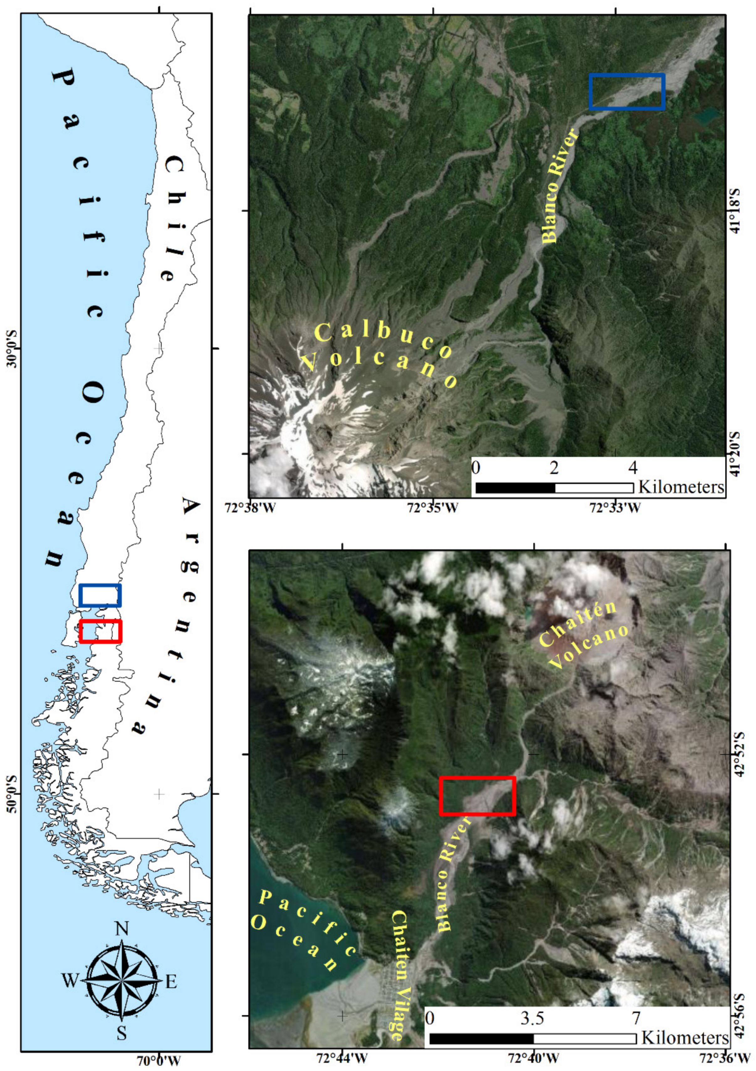
2.1. Study Area

The study was carried out in two reaches of two mountain rivers in southern Chile (Figure 1), both severely affected by volcanic eruptions; the Blanco River (hereinafter BR) (Chaitén), and the Blanco Este River (hereinafter BER) (Puerto Varas).

The BR is located 254 km south of Puerto Montt in southern Chile. This river was severely affected by the 2008 eruption of the Chaitén volcano. It is consistently sourced by LW from active channel lateral migration to destroyed riparian forest remnants and exhumation of volcanic deposits. More complete descriptions of the processes triggered by the eruption and the associated effects on the riverbed and riparian forests of the Blanco River can be found in [16,36,37,38,39].

This study was carried out in the same reach already considered by [35] with a length of 120 m and an area of 1.2 ha (Figure 1). The channel flows in a steep curve, has a longitudinal slope of approximately 1.2%, and features a gravel bed (D₅₀ = 26.2 mm) with patches of fine material (i.e., lithic rhyolite sand), provided mainly by the erosion of volcanic deposits. The riparian vegetation corresponds to the type of evergreen forest described by [40], and the predominant species in the fluvial corridor are Nothofagus dombeyi, N. betuloides, Drimys winteri, and several Myrtaceae, which were severely affected by the eruption of the Chaitén volcano in 2008 [38].

BER is a fluvial system located 40 km NE of Puerto Montt in southern Chile. This river was severely affected by the eruption of the Calbuco volcano in 2015. The channel flows in a SW-NW direction from its source on the eastern side of the Calbuco Volcano to its mouth at the confluence with the Petrohué River with an approximate length of 17.4 km. The specific study site reach is 220 m long, with an average width of 213 m, a total area of 4.6 ha (Figure 1), with a longitudinal slope of approximately 3.4% and a gravel bed (D₅₀ = 67 mm). The riparian vegetation corresponds to an evergreen native forest cover with patches of forest plantations.

2.2. Field Surveys

Field surveys were carried out to measure jam forming logs (hereinafter JFLW) within the study area to be able to check the precision of the proposed methodology. This step contains two tasks: (1) field surveys to accurately identify and georeference JFLW, measuring the diameter and length of each of them.

The WJs were georeferenced using a Trimble^® R6 dGPS with average horizontal and vertical precisions of 2 and 4 cm, respectively. Each WJ was georeferenced at the top and center of the accumulation. Following [41], the diameter and length of each JFLW, were measured with a caliper (estimated precision ≤1 cm) and tape (estimated precision ≤5 cm), respectively. The volume of each accumulation was calculated by summing the volumes of each of the individual logs, which were obtained using the formula for calculating the volume of a cylinder, following [35]:

V = π (D/2)² L

(1)

where V is the volume of each JFLW (m³), D is the diameter (m), and L is the length (m).

(2) UAV surveys (performed simultaneously to JFLW measurements) to obtain high resolution RGB images. Specifically, in the BR study area, 58 ground control points were set and georeferenced with a Trimble ^® R6 dGPS. A flight 50 m above the ground was carried out using a DJI S900 hexacopter, equipped with a 20-megapixel Nikon Coolpix A camera. Instead, in the BER study area, four flights were made 70 m above the ground with a DJI Phantom 4 Pro quadcopter, equipped with a 20 mega pixels stock camera. Here, 48 ground control points were set and georeferenced using the same Trimble^® R6 dGPS.

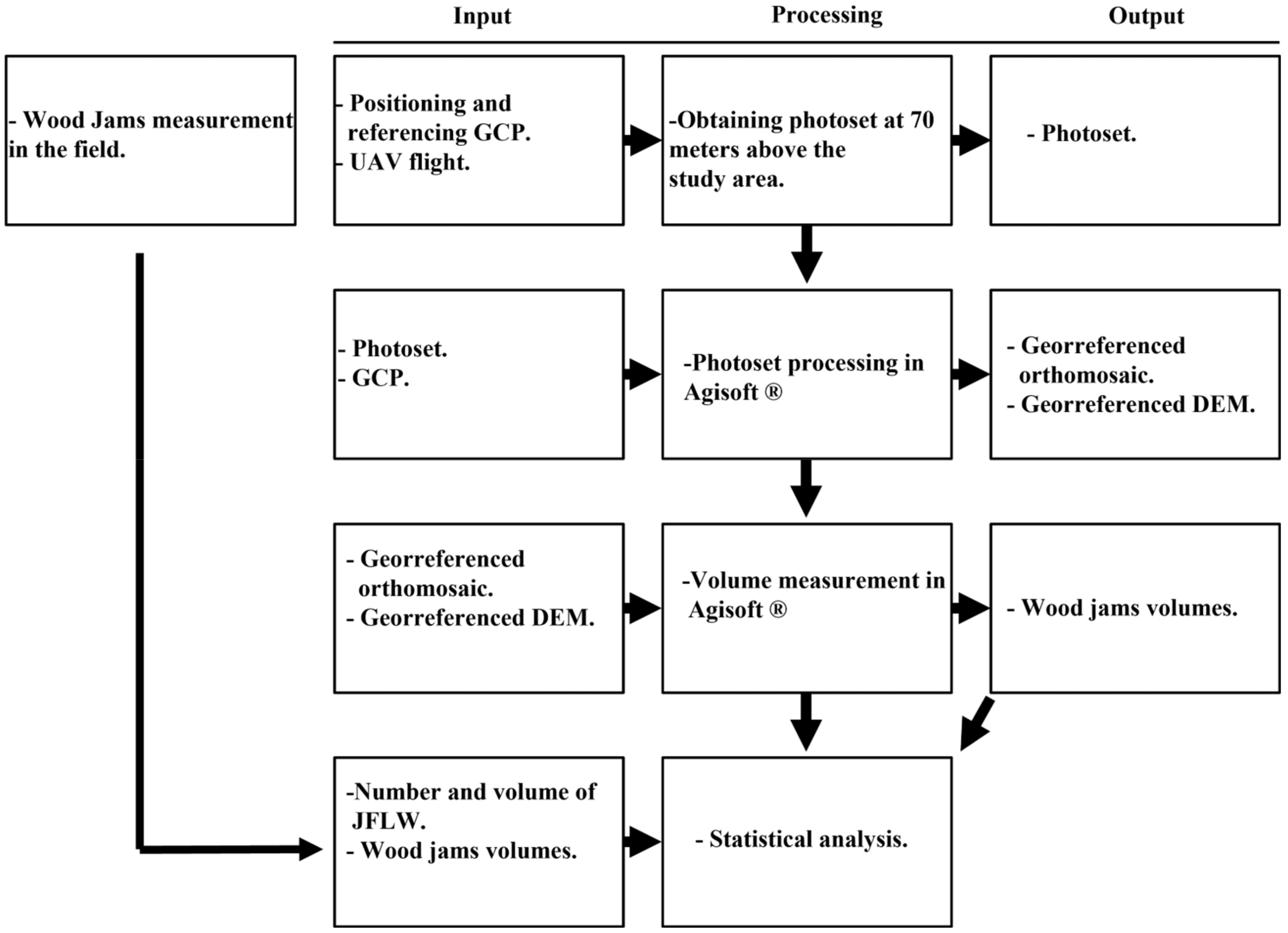
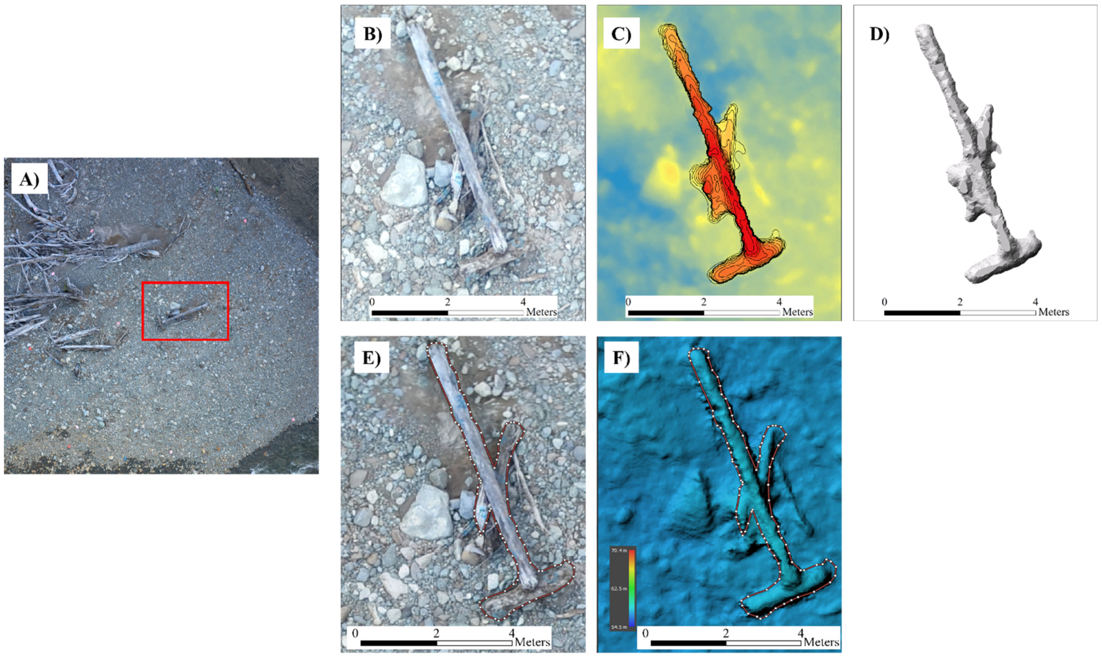
2.3. Arcgis Approach

The approach proposed in [35] (hereinafter ArcGIS approach) was implemented with ArcGIS ^®. The orthomosaic was used first to detect the WJs, and the DEM was used second to extract contour lines and generate a vector representation of the surface using Terrain Irregular Networks (TIN) through the “nearest neighbours” interpolation method from which the volume of the WJs was computed.

2.4. Agisoft Approach

On the contrary, in the new approach (hereinafter Agisoft approach), the RGB images were subsequently processed using Agisoft Metashape^® software (Agisoft Metashape Professional, Version: 1.5.5 build 9097 (64 bit), Owner: 2019 © AgiSoft LLC’s: 11B Degtyarnyi per., St. Petersburg, Russia, 191144) to generate a georeferenced orthomosaic (pixel dimension of 2.1 cm). In addition, a point cloud was produced to create the DEM of the study area (resulting by default from processing in maximum resolution cells of 2.2 cm).

The orthomosaic workspace was selected in AgiSoft^® and the wood accumulations were located on it, and the contours of each accumulation were drawn. Subsequently, the workspace of the DEM was selected, keeping the polygons of the drawn contours on which the “measure volume” tool was used.

Finally, analyses were carried out to determine if there were statistically significant differences between the data collected from the field and those measured digitally using the non-parametric tests Kruskal–Wallis (KW) (significance level of 95%) and Mann–Whitney (MW) (significance level of 95%), with which statistical tests were performed both to the total volumes of the accumulations (WJ) and to the individual logs of each accumulation (JFLW).

A graphical summary (Figure 2) of the workflow of the new approach shows the work methodology, while Figure 3 shows the different steps for identifying, delineating, and measuring the volume of a wood jam applying the Arcgis and Agisoft approaches.

2.5. Measurement Time Recording

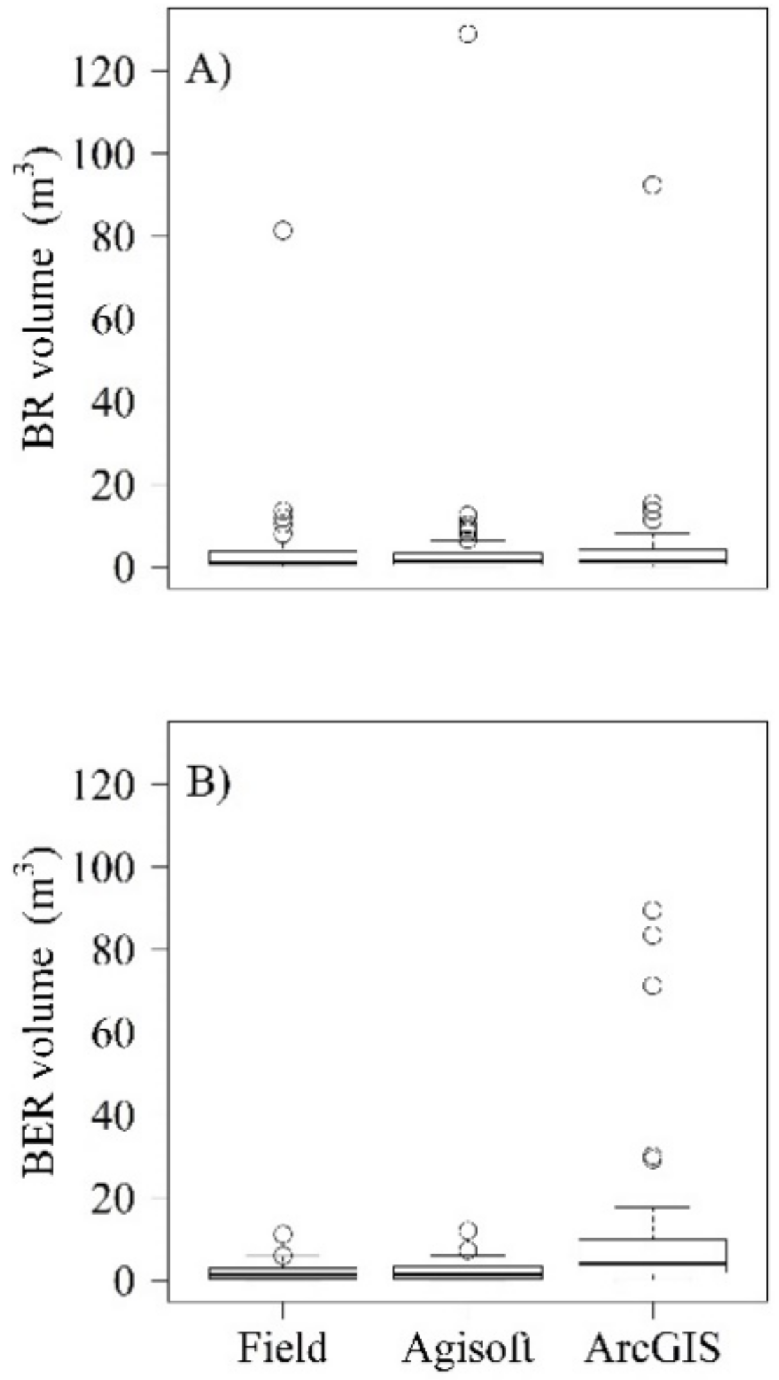
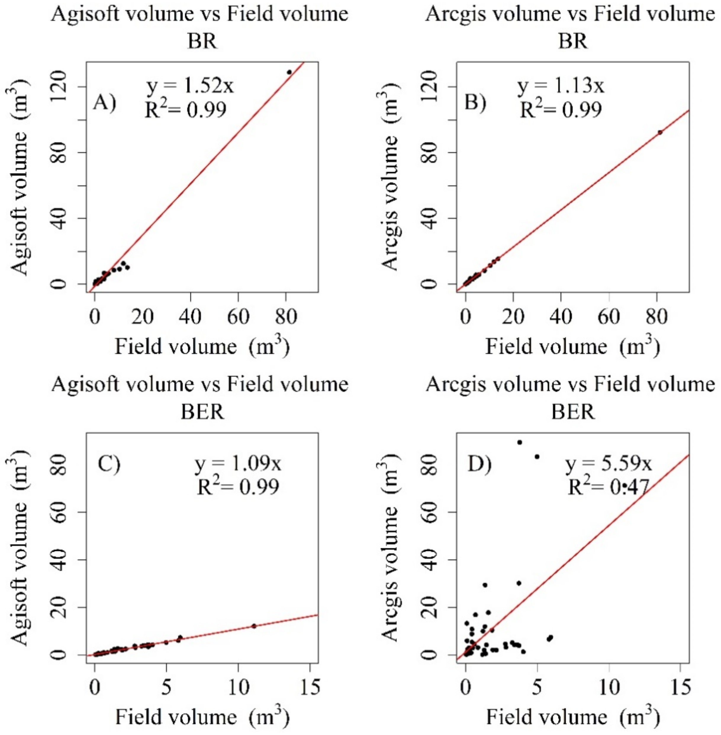
Moreover, analysis of the laboratory activity time was carried out for both study areas. The post-processing time was calculated for both methodologies to estimate eventual differences in the duration of both approaches to obtain the same results.

3. Results

Contrary to what was analyzed in [35], in this study only the WJs were considered since the methodological improvements are related just to these woody typologies. Considering this, in the next section the characterization of JFLW and WJ is presented.

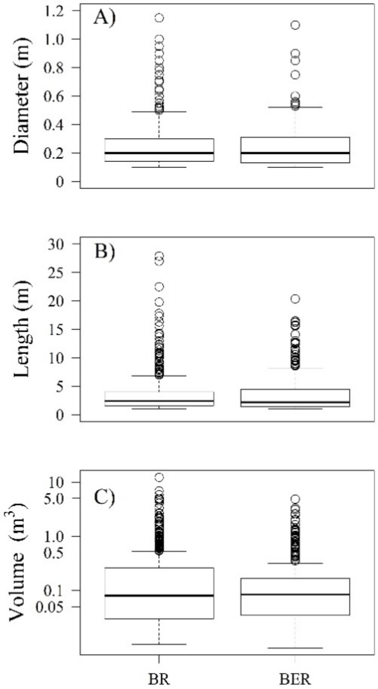
3.1. Field Surveys, Arcgis Approach and Agisoft Approach

All the wood jams located into the study reaches were considered. In BR, 37 WJs were detected and measured. These WJ were composed of 522 JFLWs, as already presented in [35]. On the other hand, along the BER, 45 WJ were found, composed of 382 JFLW that were measured in the field. Considering both datasets (i.e., BR and BER), differences in the diameter (

Table 1. Statistical summaries of (A) the diameters, lengths, and volumes of each JFLW measured manually in the field and (B) total volumes of WJ obtained with each method: Field Volume, Agisoft and Arcgis approaches. Q1 and Q3 correspond to the first and third quartile, respectively.

(A)	BR	BER	(B)	BR	BER
Diameter (m) Minimum Q1 Median Mean Q3 Maximum IQR	0.10 0.14 0.20 0.25 0.30 1.15 0.16	0.10 0.13 0.20 0.24 0.31 1.10 0.18	Field Volume (m3) Minimum Q1 Median Mean Q3 Maximum IQR	0.06 0.47 0.98 4.69 3.81 81.41 3.34	0.04 0.31 1.21 1.81 2.82 11.10 2.51
Length (m) Minimum Q1 Median Mean Q3 Maximum IQR	1.00 1.60 2.40 3.48 4.00 27.90 2.40	0.10 0.13 0.20 0.24 0.31 1.10 0.18	Agisoft Volume (m3) Minimum Q1 Median Mean Q3 Maximum IQR	0.05 0.59 1.57 6.15 3.30 129 2.71	0.06 0.40 1.48 2.06 3.35 11.99 2.95
Volume (m3) Minimum Q1 Median Mean Q3 Maximum IQR	0.01 0.03 0.08 0.34 0.26 12.25 0.23	0.01 0.03 0.08 0.22 0.17 4.84 0.13	Arcgis Volume (m3) Minimum Q1 Median Mean Q3 Maximum IQR	0.06 0.57 1.29 5.31 4.14 92.38 3.57	0.09 1.84 4.14 10.89 9.91 89.52 8.07

A; Figure 4A), length (Table 1A; Figure 4B), and volume (Table 1; Figure 4C) of each JFLW were not statistically significant (MW test), with p-values = 0.41, 0.10, and 0.58, respectively.

In BR, the biggest JFLW was characterized by a diameter of 1.15 m, a length of 27.90 m, and a volume of 12.25 m³ (Table 1A). On the contrary, along the BER, smaller JFLW were detected. Despite the maximum diameter being just slightly smaller than in BR (1.10 m), bigger differences are reported for length and volume, with maximum values equal to 20.30 m and 4.84 m³, respectively (Table 1A).

The WJ volumes in BR (Table 1B; Figure 5A) are not significantly different (KW test, p-value = 0.80), while for the BER (Table 1B; Figure 5B;) there are significant differences (KW test, p-value < 0.01) among the results obtained applying the different methodologies.

Considering the Blanco River, both methodological approaches appear highly accurate, showing a statistically significant linear correlation (MW test < 5%) (Figure 5). As already seen in [35], an overestimation of the field results was also detected with the Agisoft approach. For this specific study case, the wood volume allocated in WJs is overestimated by approximately 31.16 % in respect of those obtained by field measurements (227.42 m³ and 173.39 m³, respectively), contrary to the 13.3% obtained in [35].

Considering then the BER, interesting differences appeared using the different approaches (Figure 6). In fact, clear differences in performance can be ascribed to the different approach applied for WJ volume computation. The Agisoft approach also shows in this case a statistically significant linear correlation (MW test < 5%), generating an overestimation of approximately 12.3% with respect to field observation. On the contrary, the application of the ArcGIS approach does not work precisely even if maintaining a positive correlation. In this case, there is an overestimation of approximately 446.73%, with respect to field results.

3.2. Measurement Time Recording

Considering then the software processing time, in BR (

Table 2. Shows the summary of software processing times in both study areas and using the two methodologies.

	Measurement Time
	BR		BER
	Arcgis	Agisoft	Arcgis	Agisoft
	hh:mm:ss	hh:mm:ss	hh:mm:ss	hh:mm:ss
Total	04:34:43	00:44:51	04:23:05	00:45:06
Mean	00:07:25	00:01:13	00:05:51	00:01:00
Maximum	00:45:21	00:13:00	00:13:29	00:06:00
Minimum	00:03:26	00:00:20	00:03:44	00:00:20

) using the ArcGIS approach it was 6.1 times slower than the AgiSoft approach (total of 4 h 34 min vs. 45 min). Moreover, the AgiSoft approach was 3.5 times faster than the ArcGIS approach in the longest WJ measurement (13 min vs. 45 min) and 10.3 times faster in the shortest WJ measurement (20 s vs. 3 min 26 s).

In BER, the total software processing time with the ArcGIS approach was 5.8 times slower than the AgiSoft approach (4 h 23 min vs. 45 min). The AgiSoft approach was 2.2 times faster than the ArcGIS approach in the shortest WJ measurement (6 min vs. 13 min) and 11.2 times faster in the longest WJ measurement (20 s vs. 3 min 44 s).

4. Discussion

Based on the presented results, there were differences in the accuracy of both approaches (i.e., ArcGIS and Agisoft) for estimating the volume of WJs. As already seen in [35] and with the Agisoft approach, there is still overestimation for both study cases (i.e., 31.16 % and 12.30% for BR and BER, respectively). Porosity has already been recognized as a determining factor in the overestimation of the WJ volume [12], and it can also be responsible for these approaches. For instance, Ref. [42] determined the proportion of air between 18.9% and 93% in WJs from two rivers in south-eastern France, and [43] studied WJs along a stretch of the Highland Water in southern England with high degrees of porosity (80%). The precision of UAV methodology varies depending on the composition of the WJ (i.e., quantity and characteristics of JFLW, their mutual orientation, and the shape of WJ) and the morphological setting of the channel (i.e., complexity, slope, grainsize). Therefore, differences in the results of both approaches in this research can be explained by three main factors: (i) different computational methods for calculating the volumes; (ii) differences between the bed grain sizes; and iii) differences between the wood dimensions in both study areas. An important factor is the interpolation methods used by each approach to represent the form of the WJs. The ArcGIS approach uses “Nearest Neighbors” to create a TIN and to represent the form of the WJs, while the AgiSoft^® interpolation method is IDW. This could be a determining factor since there are interpolation methods that are more accurate than others to represent surfaces [44,45].

Differences in grain size are important since they determine the roughness of the surface where the LW is deposited and also the porosity. In BR (D50 = 26.2 mm), there is a smoother, less rough surface, while in BER (D50 = 67 mm) there is a rougher surface. Porosity is an important problem when determining the volume of the LW [12] because air spaces generate overestimation [42].

The ArcGIS approach works better (is more precise) in BR (13.2% difference with respect to the volume measured in the field, versus a 31.1% difference obtained with the Agisoft approach), and this can be ascribable to the fact that the wood is thicker [46] and the ground is smoothed, favouring the delineation of each JFLW and reducing the inclusion of porosity in the computation; in contrast, the approach proposed in this study is more precise in BER, where the wood is thinner, and the channel surface is rougher [47]. The Agisoft approach works better (is more precise) in BER (12.3% difference with respect to the volume measured in the field, compared to a difference of 494.8% overestimation obtained by the ArcGIS approach). This is probably due to the presence of such bigger boulders and cobbles that permit better digitalization of the JFLW (maintaining it suspended over the ground) defining the volumes in a more precise way and avoiding the computation of porosity as wood volume. This may suggest that this new approach fits better with such characteristics in JFLW and roughness (i.e., small logs and big cobbles), while the original approach proposed apparently fits better with rivers having bigger JFLW and finer substrate.

However, in terms of processing time, the Agisoft approach works much faster, using a single software to perform all post-processing, from photo set processing to volume measurements. Due to the reduced number of steps, the Agisoft approach is approximately six times faster in terms of post-processing time. This new approach can be applied to quantify the volume of wood after extreme events, such as lahars, which can considerably increase the sediment load and debris flow processes in river courses after volcanic eruptions [48].This approach, as well as that of ArcGIS, is less risky for field operators since the field work is limited to UAV flights and GCP measurement, reducing a lot time spent in the field, where sudden movements can be risky for operators doing traditional measurements (i.e., using tape and tree callipers) and permitting continuation with research subsequent to extreme events, such as those of the Blanco River after the eruption of the Chaitén volcano [49] and the Blanco Este River after the Calbuco volcano eruption [50], which can be more safely studied in the field.

5. Conclusions

Remote sensing analyses can estimate the volume of LW in riverbeds, saving large amounts of time and resources, reducing working time in the field and in post-process operations and thus optimizing economic resources. In addition, working from a remote perspective reduces the risks of working in unstable environments by reducing exposure to risk factors present in rivers, such as sudden movements of soil, water, or sediment. The Agisoft approach presented in this research, accomplished objectives well with a combination of adequate precision and reduction of working time. These results can be further improved through automatization of the process of LW individuation and detection. This last step would greatly improve the detection of WJ, minimizing both operator errors and the time consumption of the operator at the desk.

References

1. Jackson, C.R.; Sturm, C.A. Woody Debris and Channel Morphology in First- and Second-Order Forested Channels in Washington’s Coast Ranges. Water Resour. Res. 2002, 38, 16-1–16-14. [Google Scholar] [CrossRef] [Green Version]
2. Gurnell, A.M.; Pié Gay, H.; Swanson, F.J.; Gregory, S.V. Large Wood and Fluvial Processes. Freshw. Biol. 2002, 47, 601–619. [Google Scholar] [CrossRef] [Green Version]
3. Spreitzer, G.; Tunnicliffe, J.; Friedrich, H. Using Structure from Motion Photogrammetry to Assess Large Wood (LW) Accumulations in the Field. Geomorphology 2019, 346, 106851. [Google Scholar] [CrossRef]
4. Picco, L.; Scalari, C.; Iroumé, A.; Mazzorana, B.; Andreoli, A. Large Wood Load Fluctuations in an Andean Basin. Earth Surf. Process. Landf. 2021, 46, 371–384. [Google Scholar] [CrossRef]
5. Mazzorana, B.; Picco, L.; Rainato, R.; Iroumé, A.; Ruiz-Villanueva, V.; Rojas, C.; Valdebenito, G.; Iribarren-Anacona, P.; Melnick, D. Cascading Processes in a Changing Environment: Disturbances on Fluvial Ecosystems in Chile and Implications for Hazard and Risk Management. Sci. Total Environ. 2019, 655, 1089–1103. [Google Scholar] [CrossRef]
6. Piégay, H.; Thévenet, A.; Citteio, A. Input, Storage and Distribution of Large Woody. Catena 1999, 35, 19–39. [Google Scholar] [CrossRef]
7. Gurnell, A.M.; Petts, G.E.; Hannah, D.M.; Smith, B.P.G.; Edwards, P.J.; Kollmann, J.; Ward, J.V.; Tockner, K. Wood Storage within the Active Zone of a Large European Gravel-Bed River. Geomorphology 2000, 34, 55–72. [Google Scholar] [CrossRef]
8. Andreoli, A.; Comiti, F.; Lenzi, M.A. Characteristics, Distribution and Geomorphic Role of Large Woody Debris in a Mountain Stream of the Chilean Andes. Earth Surf. Process. Landf. 2007, 32, 1675–1692. [Google Scholar] [CrossRef]
9. Wohl, E.; Cadol, D. Neighborhood Matters: Patterns and Controls on Wood Distribution in Old-Growth Forest Streams of the Colorado Front Range, USA. Geomorphology 2011, 125, 132–146. [Google Scholar] [CrossRef]
10. Wohl, E.; Lininger, K.B.; Fox, M.; Baillie, B.R.; Erskine, W.D. Instream Large Wood Loads across Bioclimatic Regions. Ecol. Manag. 2017, 404, 370–380. [Google Scholar] [CrossRef]
11. Ulloa, H.; Iroumé, A.; Picco, L.; Korup, O.; Lenzi, M.A.; Mao, L.; Ravazzolo, D. Massive Biomass Flushing despite Modest Channel Response in the Rayas River Following the 2008 Eruption of Chaitén Volcano, Chile. Geomorphology 2015, 250, 397–406. [Google Scholar] [CrossRef]
12. Livers, B.; Lininger, K.B.; Kramer, N.; Sendrowski, A. Porosity Problems: Comparing and Reviewing Methods for Estimating Porosity and Volume of Wood Jams in the Field. Earth Surf. Process. Landf. 2020, 45, 3336–3353. [Google Scholar] [CrossRef]
13. Marcus, W.A.; Marston, R.A.; Colvard, C.R.C.; Gray, R.D. Mapping the Spatial and Temporal Distributions of Woody Debris in Streams of the Greater Yellowstone Ecosystem, USA. Geomorphology 2002, 44, 323–335. [Google Scholar] [CrossRef] [Green Version]
14. Marcus, W.A.; Legleiter, C.J.; Aspinall, R.J.; Boardman, J.W.; Crabtree, R.L. High Spatial Resolution Hyperspectral Mapping of In-Stream Habitats, Depths, and Woody Debris in Mountain Streams. Geomorphology 2003, 55, 363–380. [Google Scholar] [CrossRef]
15. Atha, J.B. Identification of Fluvial Wood Using Google Earth. River Res. Appl. 2014, 30, 857–864. [Google Scholar] [CrossRef]
16. Ulloa, H.; Iroumé, A.; Mao, L.; Andreoli, A.; Diez, S.; Lara, L.E. Use of Remote Imagery to Analyse Changes in Morphology and Longitudinal Large Wood Distribution in the Blanco River After the 2008 Chaitén Volcanic Eruption, Southern Chile. Geogr. Ann. Ser. A Phys. Geogr. 2015, 97, 523–541. [Google Scholar] [CrossRef]
17. Kasprak, A.; Magilligan, F.J.; Nislow, K.H.; Snyder, N.P. A Lidar-Derived Evaluation of Watershed-Scale Large Woody Debris Sources and Recruitment Mechanisms: Coastal Maine, USA. River Res. Appl. 2012, 28, 1462–1476. [Google Scholar] [CrossRef] [Green Version]
18. Gonzalez de Tanago, J.; Lau, A.; Bartholomeus, H.; Herold, M.; Avitabile, V.; Raumonen, P.; Martius, C.; Goodman, R.C.; Disney, M.; Manuri, S.; et al. Estimation of Above-Ground Biomass of Large Tropical Trees with Terrestrial LiDAR. Methods Ecol. Evol. 2018, 9, 223–234. [Google Scholar] [CrossRef] [Green Version]
19. Boivin, M.; Bélanger, B. Using a Terrestrial LIDAR for Monitoring of Large Woody Debris Jams in Gravel Bed Rivers. In Proceedings of the 7th Gravel Bed Rivers Conference, Tadoussac, QC, Canada, 5–10 September 2010. [Google Scholar]
20. Tonon, A.; Picco, L.; Ravazzolo, D.; Lenzi, M.A. Using a Terrestrial Laser Scanner to Detect Wood Characteristics in Gravel-Bed Rivers. J. Agric. Eng. 2014, 45, 161–167. [Google Scholar] [CrossRef] [Green Version]
21. Grigillo, D.; Gvozdanović, M.; Anžur, T.; Vezočnik, A. Determination of Large Wood Accumulation in a Steep Forested Torrent Using Laser Scanning. Eng. Geol. Soc. Territ. 2015, 3, 127–130. [Google Scholar]
22. Entwistle, N.; Heritage, G.; Milan, D. Recent Remote Sensing Applications for Hydro and Morphodynamic Monitoring and Modelling. Earth Surf. Process. Landf. 2018, 43, 2283–2291. [Google Scholar] [CrossRef]
23. Hackney, C.; Clayton, A. Unmanned Aerial Vehicles (UAVs) and Their Application in Geomorphic Mapping. In Geomorphological Techniques; British Society for Geomorphology: London, UK, 2015. [Google Scholar]
24. Tamminga, A.D.; Eaton, B.C.; Hugenholtz, C.H. UAS-Based Remote Sensing of Fluvial Change Following an Extreme Flood Event. Earth Surf. Process. Landf. 2015, 40, 1464–1476. [Google Scholar] [CrossRef]
25. Turner, D.; Lucieer, A.; Watson, C. An Automated Technique for Generating Georectified Mosaics from Ultra-High Resolution Unmanned Aerial Vehicle (UAV) Imagery, Based on Structure from Motion (SFM) Point Clouds. Remote Sens. 2012, 4, 1392–1410. [Google Scholar] [CrossRef] [Green Version]
26. Turner, D.; Lucieer, A.; Malenovský, Z.; King, D.H.; Robinson, S.A. Spatial Co-Registration of Ultra-High Resolution Visible, Multispectral and Thermal Images Acquired with a Micro-UAV over Antarctic Moss Beds. Remote Sens. 2014, 6, 4003–4024. [Google Scholar] [CrossRef] [Green Version]
27. Woodget, A.S.; Fyffe, C.; Carbonneau, P.E. From Manned to Unmanned Aircraft: Adapting Airborne Particle Size Mapping Methodologies to the Characteristics of SUAS and SfM. Earth Surf. Process. Landf. 2018, 43, 857–870. [Google Scholar] [CrossRef]
28. Javernick, L.; Brasington, J.; Caruso, B. Modeling the Topography of Shallow Braided Rivers Using Structure-from-Motion Photogrammetry. Geomorphology 2014, 213, 166–182. [Google Scholar] [CrossRef]
29. Lucieer, A.; de Jong, S.M.; Turner, D. Mapping Landslide Displacements Using Structure from Motion (SfM) and Image Correlation of Multi-Temporal UAV Photography. Prog. Phys. Geogr. 2014, 38, 97–116. [Google Scholar] [CrossRef]
30. Smith, M.W.; Vericat, D. From Experimental Plots to Experimental Landscapes: Topography, Erosion and Deposition in Sub-Humid Badlands from Structure-from-Motion Photogrammetry. Earth Surf. Process. Landf. 2015, 40, 1656–1671. [Google Scholar] [CrossRef] [Green Version]
31. Llena, M.; Vericat, D.; Martínez-Casasnovas, J.A. Application of Structure from Motion (SfM) Algorithms for the Historical Analysis of Changes in Fluvial Geomorphology. Cuatern. Geomorfol. 2018, 32, 53–73. [Google Scholar] [CrossRef] [Green Version]
32. Woodget, A.S.; Austrums, R. Subaerial Gravel Size Measurement Using Topographic Data Derived from a UAV-SfM Approach. Earth Surf. Process. Landf. 2017, 42, 1434–1443. [Google Scholar] [CrossRef]
33. Bakker, M.; Lane, S.N. Archival Photogrammetric Analysis of River–Floodplain Systems Using Structure from Motion (SfM) Methods. Earth Surf. Process. Landf. 2017, 42, 1274–1286. [Google Scholar] [CrossRef] [Green Version]
34. Truksa, T.; Browman, J.; Goodge, J. Can Drones Measure LWD High Resolution Aerial Imagery and Structure from Motion as a Method for Quantifying Instream Wood. In Proceedings of the GSA Annual Meeting, Seattle, WA, USA, 22–25 October 2017; p. 12. [Google Scholar]
35. Sanhueza, D.; Picco, L.; Ruiz-Villanueva, V.; Iroumé, A.; Ulloa, H.; Barrientos, G. Quantification of Fluvial Wood Using UAVs and Structure from Motion. Geomorphology 2019, 345, 106837. [Google Scholar] [CrossRef]
36. Major, J.J.; Pierson, T.C.; Hoblitt, R.P.; Moreno, H. Flujos Piroclásticos Asociados a La Erupción 2008-2009 Del Volcán Chaitén: Perturbación Del Bosque, Depósitos y Dinámica. Andean Geol. 2013, 40, 324–358. [Google Scholar] [CrossRef] [Green Version]
37. Major, J.J.; Bertin, D.; Pierson, T.C.; Amigo, Á.; Iroumé, A.; Ulloa, H.; Castro, J. Extraordinary Sediment Delivery and Rapid Geomorphic Response Following the 2008–2009 Eruption of Chaitén Volcano, Chile. Water Resour. Res. 2016, 52, 5075–5094. [Google Scholar] [CrossRef]
38. Swanson, F.J.; Jones, J.A.; Crisafulli, C.M.; Lara, A. Efectos de Los Procesos Volcánicos e Hidrológicos Sobre La Vegetación Forestal: El Volcán Chaitén, Chile. Andean Geol. 2013, 40, 359–391. [Google Scholar] [CrossRef] [Green Version]
39. Martini, L.; Picco, L.; Iroumé, A.; Cavalli, M. Sediment Connectivity Changes in an Andean Catchment Affected by Volcanic Eruption. Sci. Total Environ. 2019, 692, 1209–1222. [Google Scholar] [CrossRef]
40. Donoso, Z. Claudio Reseña Ecológica de Los Bosques Mediterráneos de Chile. Bosque 1982, 4, 117–146. [Google Scholar] [CrossRef]
41. Iroumé, A.; Andreoli, A.; Comiti, F.; Ulloa, H.; Huber, A. Large Wood Abundance, Distribution and Mobilization in a Third Order Coastal Mountain Range River System, Southern Chile. Ecol. Manag. 2010, 260, 480–490. [Google Scholar] [CrossRef]
42. Thevenet, A.; Citterio, A.; Piegay, A.H. A New Methodology for the Assessment of Large Woddy Debris Accumulations on Highly Modified Rivers (Example of Two French Piedmont Rivers). Regul. Rivers Res. Manag. Int. J. Dev. River Res. Manag. 1998, 14, 467–483. [Google Scholar] [CrossRef]
43. Dixon, S.J. A Dimensionless Statistical Analysis of Logjam Form and Process. Ecohydrology 2016, 9, 1117–1129. [Google Scholar] [CrossRef] [Green Version]
44. Heritage, G.L.; Milan, D.J.; Large, A.R.G.; Fuller, I.C. Influence of Survey Strategy and Interpolation Model on DEM Quality. Geomorphology 2009, 112, 334–344. [Google Scholar] [CrossRef]
45. Arun, P.V. A Comparative Analysis of Different DEM Interpolation Methods. Egypt. J. Remote Sens. Space Sci. 2013, 16, 133–139. [Google Scholar]
46. Tonon, A.; Iroumé, A.; Picco, L.; Oss-Cazzador, D.; Lenzi, M.A. Temporal Variations of Large Wood Abundance and Mobility in the Blanco River Affected by the Chaitén Volcanic Eruption, Southern Chile. Catena 2017, 156, 149–160. [Google Scholar] [CrossRef]
47. Kreuzbug, F. Ganulometría y Competencia El Río Blanco Este (Sur de Chile). Impactado Por La Erupción Del Volcán Calbuco En 2015. Ph.D. Thesis, Universidad Austral de Chile, Valdivia, Chile, 2019. [Google Scholar]
48. Smith, G. Facies Sequences and Geometries in Continental Volcaniclastic Sediments. In Sedimentation in Volcanic Settings; Society for Sedimentary Geology: Tulsa, OK, USA, 1991. [Google Scholar]
49. Iroumé, A.; Paredes, A.; Garbarino, M.; Morresi, D.; Batalla, R.J. Post-Eruption Morphological Evolution and Vegetation Dynamics of the Blanco River, Southern Chile. J. South Am. Earth Sci. 2020, 104, 102809. [Google Scholar] [CrossRef]
50. Mixon, E.E.; Singer, B.S.; Jicha, B.R.; Ramirez, A. Calbuco, a Monotonous Andesitic High-Flux Volcano in the Southern Andes, Chile. J. Volcanol. Geotherm. Res. 2021, 416, 107279. [Google Scholar] [CrossRef]
Figure 1. Study area locations in Chile (left), and the specific location of Blanco Este River (top-right) and Blanco River (bottom right) (modified after [35]).
Drones 06 00218 g001
Figure 2. Workflow detailing each stage of the methodological process, the necessary input, the processing, and their outputs. Keywords: GCP (ground control points), UAV (unmanned aerial vehicle), Photoset (set of images obtained from the UAV flight), DEM (digital elevation model), Orthomosaic (mosaic built from the photoset), JFLW (jams forming logs) (modified after [35]).
Drones 06 00218 g002
Figure 3. Different steps to follow for the digital measurement process, starting from (A) the individuation of a WJ in the red frame, (B) shows the WJ on the mosaic obtained from the photoset using Arcgis, (C) shows the WJ delimited and with contour lines on the DEM, in Arcgis, (D) shows the generated TIN in Arcgis that permit the calculation of the wood volume, (E) shows the WJ delimited with a polygon on the mosaic obtained from the photos in Agisoft, (F) shows the polygon on the DEM (hillshade effect) from which the wood volume is calculated in Agisoft.
Drones 06 00218 g003
Figure 4. Boxplots of JFLW diameter (A), length (B), and volume (C) for the Blanco River (BR) (n = 522) and Blanco Este River (BER) (n = 382). The bottom and top of the box indicate the first and the third quartiles, respectively, the line inside the box is the median value, the whiskers are the highest values within 1.5 interquartile range from the third quartile and a minimum value, whereas circles are the outliers and the extreme values, respectively.
Drones 06 00218 g004
Figure 5. Boxplots of WJ volumes detected using three different approaches along the Blanco River (BR) (n = 37) (A), and the Blanco Este River (BER) (n = 45) (B). Boxplots as in Figure 3.
Drones 06 00218 g005
Figure 6. Relationships between the volumes of WJ obtained from the field versus those obtained from digital analysis methodologies, using Agisoft (A,C) and Arcgis (B,D) in BR (A,B) and BER (C,D), respectively.
Drones 06 00218 g006