Article

Research on Scenario Modeling for V-Tail Fixed-Wing UAV Dynamic Obstacle Avoidance

1
School of Intelligent Systems Engineering, Sun Yat-sen University, Shenzhen 518107, China
2
Southern Marine Science and Engineering Guangdong Laboratory (Zhuhai), Zhuhai 519000, China
3
School of Civil Aviation, Northwestern Polytechnical University, Xi’an 710072, China
4
Unmanned Aerial System Co., Ltd., Aviation Industry Corporation of China (Chengdu), Chengdu 610091, China
*
Author to whom correspondence should be addressed.
Drones 2023, 7(10), 601; https://doi.org/10.3390/drones7100601
Submission received: 8 August 2023 / Revised: 11 September 2023 / Accepted: 21 September 2023 / Published: 25 September 2023

Abstract

:
With the advantages of long-range flight and high payload capacity, large fixed-wing UAVs are often used in anti-terrorism missions, disaster surveillance, and emergency supply delivery. In the existing research, there is little research on the 3D model design of the V-tail fixed-wing UAV and 3D flight environment modeling. The study focuses on designing a comprehensive simulation environment using Gazebo and ROS, referencing existing large fixed-wing UAVs, to design a V-tail aircraft, incorporating realistic aircraft dynamics, aerodynamics, and flight controls. Additionally, we present a simulation environment modeling approach tailored for obstacle avoidance in no-fly zones, and have created a 3D flight environment in Gazebo, generating a large-scale terrain map based on the original grayscale heightmap. This terrain map is used to simulate potential mountainous terrain threats that a fixed-wing UAV might encounter during mission execution. We have also introduced wind disturbances and other specific no-fly zones. We integrated the V-tail fixed-wing aircraft model into the 3D flight environment in Gazebo and designed PID controllers to stabilize the aircraft’s flight attitude.

1. Introduction

A V-tail aircraft is a distinct class of aircraft that features a V-shaped tail configuration. This unconventional design replaces the traditional horizontal stabilizer and vertical fin with two surfaces angled to form a V shape, which serve as both elevator and rudder control surfaces [1]. The V-tail design offers advantages such as reduced weight, improved maneuverability, and reduced drag [2]. Due to these advantages of the V-shaped tail, this tail design is widely used in large fixed-wing UAVs in various countries, such as the CAIG Wing Loong II, CASC Rainbow CH-4, and General Atomics MQ-9 Reaper [3].
The primary objective of this project is to create a realistic simulation framework using Gazebo and ROS for V-tail aircraft, allowing for the accurate modeling of their flight dynamics, control systems, and response to flight threat scenarios. Through leveraging the capabilities of Gazebo, a powerful physics-based simulator, and ROS, a flexible and widely used robotic framework [4,5,6,7], we can create a comprehensive and interactive simulation environment.
In existing research [8,9,10] on fixed-wing aircraft flight simulation, the majority of studies are based on developing flight dynamics models, control algorithms, and trajectory planning using MATLAB software. Scott et al. [11] developed a fixed-wing aircraft simulation tool that incorporates aerodynamics, structural dynamics, kinematics, and kinetics, but has only numerical simulation calculations and no visual scene interface. Deiler et al. [12] proposed dynamic aircraft simulation models that cover the effects of local icing, but did not incorporate actual flight scenarios, only numerical calculations. Heesbeen et al. [13] proposed a multi-purpose aircraft simulation architecture, but it requires a lot of hardware equipment. These studies [14,15,16,17,18] combined MATLAB and FlightGear for the flight simulation of aircraft. Horri et al. [19] studied the co-simulation of an aircraft using MATLAB combined with Xplane, FlightGear, and VFTE simulation software. These studies [20,21,22] combined MATLAB and X-Plane for co-simulation to design and verify the performance of aircraft controllers. There are also some aircraft simulation studies based on the Gazebo simulation platform. Yang et al. [23] studied the hardware-in-the-loop simulation of fixed-wing UAVs in Gazebo. Irmawan et al. [24] studied the 3D simulation of a VTOL fixed wing in Gazebo. Lee et al. [25,26] combined the PX4 autopilot and Gazebo simulation environment to test the controller performance of a fixed-wing aircraft under control surface failure conditions. Ellingson et al. [27] designed a fixed-wing autopilot for education and research and used Gazebo for the remote flight simulation of an aircraft model. In these simulation studies, most of them use existing aircraft models to simulate flight, and many of them do not combine the corresponding flight scenarios, and the scalability of the simulation platform is poor.
Different from the existing aircraft simulation framework, this paper focuses on the model establishment of V-tail aircraft and flight simulation based on Gazebo, and uses the powerful performance of the Gazebo simulator to create the flight threat scenario of aircraft and support the flight control of multiple aircraft in the same scenario. It lays a foundation for subsequent research on aircraft route planning algorithms and multi-aircraft cooperative flight algorithms. Through this project, we aim to provide researchers, engineers, and aviation enthusiasts with a robust and customizable simulation framework for V-tail aircraft, enabling them to evaluate the aircraft’s behavior under realistic conditions and explore novel flight threat scenarios. This simulation framework can serve as a valuable tool for performance analysis, algorithm development, and decision-making in V-tail aircraft-related research and development.
The paper is organized as follows. Section 2 introduces the simulation system framework used in this study. Section 3 provides the aerodynamics mathematical model of the fixed-wing aircraft and the establishment of the 3D model of the V-tail aircraft. Section 4 presents a simulation environment modeling approach tailored for obstacle avoidance in no-fly zones. Section 5 presents the attitude control of the V-tail aircraft in the Gazebo flight environment. Finally, Section 6 contains the conclusions.

2. Simulation System Framework

Gazebo and ROS are two powerful tools which are widely used in the field of robotics and simulation. Gazebo is an open-source, multi-robot simulator that provides a highly realistic and dynamic environment for simulating robots, UAVs, and complex systems. It allows for the simulation of physics-based interactions, sensor data, and control algorithms. ROS, on the other hand, is a flexible framework for building robotic systems. It provides a collection of software libraries, tools, and conventions that facilitate communication between different components of a robotic system. ROS enables the development of modular and scalable robotic applications through offering features such as message passing, service calls, and parameter management.
When combined, Gazebo and ROS form a powerful simulation environment that allows for the integration of realistic physics-based simulation with sophisticated robot control and interaction. This combination has become a standard in the robotics community for developing and testing robotic systems.
In the context of V-tail aircraft and flight threat scenario modeling, Gazebo provides a platform for creating a realistic simulation environment that accurately models the physics and dynamics of the aircraft. It enables the simulation of aerodynamic forces, environmental factors, and realistic sensor data. Gazebo’s visualization capabilities also allow for the real-time monitoring and visualization of the simulation.
Through leveraging the capabilities of Gazebo and ROS, researchers and engineers can create comprehensive and interactive simulations of V-tail aircraft and flight threat scenarios. This allows for the in-depth analysis of the aircraft’s behavior, performance evaluation, and the testing of control algorithms. The integration of Gazebo and ROS provides a seamless workflow, enabling users to develop and validate their models and algorithms in a realistic virtual environment before deploying them on real aircraft.

3. Fixed-Wing UAV Vehicle Modeling

3.1. Aircraft Aerodynamics

In the V-tail fixed-wing aircraft simulation environment created in this study, the primary reliance is on the aerodynamics plugin provided by Gazebo’s official sources to simulate the aircraft’s flight lift. Referring to existing literature [28,29,30], the following aerodynamics mathematical model is established.
Wind speed has a significant impact on UAV motion, which can have an impact on flight performance, flight trajectory, and control requirements. Taking the body coordinate system as a reference, the airspeed vector of the UAV is denoted as v r b , the ground speed vector is denoted as v b , and the wind speed vector is denoted as v ω b . Then, the relationship between wind speed, ground speed, and airspeed can be obtained as follows:
v r b = v b v ω b
The relationship between the size of UAV airspeed V a and the airspeed vector v r b of an UAV under the aircraft system is as follows:
v r b = ( u v w ) = R w b ( V a 0 0 ) = ( R b w ) T ( V a 0 0 ) = ( cos β cos   α sin β cos   α sin α sin β cos β 0 cos β sin α sin β sin α cos   α ) ( V a 0 0 )
where R w b is the rotation matrix from the air flow coordinate system to the body coordinate system, α is the angle of attack, β is the sideslip angle, and V a is the magnitude of the airspeed, which can be calculated using the following equation.
{ α = arctan ( w u ) β = arcsin ( v V a ) V a = u 2 + v 2 + w 2
The translational kinematic equation of the UAV is given by
p ˙ n = R b n v b
v r b = v b R n b v w i n d n
where p n represents the position of the UAV in the inertial frame, v b represents the ground velocity vector of the UAV in the aircraft system, R b n represents the rotation matrix from the aircraft system to the inertial frame, and v w i n d n represents the wind speed vector in the inertial frame.
The wind speed is assumed to be constant or slowly varying. Newton’s second law is applied to the UAV in translational motion, and the force and velocity under the UAV system are expressed as
d v r b d t b = S ( w n , b b ) v r b + f b m
where m is the mass of the UAV, d d t b is the time derivative in the body coordinate system, and f b is the sum of all external forces acting on the UAV under the aircraft system, including gravity, aerodynamic force, and thrust. w n , b b is the angular velocity between the machine system and the inertial frame.
f b = R n b f g n + R w b f a e r o w + f t h r u s t b
where f g n = [ 0   0   m g ] T is the heavy force vector under inertial system, and g is the acceleration degree of heavy force. f t h r u s t b = [ T   0   0 ] T is the thrust vector under the aircraft system. Most aircraft are designed with thrust directly along the aircraft body axis i b . f a e r o w is the aerodynamic force vector under the flow system, which can be expressed as
f a e r o w = 1 2 ρ S V a 2 [ ( C D 0 + k C L 2 ) C Y β β ( C L 0 + C L α α ) ]
where ρ is air density, S is the plane airfoil area, C ( · ) is the coefficient of aerodynamics, and C L = C L 0 + C L α α . k is a constant scalar value that depends on the aircraft configuration.
The quaternion based rotational kinematics equation of aircraft is as follows:
q ˙ n , b = 1 2 q n , b [ 0 ω n , b b ]
where q n , b represents the quaternion of rotation from the body coordinate system to the inertial system.
Under the body coordinate system, Euler’s momentum equation is applied to a rotating aircraft.
d h b d t b + ω n , b b × h b = τ a e r o b
where h b is the vector form of angular momentum under body coordinate system. τ a e r o b is the aerodynamic torque vector of body coordinate system. For a rigid body, angular momentum is defined as the product of the moment of inertia matrix J and the angular velocity vector: h b = J ω n , b b .
J = ( J x x J x y J x z J x y J y y J y z J x z J y z J z z )
Thus, Equation (10) can be rewritten as:
ω ˙ n , b b = J 1 [ S ( ω n , b b ) J ω n , b b + τ a e r o b ]
Aerodynamic torque is defined as:
τ a e r o b = f ( α , β ) D ω n , b n + B u
where u = [ δ a δ e δ r ] T is a vector consisting of three control quantities used to control the rotation angles of the aileron, elevator, and rudder. f ( α , β ) is the aerodynamic torque vector function, which can be expressed as:
f ( α , β ) = 1 2 ρ S V a 2 [ b ( C l 0 + C l β β ) c ¯ ( C m 0 + C m α α ) b ( C n 0 + C n β β ) ]
D is a positive definite matrix denoted by:
D = 1 2 ρ S V a 2 [ b 2 2 V a C l p 0 b 2 2 V a C l r 0 ( c ¯ ) 2 2 V a C m q 0 b 2 2 V a C n p 0 b 2 2 V a C n r ]
B is the control matrix and is defined as:
B = 1 2 ρ S V a 2 [ b C l δ a 0 b C l δ r 0 c ¯ C m δ e 0 b C n δ a 0 b C n δ a ]
where b is the wingspan length and c ¯ is the average aerodynamic chord.
In summary, the following dynamic model can be obtained through combining the translational motion and rotational motion of the fixed-wing aircraft.
{ p ˙ n = R b n v b v ˙ r b = S ( w n , b b ) v r b + ( R n b f g n + R w b f aero   w + f thrust   b ) / m q ˙ n , b = 1 2 q n , b [ 0 ( ω n , b b ) T ] T ω ˙ n , b b = J 1 [ S ( ω n , b b ) J ω n , b b + f ( α , β ) D ω n , b n + B u ]

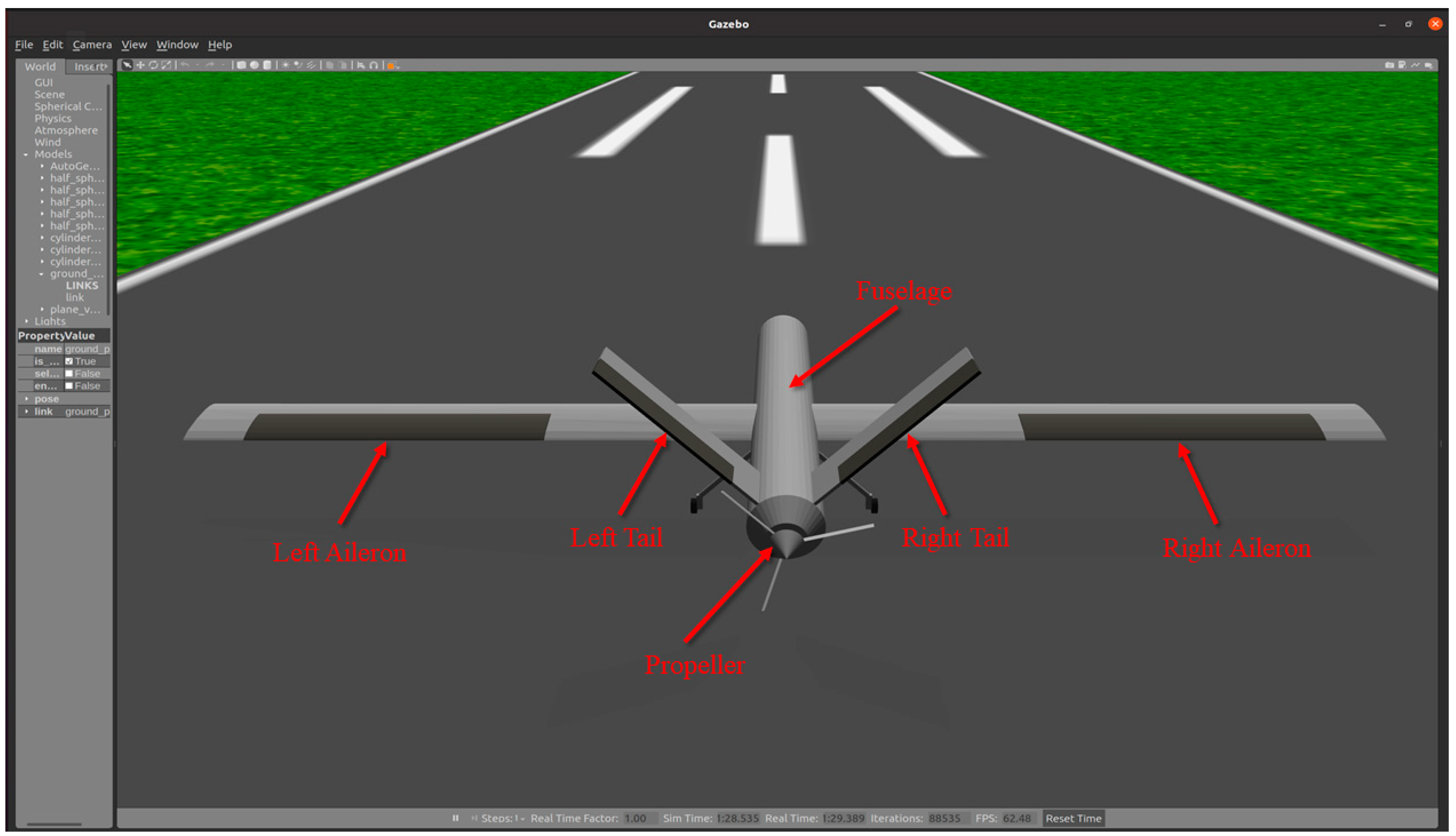
3.2. V-Tail Fixed-Wing UAV 3D Modeling

SolidWorks is a computer-aided design (CAD) software widely used for creating 3D models, assemblies, and drawings of various mechanical and engineering components, including aircraft. In the Gazebo simulation platform, there is no open-source V-tail aircraft available, and the official offering only includes the Cessna C-172 aircraft model. Therefore, we designed a V-tail aircraft using SolidWorks and configured the aerodynamics of our model through referencing the Cessna C-172 aircraft model files.
The aircraft model we built using SolidWorks is shown in Figure 1. This V-tail aircraft is modeled according to our reference to existing mainstream reconnaissance fixed-wing UAVs, such as the CAIG Wing Loong II and CASC Rainbow CH-4.
We rely on the aerodynamic plugin provided by the Gazebo simulator for the flight simulation of our aircraft model, which does not require the aircraft model to have an accurate aerodynamic shape, so we do not consider aerodynamic appearance when modeling in SolidWorks. At the same time, we omit the moving part modeling of the aircraft flaps, and we incorporate the functions of the flaps into the ailerons of the aircraft model.
In the Gazebo simulator, model description files are used to describe the objects in the simulation, including robots, UAVs, buildings, etc. The model description file contains the geometry of the object, physical properties, sensor information, and controllers, among others. Gazebo uses SDF (Simulation Description Format) as the default model description file format. SDF is an XML format used to describe simulation scenarios, which has rich functions and flexibility. In addition, URDF (Unified Robot Description Format) is a model description file format used in ROS. Gazebo can import URDF files with ROS plugin support and use the model in simulations.
In this project, we use the SDF file format as the aircraft model description file, because using SDF allows us to use the latest plugin provided by Gazebo. Stephen Brawner et al. developed a SolidWorks plugin for converting assembly models made in SolidWorks to URDF format [31]. Next, using the command line method provided by Gazebo [32], we can easily convert the model description file in URDF format to SDF format. Figure 2 shows the flow chart of converting a SolidWorks model to SDF format.
In the generated aircraft model file, we introduced an open-source aerodynamics plugin provided by Gazebo’s official sources [33]. This plugin’s mathematical model aligns with the aerodynamics mathematical model proposed in Section 3.1. Figure 3 shows the aerodynamic plugin used in the SDF model description file. The plugin has the following parameters to configure:
“a0” is the negative value of the zero-lift angle of attack.
“cla” is the slope of lift line.
“cda” is the slope of drag line.
“cma” is the slope of aerodynamic moment line.
“alpha_stall” is the stall angle of attack.
“cla_stall” is the slope of the lift line after stall.
“cda_stall” is the slope of the drag line after stall.
“cma_stall” is the slope of the aerodynamic torque line after stall.
“link_name” is the link applied by the aerodynamic force.
“cp” is the coordinate of the pressure center (in link coordinate system).
“aera” is the reference area of the aerodynamic surface.
“air_density” is the air density.
“forward” is the forward-direction vector (in link coordinate system).
“upward” is the up-direction vector (in link coordinates system).
“control_joint_name” is the name of the joint that controls the rudder axis.
“control_joint_rad_to_cl” is the rate of change of the lift coefficient with the control value.
If you intend to control models within Gazebo through an external program, there are typically two methods. The first involves creating a Gazebo plugin and embedding it into the model file you wish to control. However, this method lacks flexibility, and modifying plugin code can be cumbersome. The second method is for the external program to utilize Gazebo’s provided external interface, combined with ROS for controlling models in Gazebo and managing real-time simulation data for the models. In this study, we are using the second method. To incorporate ROS into the Gazebo simulation, we need to create a ROS launch file following ROS standards. This ROS launch file includes our V-tail aircraft model file, environment model file, and certain initialization parameters for Gazebo. Running this ROS launch file opens our aircraft simulation. Figure 4 depicts the initialization interface of the successfully opened simulation, where the aircraft model can be observed positioned on the runway.
We have chosen Gazebo as our aircraft simulator not only due to its capacity for customizing various simulation scenarios, but also for its support of simulating multiple models within a single scene. This feature provides a foundation for researching cooperative control algorithms for multi-agent systems. Figure 5 showcases our addition of nine V-tail aircraft within a single simulation scene.

4. 3D Flight Environment Design

Another focus of this study is the simulation modeling method tailored for obstacle avoidance in no-fly zones, providing a 3D flight scenario for aircraft models. The centerpiece of this scene is a large terrain model containing multiple mountain ranges. Custom no-fly zones are added, and wind disturbances are introduced to challenge the aircraft’s safe flight. These environmental models pose a challenge to ensuring the aircraft’s safe navigation.

4.1. Wind Disturbance

Wind disturbances can have significant effects on the behavior of an aircraft during flight, and it is crucial for pilots and control systems to account for these disturbances to ensure safe and stable operations. In this project, we mainly consider wind disturbances as gusts, steady wind, wind shear, and their combination.
Gusts refer to sudden and brief increases in wind speed that occur over a short period of time. These rapid changes in wind velocity can have significant effects on the flight performance and handling characteristics of aircraft. The mathematical representation of a discrete gust is:
V gusts   = { 0                                                                           x < 0 V m 2 ( 1 cos ( π x d m ) )         0 x d m V m                                                                   x > d m
where V m is the gust amplitude, d m is the gust length, x is the distance traveled, and V gusts   is the resultant wind velocity in the body axis frame.
Steady wind refers to a constant and uniform wind flow with consistent speed and direction over time. In the context of atmospheric conditions, it means that the wind is blowing at a steady rate and maintaining a constant heading for a significant period.
Wind shear refers to the change in wind speed and/or direction with altitude. It is a meteorological phenomenon that occurs in the Earth’s atmosphere and can affect aircraft during takeoff and landing. Strong wind shear can create turbulence and sudden changes in airspeed, making it challenging for pilots to maintain control and stability. The magnitude of the wind shear is given by the following equation for the mean wind profile as a function of altitude and the measured wind speed at 20 feet (6 m) above the ground.
V shear   = W 20 ln ( h z 0 ) ln ( 20 z 0 ) , 3 f t < h < 1000 f t
where V shear   is the mean wind speed, W 20 is the measured wind speed at an altitude of 20 feet, h is the altitude, and z 0 is a constant equal to 0.15 feet for Category C flight phases and 2.0 feet for all other flight phases. Category C flight phases are defined in reference [34] to be terminal flight phases, which include takeoff, approach, and landing.
In Gazebo, SDF plugins are used to extend the functionality of the simulation environment and add custom behavior to models or the world. SDF plugins are written in C++ and are loaded by Gazebo during the simulation startup.
In the simulation, the effect of wind disturbance on the aircraft can be regarded as a continuous external force acting on the body coordinates, and the wind disturbance model is packaged into an SDF plugin to activate it during simulation. To create a wind disturbance SDF plugin and add it to the aircraft flight environment, we typically follow these steps:
Step 1: Write the Plugin Code.
Create a C++ source file for the plugin and define the desired forces generated by wind disturbances acting on the body coordinate system.
Step 2: Build the Plugin.
Compile the plugin into a shared library (.so file) using CMake. Ensure that the plugin is linked to Gazebo and its required libraries.
Step 3: Load the Plugin.
In the Gazebo SDF file, include a “<plugin>” element that references the compiled plugin library and specifies any necessary parameters.
Figure 6 shows a wind plugin provided by Gazebo, which needs to have the following parameters to configure:
“linkName” is the link affected by the wind.
“xyzOffset” is the spatial offset of the link coordinate system to form the new coordinate system, which is the reference coordinate system for the wind.
“windDirection” is the force direction under the wind coordinate system.
“windForceMean” is the average value of the wind.
“windGustDirection” is the direction of the gust.
“windGustDuration” is the duration of the gust.
“windGustStart” is the start time of the gust.
“windGustForceMean” is the average value of the gust.

4.2. Terrain Model

Mountainous regions pose a threat to the safe flight of aircraft. When large fixed-wing UAVs are engaged in low-altitude penetration missions, their flight altitude is often relatively low. Aircraft must promptly adjust their flight altitude and course based on terrain obstacles to avoid collisions. In this section, we generate a large-scale terrain model using a heightmap.
In Gazebo, a heightmap is a type of terrain representation used to model the elevation and topography of the ground surface in a simulation environment. Heightmaps are an efficient way to create realistic and detailed terrains, especially for large outdoor scenes. A heightmap is essentially a 2D grid of elevation values, where each cell in the grid represents a point on the terrain, and the value in the cell determines the height or elevation of that point above a reference level, typically the ground level (Z = 0). The elevation values can be measured in meters, feet, or other units, depending on the scale of the simulation.
Figure 7 is a heightmap that we utilize. Essentially, it is a grayscale image. In the Gazebo environment model file, this heightmap can be configured to automatically generate the terrain model. In order for Gazebo to successfully load the heightmap and generate the terrain model, the original map needs to be cropped to the pixel size of (2n+1, 2n+1). In this project, the original heightmap was cropped to the pixel size of (1025, 1025).
At the same time, in order to make the generated terrain model more realistic, maps are used on the surface of the terrain. In the terrain model shown in Figure 8, three maps of water, grass, and sand are used, and different maps are used in different height threshold ranges. Figure 9 is a partial enlargement of the terrain model in Gazebo. The mountains in the figure are automatically generated terrain, and the height of the mountains can be scaled in the model profile.

4.3. No-Fly Zones

There are some areas where the flying of aircraft, drones, or other aerial vehicles is restricted or prohibited due to safety, security, or regulatory concerns. These zones are often established to prevent potential conflicts with other air traffic, protect sensitive areas, maintain privacy, and ensure public safety.
The restricted airspace designed in this study consists of multiple hemisphere models and cylindrical models. In our simulation scenario, the size and coverage of these no-fly zones are not fixed and remain dynamically deployable. The no-fly zone models are dynamically generated based on the terrain model designed in Section 4.2. Prior to launching the simulation program, we have the flexibility to customize the number, type, coverage area, and world coordinates of the no-fly zones. Therefore, a wide variety of different no-fly zone configurations can be applied on the same terrain model. Furthermore, during the aircraft flight simulation, it is possible to dynamically add additional no-fly zones to the original simulation environment. These zones can also be specified to undergo certain changes, such as translation with a fixed speed, based on predefined rules.
For the aircraft, the information about these no-fly zones is known. It can either be known to the aircraft before takeoff, including all the no-fly zones and threat areas, or it can be received in real-time by external perception devices (such as satellite remote sensing) through a data link. Based on this known information about no-fly zones and threat areas, the aircraft can plan its flight path in advance. When encountering newly acquired information about no-fly zones, the aircraft needs to perform dynamic avoidance maneuvers and replan its flight path accordingly.
The hemispherical no-fly zone model is formulated as follows:
L i ( x , y , z ) = ( x x i ) 2 + ( y y i ) 2 + z 2 = R R i m a x 2                         z 0
where the coordinate of the hemispherical no-fly zone i is ( x i ,   y i ,   z i ) , and R R i m a x is the maximum detection radius of the ground no-fly detector.
The Gazebo terrain model includes multiple hemispheres as no-fly zones, which can be customized in position, radius size, and color, as shown by the five red semi-transparent hemispheres in Figure 10.
The cylindrical no-fly zone model is formulated as follows:
L i ( x , y , z ) = ( x x i ) 2 + ( y y i ) 2 R M i m a x 2 = 0                         z i = [ 0 , Z i h ]
where L i ( x , y , z ) represents the hemispherical no-fly zone i , ( x i ,   y i ) represents the center coordinate of the cylinder i , R M i m a x represents the horizontal threat radius of the cylinder i , and Z i h represents the vertical threat altitude of the cylinder i .
Multiple cylinders are added to the Gazebo terrain model as no-fly zones; these cylinders are customizable in position, radius size, and color, as shown by the five purple translucent cylinders in Figure 11.

5. Comprehensive Simulation

In this section, we combine the V-tail aircraft designed in Section 3 with the flight threat scenario proposed in Section 4. The aircraft model performs flight simulation in the Gazebo simulator and collects and uses ROS to manage the data of the aircraft, such as position, attitude angle, angular velocity, and angular acceleration.
Figure 12 illustrates the main modules and primary data flow within the comprehensive simulation. Gazebo serves as the simulation platform for comprehensive control experiments of the V-tail aircraft, deployed within a large-scale 3D flight environment. We have designed two Python programs and use ROS for data management. The first program is utilized to retrieve the aircraft model’s state data in Gazebo at each simulation time step. It extracts the aircraft’s attitude and velocity data from the raw state data. The second program is responsible for controlling the desired state of the aircraft model. It includes attitude angle controllers and a flight speed controller, both employing PID control algorithms. These controllers output the deflection angles of the ailerons and V-tail, as well as the engine thrust magnitude, which are used to control the aircraft model in Gazebo.
The controller program for the V-tail fixed-wing UAV primarily consists of an attitude angle controller, flight speed controller, and altitude controller, as depicted in Figure 13. The attitude angle controller comprises three distinct control programs: pitch, roll, and yaw. The roll controller controls the aircraft’s roll angle through adjusting the aileron control surface. Both the pitch and yaw controllers use the deflection angles of the V-tail’s two control surfaces as outputs. Consequently, there is coupling between pitch and yaw control in V-tail aircraft. We use the pitch controller’s output control surface angle as a baseline, and the control surface angle output from the yaw controller is added to this baseline. This approach allows us to achieve yaw control while maintaining the desired pitch angle.
The flight speed controller adjusts the engine thrust to maintain the desired flight speed. The altitude hold controller is a two-loop controller, where the outer loop takes the desired altitude as input and outputs the pitch angle magnitude. The inner loop is the pitch angle controller. In this study, these controllers all use PID control algorithms.
In order to control the aircraft model in Gazebo from an external program, we established a link between ROS and Gazebo, as shown in Figure 14, where the oval box represents the ROS node and the connecting line represents the ROS topic, “/gazebo_gui” is the visual simulation interface of Gazebo, and “/gazebo” contains a variety of Gazebo simulation data, which is used to obtain and set the state of the model. “/object_position_publisher” retrieves multiple state data of the model from “/gazebo/model_states”, extracts the position and pose of the model, and publishes them through the topic “/plane_pose”. “/aircraft_command” publishes the angle and throttle controls of the aircraft, using three PID controllers to control the angles, corresponding to the pitch, roll, and yaw control of the aircraft. The desired angles are input by the keyboard key, and the controllers output the control values of the aircraft rudder surfaces.
Figure 15 depicts the comprehensive simulated flight environment, primarily composed of two terrain models. One is the runway model, utilized for taxiing and takeoff, while the other is the mountainous terrain model, simulating potential mountain obstacles that the aircraft may encounter during flight missions. We have designed an aircraft flight state controller program that enables control over the aircraft’s flight attitude angles and throttle through keyboard commands, as shown in Figure 16. The program continuously prints expected and actual flight states in real time. Using this control program, we have accomplished fundamental aircraft maneuvers such as climbing and rolling.
Figure 17 illustrates the simulated aircraft’s attitude angle data over a period of time. The deep blue line represents the roll angle data, the red line represents the pitch angle data, and the light blue line represents the yaw angle data. During the flight simulation, in conjunction with the flight controller program, the desired aircraft attitude angles are set through keyboard inputs. The attitude angle controller employs a PID control algorithm to manipulate the ailerons and V-tail to achieve the desired angles.
We tested the pitch angle controller of the aircraft. In the takeoff phase, the pitch angle was set to −0.3 radians, and the throttle was increased at the same time. The aircraft experienced overshoot and fluctuation in the pitch angle during the climbing phase, and finally stabilized at −0.3 radians as shown in Figure 18. Figure 19 shows the simulation screenshot of the aircraft in the climbing phase, and the PID controller of pitch angle outputs the maximum angular control (0.52 radians) to the tail. Figure 20 is a simulation screenshot of the aircraft reaching the pitch angle set point of −0.3 radians. In the pitch angle PID controller, set Kp = −3, Ki = −0.05, Kd = 0.05.
A PD controller is employed for the aircraft’s roll angle control, with PD controller parameters set as follows: Kp = −5 and Kd = −0.05. Figure 21 displays the roll angle curve of the aircraft, demonstrating that the use of the PD controller effectively stabilizes the aircraft’s roll angle. It’s important to note that the roll angle control involves a system with significant delays. This is why we opted not to introduce integral control, as it could potentially affect the stability of the control system. Figure 22 depicts a 3D simulation snapshot of the aircraft’s roll angle stabilizing at 0.42 radians.

6. Conclusions

Nowadays, large fixed-wing UAVs are being utilized for a variety of tasks. Relevant research indicates that V-tail configurations can effectively reduce aerodynamic drag and enhance flight endurance. However, achieving efficient customized development and various intelligent functionalities in a specific domain remains an unresolved challenge. This study integrates SolidWorks model design with aircraft simulation technology, establishing a comprehensive aircraft simulation system in Gazebo that encompasses kinematics, dynamics, and collision characteristics. Additionally, a simulation environment modeling approach for obstacle avoidance in no-fly zones is presented, creating a large-scale flight environment model that includes mountains, wind disturbances, and no-fly zones. Data communication and motion control are achieved through ROS, and the aircraft’s attitude control is implemented using a PID algorithm. The primary contribution of this research lies in providing a 3D visualization simulation platform for dynamic obstacle avoidance, trajectory planning, and formation flying applications in the context of large-scale fixed-wing unmanned aircraft.
Currently, this research is at the initial stage, and there is still a lot of work to be done. The following outlines the future directions of the study:
(1)
Develop trajectory planning and tracking algorithms for the research aircraft to achieve obstacle avoidance flight with minimal cost.
(2)
Investigate multi-aircraft formation flying algorithms, aiming to maintain formation while avoiding threat areas as effectively as possible.

Author Contributions

Conceptualization, P.H. and T.W.; methodology, Y.T. and P.H.; software, P.H.; validation, B.Y. and P.H.; formal analysis, P.H.; investigation, P.H. and T.W.; resources, T.W. and Y.T.; writing—original draft preparation, P.H.; writing—review and editing, P.H. and T.W.; visualization, P.H. and B.Y.; supervision, T.W.; project administration, T.W.; funding acquisition, T.W. All authors have read and agreed to the published version of the manuscript.

Funding

This research received no external funding.

Data Availability Statement

The data are not publicly available.

Conflicts of Interest

The authors declare no conflict of interest.

References

  1. Khan, M.U.; Khan, M.D.; Din, N.A.; Babar, M.Z.; Hussain, M.F. Aerodynamic Comparison of Unconventional Aircraft Tail Setup. In Proceedings of the 2019 22nd International Multitopic Conference (INMIC), Islamabad, Pakistan, 29–30 November 2019; pp. 1–5. [Google Scholar] [CrossRef]
  2. Vatandas, O.E.; Anteplioglu, A. Aerodynamic performance comparison of V-tail and conventional tail for an unmanned vehicle. In Proceedings of the 2015 7th International Conference on Recent Advances in Space Technologies (RAST), Istanbul, Turkey, 16–19 June 2015; pp. 655–658. [Google Scholar] [CrossRef]
  3. Zountouridou, E.; Kiokes, G.; Dimeas, A.; Prousalidis, J.; Hatziargyriou, N. A guide to unmanned aerial vehicles performance analysis—The MQ-9 unmanned air vehicle case study. J. Eng. 2023, 2023, e12270. [Google Scholar] [CrossRef]
  4. Kim, S.; Park, J.; Yun, J.-K.; Seo, J. Motion Planning by Reinforcement Learning for an Unmanned Aerial Vehicle in Virtual Open Space with Static Obstacles. In Proceedings of the 2020 20th International Conference on Control, Automation and Systems (ICCAS), Busan, Republic of Korea, 13–16 October 2020; pp. 784–787. [Google Scholar] [CrossRef]
  5. Rivera, Z.B.; De Simone, M.C.; Guida, D. Unmanned Ground Vehicle Modelling in Gazebo/ROS-Based Environments. Machines 2019, 7, 42. [Google Scholar] [CrossRef]
  6. Sokolov, M.; Lavrenov, R.; Gabdullin, A.; Afanasyev, I.; Magid, E. 3D modelling and simulation of a crawler robot in ROS/Gazebo. In Proceedings of the 4th International Conference on Control, Mechatronics and Automation, Barcelona, Spain, 7–11 December 2016; pp. 61–65. [Google Scholar]
  7. Bingham, B.; Agüero, C.; McCarrin, M.; Klamo, J.; Malia, J.; Allen, K.; Lum, T.; Rawson, M.; Waqar, R. Toward Maritime Robotic Simulation in Gazebo. In Proceedings of the OCEANS 2019 MTS/IEEE SEATTLE, Seattle, WA, USA, 27–31 October 2019; pp. 1–10. [Google Scholar] [CrossRef]
  8. Niu, C.; Yan, X.; Chen, B. Control-oriented modeling of a high-aspect-ratio flying wing with coupled flight dynamics. Chin. J. Aeronaut. 2023, 36, 409–422. [Google Scholar] [CrossRef]
  9. Jayaraman, B.; Saini, V.K.; Ghosh, A.K. Robust Time-Delayed PID Flight Control for Automatic Landing Guidance under Actuator Loss-Of-Control. IFAC-PapersOnLine 2022, 55, 189–194. [Google Scholar] [CrossRef]
  10. Xu, B.; Zhang, Q.; Pan, Y. Neural network based dynamic surface control of hypersonic flight dynamics using small-gain theorem. Neurocomputing 2016, 173, 690–699. [Google Scholar] [CrossRef]
  11. Morton, S.A.; McDaniel, D.R. A Fixed-Wing Aircraft Simulation Tool for Improving DoD Acquisition Efficiency. Comput. Sci. Eng. 2016, 18, 25–31. [Google Scholar] [CrossRef]
  12. Deiler, C.; Kilian, T. Dynamic aircraft simulation model covering local icing effects. CEAS Aeronaut. J. 2018, 9, 429–444. [Google Scholar] [CrossRef]
  13. Heesbeen, B.; Ruigrok, R.; Hoekstra, J. GRACE-a Versatile Simulator Architecture Making Simulation of Multiple Complex Aircraft Simple. In Proceedings of the AIAA Modeling and Simulation Technologies Conference and Exhibit, Keystone, CO, USA, 21–24 August 2006; p. 6477. [Google Scholar]
  14. Aschauer, G.; Schirrer, A.; Kozek, M. Co-simulation of matlab and flightgear for identification and control of aircraft. IFAC-PapersOnLine 2015, 48, 67–72. [Google Scholar] [CrossRef]
  15. Yang, L.; Hu, B.; Fu, J.; Fu, Y. Research on Longitudinal Control and Visual Simulation System for Civil Aircraft Based on Simulink/FlightGear. In Proceedings of the 2022 Chinese Intelligent Systems Conference. CISC 2022, Beijing, China, 15–16 October 2022; Lecture Notes in Electrical Engineering. Jia, Y., Zhang, W., Fu, Y., Zhao, S., Eds.; Springer: Singapore, 2022; Volume 951. [Google Scholar] [CrossRef]
  16. Rostami, M.; Kamoonpuri, J.; Pradhan, P.; Chung, J. Development and Evaluation of an Enhanced Virtual Reality Flight Simulation Tool for Airships. Aerospace 2023, 10, 457. [Google Scholar] [CrossRef]
  17. Marianandam, P.A.; Ghose, D. Vision based alignment to runway during approach for landing of fixed wing uavs. IFAC Proc. Vol. 2014, 47, 470–476. [Google Scholar] [CrossRef]
  18. Henry, D. Application of the H∞ control theory to space missions in engineering education. IFAC-PapersOnLine 2020, 53, 17132–17137. [Google Scholar] [CrossRef]
  19. Horri, N.; Pietraszko, M. A Tutorial and Review on Flight Control Co-Simulation Using Matlab/Simulink and Flight Simulators. Automation 2022, 3, 486–510. [Google Scholar] [CrossRef]
  20. Bittar, A.; Figuereido, H.V.; Guimaraes, P.A.; Mendes, A.C. Guidance Software-In-the-Loop simulation using X-Plane and Simulink for UAVs. In Proceedings of the 2014 International Conference on Unmanned Aircraft Systems (ICUAS), Orlando, FL, USA, 27–30 May 2014; pp. 993–1002. [Google Scholar] [CrossRef]
  21. Çetin, E.; Kutay, A.T. Automatic landing flare control design by model-following control and flight test on X-Plane flight simulator. In Proceedings of the 2016 7th International Conference on Mechanical and Aerospace Engineering (ICMAE), London, UK, 18–20 July 2016; pp. 416–420. [Google Scholar] [CrossRef]
  22. Aláez, D.; Olaz, X.; Prieto, M.; Porcellinis, P.; Villadangos, J. HIL Flight Simulator for VTOL-UAV Pilot Training Using X-Plane. Information 2022, 13, 585. [Google Scholar] [CrossRef]
  23. Yang, J.; Thomas, A.G.; Singh, S.; Baldi, S.; Wang, X. A Semi-Physical Platform for Guidance and Formations of Fixed-Wing Unmanned Aerial Vehicles. Sensors 2020, 20, 1136. [Google Scholar] [CrossRef] [PubMed]
  24. Irmawan, E.; Harjoko, A.; Dharmawan, A. Model, Control, and Realistic Visual 3D Simulation of VTOL Fixed-Wing Transition Flight Considering Ground Effect. Drones 2023, 7, 330. [Google Scholar] [CrossRef]
  25. Lee, J.; Spencer, J.; Paredes, J.A.; Ravela, S.; Bernstein, D.S.; Goel, A. An adaptive digital autopilot for fixed-wing aircraft with actuator faults. arXiv 2021, arXiv:2110.11390. [Google Scholar]
  26. Lee, J.; Spencer, J.; Shao, S.; Paredes, J.A.; Bernstein, D.S.; Goel, A. Experimental Flight Testing of a Fault-Tolerant Adaptive Autopilot for Fixed-Wing Aircraft. In Proceedings of the 2023 American Control Conference (ACC), San Diego, CA, USA, 31 May–2 June 2023; pp. 2981–2986. [Google Scholar] [CrossRef]
  27. Ellingson, G.; McLain, T. ROSplane: Fixed-wing autopilot for education and research. In Proceedings of the 2017 International Conference on Unmanned Aircraft Systems (ICUAS), Miami, FL, USA, 13–16 June 2017; pp. 1503–1507. [Google Scholar] [CrossRef]
  28. Stevens, B.L.; Lewis, F.L.; Johnson, E.N. Aircraft Control and Simulation: Dynamics, Controls Design, and Autonomous Systems; John Wiley & Sons: Hoboken, NJ, USA, 2015. [Google Scholar]
  29. Babister, A.W. Aircraft Dynamic Stability and Response: Pergamon International Library of Science, Technology, Engineering and Social Studies; Elsevier: Amsterdam, The Netherlands, 2013. [Google Scholar]
  30. Sinha, N.K.; Ananthkrishnan, N. Elementary Flight Dynamics with an Introduction to Bifurcation and Continuation Methods; CRC Press: Boca Raton, FL, USA, 2021. [Google Scholar]
  31. SolidWorks to URDF Exporter. Available online: https://wiki.ros.org/sw_urdf_exporter (accessed on 15 July 2023).
  32. Convert URDF to SDF. Available online: https://answers.gazebosim.org//question/2282/convert-urdf-to-sdf-or-load-urdf/ (accessed on 15 July 2023).
  33. Gazebo’s Aerodynamics Tutorial. Available online: https://classic.gazebosim.org/tutorials?tut=aerodynamics&cat=physics (accessed on 25 August 2023).
  34. Moorhouse, D.J.; Woodcock, R.J. Background Information and User Guide for MIL-F-8785C, Military Specification: Flying Qualities of Piloted Airplanes. 1982. Available online: https://apps.dtic.mil/sti/citations/tr/ADA119421 (accessed on 10 September 2023).
Figure 1. A 3D model of a V-tail fixed-wing UAV created using SolidWorks. The aircraft model has 8 moving parts, which are ① right aileron, ② left aileron, ③ right tail, ④ left tail, ⑤ propeller, ⑥ front wheel, ⑦ right wheel, and ⑧ left wheel.
Drones 07 00601 g001
Figure 2. Flowchart of converting a SolidWorks model to SDF format. In SolidWorks, individual 3D models of different components of the aircraft are created separately. These components are then assembled to form a complete aircraft. A model format conversion plugin is used to convert this model into URDF format. Finally, the model is converted to the SDF format recommended by Gazebo using the format conversion command in the terminal.
Drones 07 00601 g002
Figure 3. Add aerodynamic plugin to the SDF aircraft model description file. Using the official aerodynamics plugin provided by Gazebo, the figure displays the aerodynamic parameters of the left wing. In the aircraft model description file used in this study, the same plugin is also employed for the right wing and tails.
Drones 07 00601 g003
Figure 4. V-tail aircraft in Gazebo. After successfully launching the simulation program, the aircraft model will appear on the runway scene in Gazebo.
Drones 07 00601 g004
Figure 5. Multiple V-tail aircraft in Gazebo. Gazebo supports the simultaneous simulation of multiple aircraft models, which facilitates the research of multi-UAV formation flight algorithms.
Drones 07 00601 g005
Figure 6. Add wind plugin to the SDF aircraft model description file. Using the officially provided wind disturbance plugin, you can set the wind direction and magnitude for both constant wind and gusts.
Drones 07 00601 g006
Figure 7. Original heightmap. Different grayscale values represent different altitudes, where higher grayscale values (whiter pixels) indicate higher elevations.
Drones 07 00601 g007
Figure 8. Terrain model in Gazebo. Different textures are applied to different altitudes: blue texture represents ocean areas, green texture represents grassland regions, and brown texture represents mountainous areas.
Drones 07 00601 g008
Figure 9. Terrain model in Gazebo (local zoom). The image displays details from Figure 8, where the red dashed box highlights mountains at different altitudes. These mountains pose a threat to low-altitude aircraft flight.
Drones 07 00601 g009
Figure 10. Hemisphere models in Gazebo. On the foundation of the terrain model, some custom semi-transparent red hemisphere regions are added as no-fly zones.
Drones 07 00601 g010
Figure 11. Cylinder models in Gazebo. On the foundation of the terrain model, some custom semi-transparent purple cylindrical regions are added as no-fly zones.
Drones 07 00601 g011
Figure 12. The comprehensive simulation system flowchart.
Drones 07 00601 g012
Figure 13. The block diagram for the V-tail aircraft controller design.
Drones 07 00601 g013
Figure 14. ROS node graph. Using the official ROS tool, “rqt_graph” generates a ROS node graph, where ellipses represent individual nodes and arrows indicate the direction of data transmission.
Drones 07 00601 g014
Figure 15. Comprehensive simulation flight scenario. The flight environment consists of two parts: one is the runway scene used for taxiing and takeoff of the aircraft, and the other is the terrain model used to simulate obstacles encountered by the aircraft during flight.
Drones 07 00601 g015
Figure 16. Keyboard control. The figure displays an aircraft control program we designed, which allows controlling the aircraft’s attitude and throttle through keyboard inputs. It also prints the desired and actual values in real time.
Drones 07 00601 g016
Figure 17. Attitude angle data of the aircraft. During flight testing, a segment of attitude angle data is recorded. Through configuring different desired attitude angles, the attitude angle controller steers the aircraft to reach the desired angles.
Drones 07 00601 g017
Figure 18. Pitch angle data of the aircraft. Pitch angle data during the aircraft’s takeoff phase is recorded. At the moment of takeoff, the desired pitch angle is set to −0.3 radians. After a period of angular fluctuations, the pitch angle eventually stabilizes at −0.3 radians.
Drones 07 00601 g018
Figure 19. Aircraft is in the climbing phase. The aircraft’s V-tail control surface is set to rotate within the range of −0.52 radians to 0.52 radians. At takeoff, the pitch angle is set to −0.3 radians, at which point the V-tail control surface is at its maximum deflection.
Drones 07 00601 g019
Figure 20. The pitch angle of the aircraft is stable at −0.3 radians. When the aircraft’s pitch angle stabilizes at −0.3 radians, due to excessive lift, the V-tail control surface needs to rotate downward by a certain angle to maintain pitch stability.
Drones 07 00601 g020
Figure 21. Roll angle data of the aircraft. During the stable flight phase, multiple desired roll angles for the aircraft are set to evaluate the performance of the roll angle controller.
Drones 07 00601 g021
Figure 22. The roll angle of the aircraft is stable at 0.42 radians. A screenshot of the aircraft maintaining a roll angle of 0.42 radians is taken. At this moment, the aileron control surface is essentially not deflected. Due to excessive lift generated by the high aircraft speed, the V-tail control surface rotates downward by a certain angle to maintain pitch stability.
Drones 07 00601 g022
Disclaimer/Publisher’s Note: The statements, opinions and data contained in all publications are solely those of the individual author(s) and contributor(s) and not of MDPI and/or the editor(s). MDPI and/or the editor(s) disclaim responsibility for any injury to people or property resulting from any ideas, methods, instructions or products referred to in the content.

