Drone-Based Vertical Atmospheric Temperature Profiling in Urban Environments

Abstract

The accurate and detailed measurement of the vertical temperature, humidity, pressure, and wind profiles of the atmosphere is pivotal for high-resolution numerical weather prediction, the determination of atmospheric stability, as well as investigation of small-scale phenomena such as urban heat islands. Traditional approaches, such as weather balloons, have been indispensable but are constrained by cost, environmental impact, and data sparsity. In this article, we investigate uncrewed aerial systems (UASs) as an innovative platform for in situ atmospheric probing. By comparing data from a drone-mounted semiconductor temperature sensor (TMP117) with traditional radiosonde measurements, we spotlight the UAS-collected atmospheric data’s accuracy and such system suitability for atmospheric surface layer measurement. Our research encountered challenges linked with the inherent delays in achieving ambient temperature readings. However, by applying specific data processing techniques, including smoothing methodologies like the Savitzky–Golay filter, iterative smoothing, time shift, and Newton’s law of cooling, we have improved the data accuracy and consistency. In this article, 28 flights were examined and certain patterns between different methodologies and sensors were observed. Temperature differentials were assessed over a range of 100 m. The article highlights a notable accuracy achievement of 0.16 ± 0.014 °C with 95% confidence when applying Newton’s law of cooling in comparison to a radiosonde RS41’s data. Our findings demonstrate the potential of UASs in capturing accurate high-resolution vertical temperature profiles. This work posits that UASs, with further refinements, could revolutionize atmospheric data collection.

1. Introduction

The measurement of the vertical profiles of atmospheric temperature, humidity, pressure, and wind is important for determining atmospheric stability. Air pollutants might become trapped in stable atmospheric layers due to the absence of convective currents and an increase in concentration, thus introducing human health hazards [1]. An urban heat island (UHI) is a region of higher-than-ambient temperature in an urban environment caused by condensed build-up, altered terrain, and materials of high albedo such as asphalt, which has a significant effect on the wellbeing of the people living nearby [2]. An efficient way to explore the vertical structure of UHIs is using a UAS. This might provide valuable data for urban planning purposes, which might help mitigate this undesirable phenomenon [3]. According to Sun et al., soundings using a UAS also improve the numerical weather prediction results in unpopulated regions [4].

Weather balloons are the conventional means of atmospheric sampling; however, their uncontrollable and mostly disposable nature translates to high cost for the operator and the environment in the form of pollution by latex, batteries, and other electronic components [5], since only about 20% of the released sondes are recovered [6], while UASs are reusable by nature and are lost only in the rare case of an accident. Furthermore, according to Pinto et al. [7], measurements made by weather balloons are sparse both temporally (most meteorological stations launch radiosondes attached to weather balloons twice daily and some once) and spatially (it is not uncommon for launching sites to be spaced more than 300 km apart even in developed countries), which leaves a huge gap of information needed for more accurate models and forecasts of weather.

Each launch of a balloon-tethered radiosonde incurs an estimated cost of approximately 500 €, encompassing expenses associated with the acquisition of requisite equipment, lighter-than-air gases, maintenance personnel, and miscellaneous overheads. In contrast, drone technology represents a substantially more cost-effective alternative, affording nations the opportunity to curtail expenses related to meteorological data acquisition or enhance the data gathering density. For instance, employing a DJI M300 drone facilitates a flight at an approximate cost of 200 €, or even less. Our calculations, supported by reference [8], encompass all the essential components, encompassing the procurement of necessary equipment, DJI Care Plus drone insurance, constrained battery usage limited to 300 cycles, preemptive propeller and motor replacements, and carbon fiber arm refurbishments, as well as an annual drone replacement policy. The daily operational expenses for this drone, exclusive of operator-related costs, amount to approximately 60 €, thereby rendering operator expenses the most prominent cost factor. However, the reduction of this expenditure is feasible through further technological advancements, such as the implementation of fully autonomous missions coupled with automatic charging stations. Such technology for autonomous drone recharging and launch already exists, as cited in reference [9], albeit a comprehensive meteorological solution for the lower atmospheric boundary layer is still in the developmental stages. If fully integrated, this technology would necessitate periodic inspections, leading to a substantial reduction in operational costs. The cost of the materials used to develop the sensing system are in the order of 100 €, including the sensors, logging unit, and batteries. In theory, such system could be attached to other vehicles than the M300. The systems described in other authors’ work [10,11] cost around 1500 € and 500 €, respectively, including the vehicle.

Aircraft Meteorological Data Relay (AMDAR) is a component system of the World Meteorological Organization (WMO)’s Integrated Global Observing System, contributing commercial aircraft-based observations to the World Weather Watch Program [12]. Nonetheless, aircraft usually fly on predefined routes, especially during the initial climb and approach phases, which limits the spatial data availability to a narrow strip aligned with the runway, especially close to the ground. Several studies [4,7,11,13,14,15,16,17,18] advocate for the adoption of UASs for in situ atmospheric probing, highlighting their cost-effectiveness, mobility, and reusability.

Furthermore, the WMO has announced a campaign aiming to evaluate the use of UASs in operational meteorology in order to address the in situ observational gap surface layer, atmospheric boundary layer, and lower free troposphere. Data from processes that occur at much finer spatio-temporal scales than currently captured by conventional, operational observing systems need to be captured. According to one white paper [19], UASs are now capable of collecting routine observations of the lower atmosphere to extend existing observing system networks. The wider applicability of UASs in operational meteorology was made possible by recent advancements in battery technology, which enabled a transition from internal combustion to electrically powered vehicles, offering both lower upfront and maintenance costs. Advances in control technology have simplified flight automation, which offers a reliable and repeatable data acquisition process. UAVs have used increasingly miniaturized and accurate sensors with radiation shielding, insulation, and aspiration. This has led to results comparable in accuracy to other meteorological instruments, such as radiosondes in the upper part of the boundary layer. However, standards for accuracy, data quality, sampling rates, and data frequency have not yet been established. The reusable vehicle platform offers great cost efficiency as mentioned previously. Some of the other unsolved problems include the following: flyability, the ability to perform soundings even in harsh conditions; automation reliability; safety in case of an accident; airspace integration, which would expedite the process of obtaining permissions to fly at higher altitudes; and the lack of an internationally recognized standard data format. Demonstrations of UASs in an operational environment have been limited in scope and duration. The campaign is planned to launch in 2024 and demonstrate the current capabilities of weather UASs and data processing systems, as well as investigate the impacts of such systems on relevant application areas and determine the areas of systems and regulatory conditions that need further improvement for the integration of UASs into the meteorological network. In this paper, we delve deeper into the problem of UAV-based data accuracy and resolution in the lower boundary (surface) layer of the atmosphere using measurements with radiosonde data and exploring solutions to enhance the accuracy and reliability of these measurements. An evaluation of such a system near the surface has not been found in other authors’ work.

Weather balloons ascend at rates between 4 and 6 m/s at altitudes below 10 km [20]. In contrast, drones exhibit a wide range of vertical climb speeds, ranging from less than 1 m/s to over 30 m/s. The experiments in this study used a DJI Matrice 300RTK with maximum vertical speed of 6 m/s [21]. Climb speed control is relevant when considering thermal inertia, the ability for readings to change gradually when placed in a different environment as the sensor adjusts to the new temperature. Counteracting the small size of the sensor and the constant airflow around it is beneficial. To reduce thermal inertia further, authors use data processing methods such as time shift and averaging [22]. Another method proposed by [13] uses the temperature reading and the rate of change in the reading to predict the actual ambient temperature. After correction, the authors were able to achieve a root mean square error (RMSE) between ascent and descent equal to 0.2 °C. This is relevant because inertial errors between the values measured during the ascent and descent form a hysteresis loop.

A review of the literature describing temperature soundings taken using UASs was made. Here are relevant examples:

Lawrence et al. [11] have developed a small airborne measurement system (SAMS) for monitoring turbulence as well as temperature and humidity in the atmospheric boundary layer (ABL) and above. It features a 0.7 kg, 1 m wingspan flying wing configuration airframe with such sensors attached: a cold-wire temperature sensor (resolution: <0.003 °C, accuracy: 2 °C, time constant: 0.5 ms), a semiconductor temperature sensor (resolution: 0.1 °C, accuracy: 2 °C, time constant: 5 s), and a relative humidity sensor (resolution: 0.01%, accuracy: 2%, time constant: 5 s). The measurement system proposed costs around 500 €, including the vehicle and the sensing equipment. It does not seem to include the cost of the ground control station (computers and radio equipment) and launching equipment (bungee launch and meteorological balloon).

Hemingway et al. [23] used a Matrice 600, a hexacopter measuring 1.13 m in diameter and weighing 9.1 kg with a 7 kg payload capacity. It was fitted with a Young Model 81,000 ultrasonic anemometer, capable of measuring ambient temperature with errors of less than 1% in typical conditions. The horizontal temperature profiles were treated as time series and converted into spatial domains by applying Taylor’s hypothesis and the mean ground speed or the true air speed. Due to the different nature of measurement (speed of sound calculation), the ultrasonic sensor is not susceptible to inertia and therefore the time constant can be said to be equal to the sampling rate (32 Hz in case of the Young Model 81000).

Gapski et al. [24] found that surface reflectance plays an important role in the formation of UHIs. Roofs, facades, and pavement were the most significant contributors depending on the season (sun incidence angle) and the height and density of the buildings. Conclusions were drawn from the data collected by stationary HOBO MX1101 thermometer loggers (accuracy: 0.21 °C, resolution: 0.024 °C) placed 4.5 m above ground level, as well as computer simulations created using ENVI-met version 4.4.6 model. The measurements were taken during spring and winter. It was concluded that the solar reflectance of facades had a greater impact on the temperature variation in denser areas. Roofing and paving surfaces are more critical in open spaces.

Chiliński et al. [15] took measurements of black carbon concentrations in the low-level atmosphere in Warsaw, Poland, during the cold season. Fumes escaping the chimneys of heated households were measured during temperature inversions as this phenomenon prevents atmospheric layer mixing as well as solid particle escape. The sensor used for black carbon sensing was a microAeth^®/AE51 device weighing ~200 g and capable of autonomous operation, requiring no additional power supply or logging device. For thermodynamical measurements, a Vaisala RS92-SG radiosonde was used. It features a temperature sensor with a <0.4 s response time at 6 m/s airflow and 100–1000 hPa ambient pressure as well as 0.2 °C of accuracy during reproducibility in sounding at 100–1080 hPa of pressure with a resolution of 0.1 °C. The relative humidity sensor of the radiosonde offered a resolution of 1% with a response time of <0.5 s at 20 °C and an accuracy of 2%. The devices were mounted on a Versa X6sci hexacopter. The final weight of the system was 3.5 kg, of which 490 g were due to the measuring equipment. The flight time of the system was around 12 min. Researchers have found a correlation between the temperature inversion height and intensity and black carbon concentrations. Also, the concentration vertical profiles were examined using a UAS, which was useful information not accessible to a terrestrial lidar at low altitudes.

Lee et al. [16] have performed similar experiments related to black carbon concentrations and temperature inversion. During the campaign, the same microAeth^®/AE51 carbon sensing device was used. For temperature sensing, Testo 174 sensors (measuring rate: 1 min–24 h, temperature accuracy: ±0.5 °C, temperature resolution: 0.1 °C, humidity accuracy: ±3% at +25 °C, humidity resolution: 0.1%) were utilized. The sensors were attached to a hexacopter, assembled using a DJI F550 frame (550 mm diameter). The whole system weighed around 2 kg and could operate for 13–15 min. The maximum operation altitude was about 1000 m, while the maximum horizontal and vertical velocities were both 14 m/s. The measurements were performed in three different manners: at random, where measurement altitudes were chosen in a random order and the drone would fly a sequence of these altitudes; ascending, where the drone would ascend from the ground level up to 130 m above ground level (AGL); and descending, which would commence at 130 m AGL and descend to the ground level.

Lee et al. [25] used two UASs, the Meteodrone MM-641/SSE and Black Swift S2, the former of which is a 40 cm diameter hexacopter capable of a 12 min flight time, 3 m/s ascent, and up to a 20 m/s descent speed with a system weight of 0.7 kg, and the latter being a 3 m wingspan fixed-wing aircraft, with a maximum take-off weight of 9.5 kg and 2.3 kg payload capacity. During one of the flights, the vertical temperature profiles up to 350 m above ground measured using both platforms agreed to within 0.2 °C. The sensor characteristics of the Meteodrone were not provided. An iMet-XQ2 sensor module (temperature response time: 1 s at 5 m/s flow, accuracy: +/− 0.3 °C, resolution: 0.01 °C, humidity response time: 0.6 s at 25 °C, accuracy: +/− 5%, resolution: 0.1%) was attached to the Black Swift.

Prior et al. [17] used a Kestrel DROP D3FW Fire Weather Monitor (temperature accuracy: 0.5 °C, temperature resolution: 0.1 °C, humidity accuracy: 2%, humidity resolution: 0.1%, wet-bulb globe temperature response time: 160 s) attached via a 7.6 m long fishing line to the landing gear of Autel Robotics X-Star Premium and DJI Phantom 4 Pro V2.0 quadcopters, both similar in dimensions (~350 mm diagonal) and flight endurance (~25 min). During each flight, the altitude was limited to 122 m AGL to comply with the regulations. The sUASs rose vertically upward at 1 m/s to the maximum altitude desired for each flight. It was then flown at that same altitude to one of the sample sites. Once over the sample site, the sUAS was then lowered at approximately 1 m/s until the sensors were as close to the desired canopy as possible. The sUAS was then flown vertically upward at 1 m/s back to the maximum altitude. Other nearby sample sites were then visited, and vertical profiles were taken using the same procedure. The gathered data were processed such that any values recorded in a two-meter interval were averaged and assigned to a particular altitude to correspond to the 1 m/s vertical speed and the 2 s sampling interval. The measurements were repeated several times above different surfaces (parking lot, forest, pasture, lake). The study concluded that anomalies occurred consistently up to ~20 m AGL, which can be attributed to landcover. It was observed that the air temperature increased by up to several degrees close to paved surfaces and decreased over a lake. Other influences were attributed to steep topography. Besides these, the profiles tended to follow standard adiabatic lapse rates except for inversion events.

Hervo et al. [18] have published the results of a campaign in which atmospheric measurements from a Meteodrone MM-670 (flight time: ~22 min, diameter: 70 cm, weight: 5 kg), a hexacopter manufactured by Meteomatics, were compared to measurements taken by a weather balloon-tethered radiosonde (RS41 by Vaisala) as well as remote sensing equipment (microwave radiometer, Raman lidar). The UAS was launched every hour between 20:00 and 04:00 UTC during working days, while the sonde was launched every day at 11:00 and 23:00 UTC. It was found that the drone measurements deviated from the radiosonde by a RMSE of 0.68 °K for temperature and 8.3% for relative humidity. The World Meteorological Organization (WMO) requirements for the accuracy of measurements used for atmospheric climate forecasting and monitoring are categorized into three levels: “threshold” (1 °K, 1%) is the minimum requirement for the data to be useful, “goal” (0.1 °K, 0.1%) is the limit above which further improvements are not more beneficial for the given application, and “breakthrough” (0.5 °K, 0.5%) is an intermediate level between “threshold” and “goal” which, if achieved, would result in a significant improvement for the targeted application [26]. The error of the radiosonde was assumed to be negligible.

Sun et al. [4] conducted experiments involving the assimilation of radiosonde and meteorological drone data into NWP models. The drone used was a small unmanned meteorological observer (SUMO) based on a fixed-wing frame from Multiplex (80 cm wingspan, <30 min endurance) and incorporating autopilot and meteorological sensors from Lindenberg und Müller. For meteorological sensing, two sensor combinations, both measuring temperature and relative humidity, were used: the DigiPicco I2C from IST (relative humidity sensing resolution: 0.003%, accuracy: <3%, response time: 5 s; temperature resolution: 0.005 °K, accuracy: 0.5 °K, response time: unknown) and the SHT75 from Sensirion (relative humidity sensing resolution: 0.03%, accuracy: 1.8%, response time: 6 s; temperature resolution: 0.01 °K, accuracy: 0.5 °K, response time: 5 s) [10]. The results have shown that the assimilation of the data gathered by a radiosonde or SUMO has a clear positive effect on local weather analyses, and in many cases, the benefit extends farther than 300 km. The impact of the radiosonde soundings was found to be larger, which was attributed to the fact that the vertical measurement extent was much larger (~12 km) than the one achievable by the SUMO (~2 km). In addition, whereas radiosondes primarily ascend vertically at fixed rates, UASs boast the versatility to navigate both vertically and horizontally. This expanded range of motion provides researchers with the opportunity to conduct experiments on horizontal temperature gradients, which is particularly useful when analyzing urban heat islands.

To summarize, the temperature measurement methods include continuous ascent and descent [1,4,11,17,18,23], which enables averaging between the ascent and descent and decreases the inertial errors. This seems to be the dominant method in temperature profile collection. It is used in this work as well. Hemingway et al. [14] have used only data from the ascent, since averaging of the results might skew the special structure due to temporal variations, which were important in the study. Stepped constant altitude measurement can be used if temporal variations at one altitude are of importance [11]. 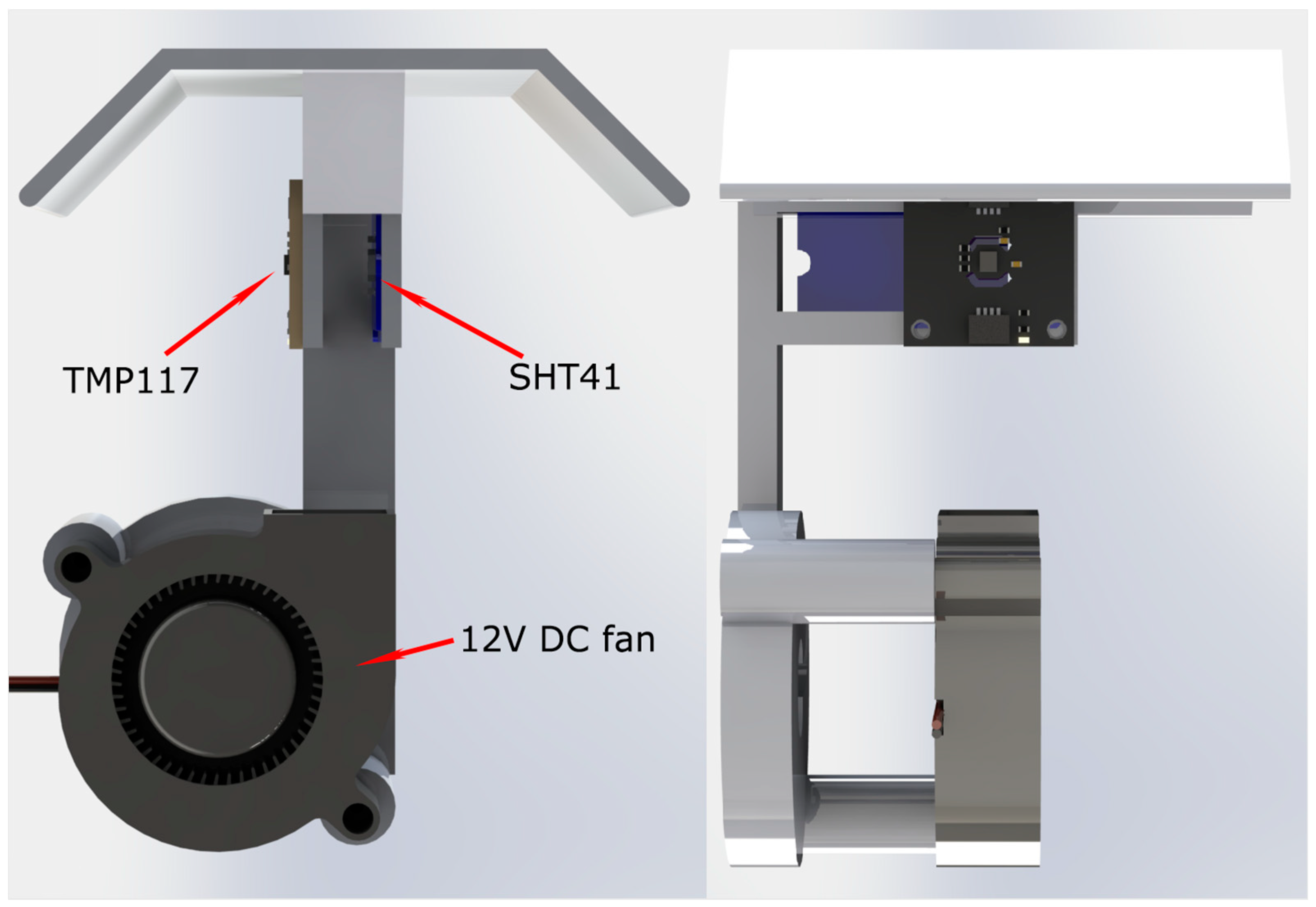Only a handful of studies [15,24,25] have used sensors of higher than 0.5 °C accuracy, which does not meet the WMO minimum characteristic requirement [27]. The TMP117 sensor used in this study was selected due to its high accuracy of 0.1 °C. A notable data processing method was described by Chang et al. [13] of using the temperature reading and the rate of change in the reading to predict the actual ambient temperature. This method was also adopted in our work and improved the accuracy of the data collected by reducing the inertial errors.

Vertical measurement of atmospheric parameters is pivotal for enhancing our comprehension of atmospheric stability, pollutant distribution, urban heat island formation, and precise weather predictions. Traditional methods, such as weather balloons, have been indispensable but are challenged by limitations like cost, environmental impact, and sparse data. UASs emerged as a promising alternative, offering cost-effectiveness, mobility, and reusability for in situ probing. Addressing challenges like measurement resolution while harnessing UASs’ versatile range of motion, can herald a new era of atmospheric research, leading to more accurate forecasting and better environmental risk management.

The aim of this work is to explore the efficacy and accuracy of UASs in capturing vertical atmospheric profiles, particularly focusing on temperature gradients, and comparing their performance with traditional methods like weather balloons. This article focuses on the analysis of the lower boundary layer, a relatively underexplored area in meteorology, which also conforms to airspace regulations. Heights ranging from 5 to 120 m have been selected for examination.

2. Materials and Methods

2.1. Geographical Location and Background

Our experimental investigations took place in Vilnius, the capital of Lithuania, a region predominantly characterized by expansive plains and lowlands, leading to a relatively flat terrain. This flat terrain predisposes the region to temperature inversions, especially during calm and clear nights. Temperature inversion is a phenomenon where a layer of cooler air near the ground is trapped by a layer of warmer air above. In urban environments, this can lead to trapping of pollutants, causing smog and deteriorated air quality. Such inversions become more pronounced in flat terrains like Vilnius, as the absence of hills or mountains prevents the vertical mixing of air layers. Additionally, flat areas, compared to hilly terrains, usually exhibit a more consistent humidity distribution. Without inversions, flat terrains display predictable and uniform vertical temperatures and humidity profiles. This consistency offers an ideal backdrop for evaluating inertial parameters, reducing the experimental variables. Given the urban context of our study, a multirotor UAS drone is best suited to investigating the vertical profiles. Traditional horizontal flights can pose challenges, especially when landing in constrained spaces.

2.2. Hardware Used

2.2.1. Thermometer Selection

In the initial phase, the temperature sensors were subjected to a comparative analysis with data obtained from a local meteorological station. Various types of sensors, such as a platinum RTD, DHT22, BMP280, and TMP117, were utilized for this purpose. These sensors were connected to a single board, which facilitated the logging of all recorded measurements onto a memory card. The instruments were strategically housed within a ventilated and sun-shielded enclosure, positioned a few meters away from the meteorological station at an identical height.

Throughout the course of the experiment, which spanned 16 h, the ambient temperature exhibited fluctuations within the range of 2 to 13 °C. For analysis, the data points were resampled to the frequency of the reference station ($\frac{1}{5} \mathrm{H}\mathrm{z}$) and an offset was applied such that the RMSE between the data from the meteorological station and the sensors being tested was at a minimum. The smallest error was recorded on the TMP117 sensor with the RMSE of the unadjusted dataset being 0.12 °C and 0.10 °C when a 0.06 °C offset was applied. This is consistent with the accuracy figures provided by the manufacturer. Extensive testing allowed us to choose the sensor with the lowest approximated absolute error.

Furthermore, the thermal mass of the sensor played a pivotal role in the context of this experiment. The dimensions of the TMP 117 circuit board are significantly compact; also, a relatively high degree of exposure of the sensor to the surrounding environment is prominent. These two critical factors suggest that the thermometer may exhibit superior responsiveness to fluctuations in the environment, resulting in a reduced time constant for its thermal response.

2.2.2. Chosen Final Configuration

For the purpose of conducting the experiment, a thermometer rig consisting of a TMP117 and SHT41—a high-accuracy relative humidity sensor—was utilized. These instruments were securely enclosed within sun-shielded housing, as depicted in Figure 1. The fan-ventilated rig was affixed onto the DJI M300 drone leg as illustrated in Figure 2a.

As a reference, on the other leg of the drone, a Vaisala radiosonde RS41 was attached. It is a state-of-the-art-powered instrument that can be launched into the atmosphere via a balloon and measures various atmospheric parameters such as temperature, humidity, wind speed, and direction. The RS41 features advanced sensors and radiosonde technology that provide high accuracy and reliability for data collection. The temperature repeatability in the calibration accuracy is ±0.1 °C; see more details in

Table 1. TMP117 and SHT41 sensor specification.

Sensor (Parameter)	Accuracy (Range)	Resolution	Sampling Period, s	Time Constant, s
TMP117 (temperature)	±0.1 (−20–50) °C	0.0078 °C	0.06	20
SHT41 (humidity)	±2.5 (0–90)%	0.01%	0.06	20
RS41 (temperature)	±0.1 (−90–60) °C	0.1 °C	1	0.5
RS41 (humidity)	±2 (0–100)%	0.1%	1	0.3

. During testing below a 16 km altitude, it was found that the temperature accuracy was ±0.3 °C, and the humidity ±3% [28]. Lee et al. [29] have used simulations to determine the error caused by solar irradiation on the Vaisala RS41 radiosonde temperature sensor to be 0.119 °C. The sensor response times are stated to be 0.5 s for temperature and 0.3 s for relative humidity at 1000 hPa pressure and 6 m/s airflow. The radiosonde is also equipped with global positioning system (GPS) technology that enables precise location tracking and data transmission capability via radio antenna. The RS41 radiosonde gathers data at a comparable accuracy to the TMP117 and SHT41 sensors; however, the resolution and sample rate were significantly lacking in contrast to other equipment used. The chosen RS41 sensor specifications are summarized in Table 1. Its mounting is illustrated in Figure 2b.

Additionally, pressure data from a BMP280 sensor with a relative accuracy of ±0,12 hPa (~1 m pressure altitude) and resolution of 0.01 hPa was used to determine pressure-altitude [16].

According to the WMO [27], the minimum thermometer characteristic requirement is <0.3 °K of error. The time constant—the time required by the thermometer to register 63.2% of a step change in air temperature assuming that the sensor has a first-order response to changes in the measurand (namely, the rate of change in the measurement is proportional to the difference between the measurement and the measurand)—should be 20 s. An achievable observing accuracy for the relative humidity (RH) measurements is 3–5% and the target uncertainty stated as two standard deviations is 5% for medium and 1% for high RH. The sensor time constant should be 40 s.

A 3D-printed sun shield and ventilation device, fabricated from white polylactic acid (PLA), was developed with the primary objective of reducing thermal inertia, enhancing ventilation around the thermometers, and shielding against solar radiation during experiments. The prototype’s schematic is presented in Figure 1.

The utilization of white PLA was an effective measure to mitigate material heating due to solar radiation. The design incorporates minimal plastic around the thermometers to reduce thermal inertia and unimpeded airflow to increase the thermometers’ exposure to the surrounding airflow. This was helpful as inertia reduced to adequate levels compared to in previous housing prototypes.

To prevent pressure variations due to dynamic pressure from the downwash affecting the height data, the BMP280 barometer was strategically placed away from the propellers, below the drone, in a box, isolated from the surrounding air currents together with an Arduino Nano microprocessor, to which all sensors were linked. A real-time clock (RTC) module (2 ppm accuracy) was employed to allocate timestamps, and the data were stored in an SD card at a frequency of 50 Hz.

2.2.3. Sensor Reaction Time Determination

The reaction time of the temperature sensors was measured by rapidly changing the environment. During the response time testing of the thermometers, calm, enclosed, and static environments were chosen to increase the consistency between the results obtained. After three such measurements, the time required to reach a 63.2% step change in ambient temperature was averaged to 20.7 s, although the sensor readings did not always closely follow the first-order response to changes in the measurand (Newton’s cooling law) when approaching ambient temperature. Examples of the sensors’ response can be seen in Figure 3.

From these experiments, it was possible to determine how rapid the response of thermometer rig was (shown in Figure 1). After the temperature response time of this rig was determined, it was possible to estimate real environment temperature values using the temperature gradient. This gradient can indicate how far away the environment temperature is. It enables extrapolating the environment temperature $T_e$ from the change in temperature over time t.

$$T_e=T\left(t\right)+\frac{d\left(T\right)}{dt}\times \frac{1}{r} ,$$

(1)

where r is the reaction time constant depending on the intrinsic thermometer properties and also its surroundings, such as airflow, thermal mass, etc. T(t) is the temperature as a function of time. $\frac{d\left(T\right)}{dt}$ was computed by subtracting adjacent temperature readings; however, due to small fluctuations in temperature over a small time scale caused by real-life uncertainties, it was chosen to determine $\frac{d\left(T\right)}{dt}$ by subtracting temperature readings spaced out by several seconds, dt. An r of 20 s and 40 s of dt were chosen as this was best to the approximate values. These values are later used in experimentation Section 3.2, which approximates to the lowest mean square error compared to the settled temperature.

2.2.4. Hardware Limitations

The selection of the DJI M300 drone for this study was based on careful consideration of its pertinent specifications, notably its substantial carrying capacity of 2.7 kg and reasonably extended endurance of 50 min (as per reference [21]). With the DJI M300 drone configured in this particular manner, it is plausible to achieve altitudes of up to 1500 m within a total flight time of 50 min. It is essential to emphasize that our assumptions for this study encompass the use of a consistent ascent and descent speed of 1 m per second (1 m/s), as well as the presumption of an optimal battery performance without the need for active heating. While it is recognized that various drone models may exhibit varying capabilities, the DJI M300 drone selected for this research unequivocally proved to be highly adequate and well suited to the specific purpose of conducting measurements at lower altitudes.

While it is possible to enhance the rate of climb and descent to 6 m/s for ascent and 5 m/s for descent, especially with this specific drone, which would enable even greater altitudes, it is essential to acknowledge that such maneuvers may adversely affect the accuracy of temperature data acquisition. In this research, the primary objective is to ensure the utmost accuracy of the collected data; thus, the pursuit of higher altitudes is not a priority. Additionally, it is important to recognize that when the time intervals between ascent and descent at the same altitude are substantial, it can significantly reduce the temporal resolution, which is not conducive to our research goals.

Furthermore, it should be noted that the accuracy of temperature sensing using a TMP 117 and SHT 41 may decrease slightly at very high altitudes. In accordance with the International Standard Atmosphere (ISA), temperatures typically start at 15 °C at sea level and progressively decrease with height in the troposphere, ultimately reaching an average of −56.5 °C. Given that the hardware (TMP 117 and DJI M300) used in this experiment is capable of operating at highest accuracy in temperatures ranging −20 °C to 50 °C, and later decreasing in accuracy to ± 0.25 C when operating between −55 °C and 125 °C, the accuracy may therefore degrade in extremely cold weather conditions at high altitude. Similarly, the humidity sensor SHT 41 is designed to be most accurate up to 90% water saturation. These considerations informed our choice of instrumentation for this study.

2.3. Data Processing

The data from the TMP117 and SHT41 sensors were logged to an SD card in case of sensor assembly using an Arduino Nano and a card reader in Comma-Separated Values (CSV) format and moved to a Windows computer after every flight. Software-defined radio (SDR) equipment (a universal serial bus receiver, a Windows computer, and HD SDR software v2.80 [30]) was used to capture the radiosonde data. The radio signal was decoded using an RS41 decoder by RS41 Tracker v1.5 [31]. The logged data were exported to a CSV file for processing.

The logs were accessed using Jupyter Notebook—an interactive computing environment, running a Python 3.9.13 kernel. The NumPy 1.23.5, pandas 1.4.4, and Matplotlib 3.7.1 libraries were used.

To synchronize the data from the two sources, an RTC was used with an Arduino logger to provide timestamps for each measurement iteration. The timestamps of the radiosonde data were derived by using a GPS. Due to the nature of manually setting the RTC, an offset of several seconds was unavoidable. This was later corrected by synchronizing the radiosonde and sensor assembly altitude peaks.

Since the temperature logging device samples the data at fixed time intervals (1 s), the altitude intervals can be variable depending on the vertical speed of the vehicle. Furthermore, the data points are sampled at a different altitude while ascending and descending. To make data processing in relation to altitude possible, some interpolation is necessary. According to Hemingway et al. [14], vertical sampling scales of approximately 3 m for temperature and 1.5–2 m for relative humidity were sufficient to capture the spatial structure of these parameters under the conditions tested. Therefore, the data from the measurement devices were resampled in relation to the altitude every meter.

2.4. Experiment Setup

Initially, the sensors were allowed to acclimate to the environmental conditions at ground level while the drone remained stationary. A deliberate decision was made to execute a gradual ascent at a rate of 1 m/s, followed by an equivalent descent. This approach aimed to optimize the duration during which the thermometers were exposed to temperature and humidity conditions at a specific altitude, thereby minimizing potential hysteresis errors.

To facilitate a consistent vertical speed during the ascent, an automated mission was designed. The midpoint of this mission was established at an altitude of 120 m above ground level, a value determined by the authorities for non-specialized drone operations.

Upon reaching the peak altitude, the drone promptly initiated its descent without waiting for the sensors to stabilize. Both the beginning and ending points of the flight were situated at ground level. The sequence of the flight, including the ascent and descent, is outlined in Figure 4.

In Figure 4, the complete course of a single mission is depicted. The blue line in the graph corresponds to the pressure altitude, which was measured using a BMP 280 sensor located within a ventilated enclosure, carefully protected from the disturbance caused by the propeller airflow. The temperature data were obtained from a TMP117 sensor that was positioned on the rig depicted in Figure 1.

3. Results

3.1. Number of Experiments and Their Validity in the Study

The main objective of this study was to compare the capabilities of a radiosonde RS41’s temperature gradient with a low-cost TMP117’s. In order to acquire as accurate results as possible, multiple flights were undertaken. A total of 28 flights from 26 May to 15 June 2023 between 7:00 and 15:00 UTC took place. Out of those 28 flights, 16 were selected as adequate to analyze. Flights no. 1, 7, and 26 had incomplete radiosonde datasets (failed to properly log, signal loss, data corruption, and battery problems), flights no. 2, 9, 12, and 27 landed on different temperature surfaces (discarded to lower the amount of different error sources), flights no. 10, 25, and 28 had too much sun exposure, and flight no. 19 had an incorrect sequence (procedure differed from all other flights). All flights were analyzed and used for the development of processing improvements, but only full flights with no extremities in environmental or flight conditions were used for further sections of this article and its results (

Table 2. List of experimental flights conducted with TMP117 and SHT41 sensors for results and analysis.

Flight Start Date & Time		Flight Number
20 May 2023	12:30:00	4
30 May 2023	9:30:00	5
30 May 2023	13:30:00	6
31 May 2023	12:30:00	8
02 June 2023	8:00:00	11
05 June 2023	8:00:00	13
05 June 2023	14:30:00	14
06 June 2023	7:30:00	15
06 June 2023	11:00:00	16
06 June 2023	13:30:00	17
07 June 2023	8:30:00	18
08 June 2023	8:30:00	20
08 June 2023	14:30:00	21
09 June 2023	6:30:00	22
12 June 2023	8:00:00	23
12 June 2023	12:30:00	24

).

3.2. Data Evaluation Method Illustration from One of the Flights

For the illustration of values, the first valid flight was chosen to showcase, define, and compare algorithms and their results in evaluating the boundary layer’s temperature values. When measuring the TMP117 values, both the climb and descent values were evaluated. These values almost never matched between the ascent and descent; therefore, some interpretation was needed. As mentioned in the introduction, this is a hysteresis problem. More details about this problem can be seen in Figure 5 depicting how temperature is mapped out in relation to height over time.

The chart on the right displays the altitude of the drone during one of the flights. The colors represent different time intervals under examination, with dark blue indicating the start of the climb, and yellow indicating the descent and landing phase. Each data point on the chart represents a single recording. The relatively high data logging rate results in the appearance of a nearly continuous line.

As the mission was automated, measures were taken to maintain a constant speed without fluctuations during both the ascent and descent phases.

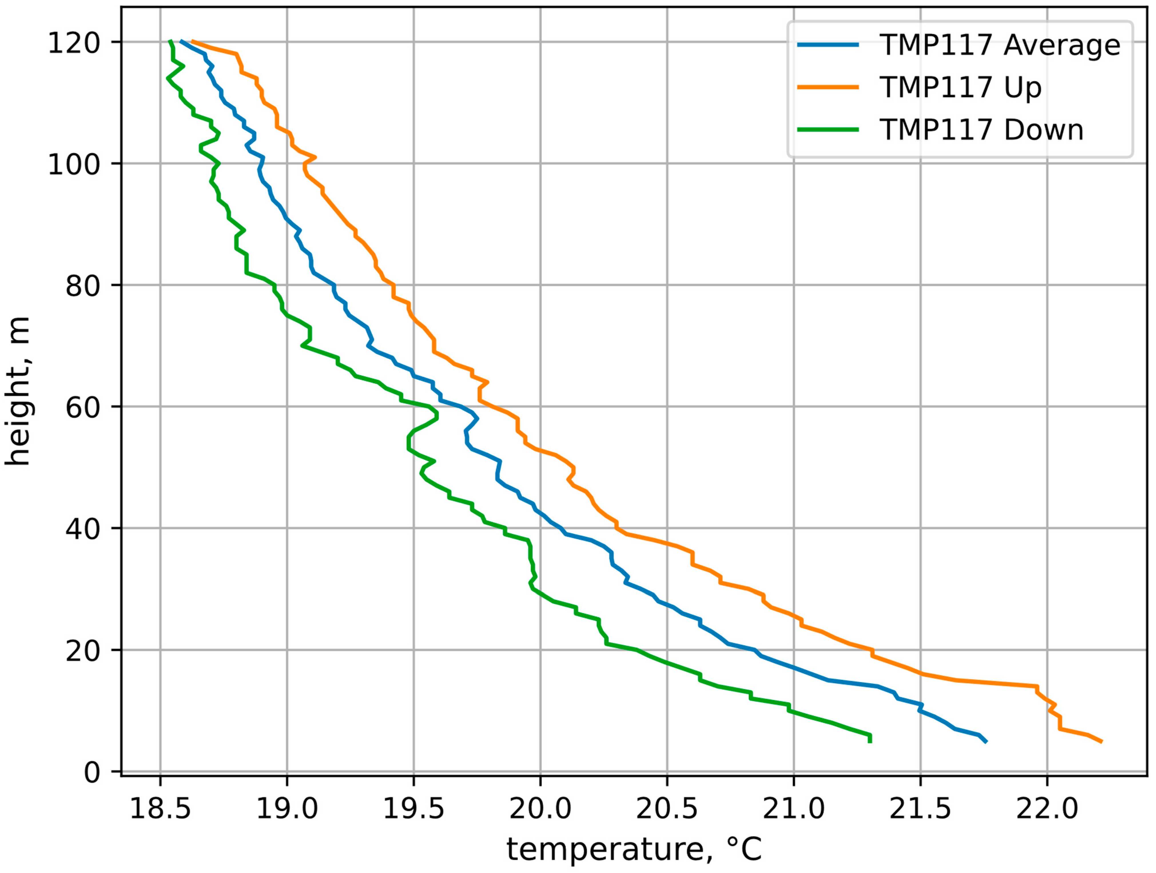
In Figure 5a, we observe the raw TMP117 sensor readings throughout the ascent and descent. Fluctuations in these readings are evident, attributed to uncertainties in weather conditions, such as wind patterns, air mixing, and other external factors. Additionally, it is noticeable that the initial temperatures at the beginning of the experiment appear to be slightly warmer than those recorded toward the end of the experiment. This pattern is seen across all the experimentation carried out in this study. The cause of this pattern is a hysteresis phenomenon. Since the values do not match when climbing and descending within the TMP117 sensor data, averaging was used; an example of the averaging of these values can be seen in Figure 6.

Figure 6 depicts the identical ascent and descent profile shown in Figure 5. However, in this representation, the average values for both the climb and descent phases are presented, while certain low-altitude data points (specifically those at 5 m above the ground and below) have been excluded. These excluded data points pertain to instances where the temperature was reported to stabilize at the same height, and their omission serves to prevent any potential confusion.

The main goal of this study was to examine errors in these measurements and evaluate the most probable temperature values at each height. To achieve this, the temperature gradient was evaluated in the following manners:

• Using the average values of the TMP117 from climb and descent.
• Using time-shifted TMP117 values and then averaging them.
• Using Newton’s law of cooling to predict appropriate readings and then averaging the results from the climb and descent.

The results of each gradient measurement methodology were crosschecked with the RS41 data, which is considered a gold standard.

A fixed time shift between the recorded altitudes and temperature readings was suggested by the authors. By shifting the temperature data back in time, we see closer correlation of temperatures at the same altitude while ascending and descending. From each ascent and descent, we find a time when the drone is at the maximum altitude, the peak. We also find the peak of our temperature profile; however, it is recorded later in time. The time of the temperature readings is shifted backward to match the altitude peak. The resulting graph in time can be seen in Figure 7. The averaged climb and descent values of the time shifts are illustrated in Figure 8.

An additional technique employed in the study was Newton’s law of cooling. The formulas and methodologies outlined in Section 2.2.3 were applied to estimate the most probable ambient temperature. The variations in temperature can be observed in both Figure 7 and Figure 8, presented concurrently with the time shift and raw data.

The graph displays raw temperature values represented in blue, while time-shifted values are depicted in green. The time-shifted values remain identical to the blue values but have been adjusted to align with the peak of the climb, which occurred approximately 3 min and 14 s after the start of the experiment. The yellow lines correspond to Newton’s law of cooling, which responds to changes in the raw temperature values. Observationally, during the initial phase of ascent, the temperature does not achieve its minimum point at the peak, due to the sensor response time and a prompt descent after the climb. Newton’s law of cooling is anticipated to counteract this trend by approximating lower values at the point of measurement. The utilization of the time shift technique is not able to accomplish this objective.

Both of these techniques were thoroughly tested, and the averaged values of both the ascent and descent phases were selected for further analysis. A sample dataset of the vertical boundary layer temperatures can be observed in Figure 8.

All methods exhibit a considerable degree of correlation with each other. However, it is essential to note that this analysis is based on data from a single flight sample, making further flights assessing the reliability of these methods more comprehensively a necessity.

As a reference, the radiosonde RS41 data was collected to crosscheck its values with the TMP117 data. The raw data values from the RS41 exhibited substantial fluctuations. To address these challenges, post-processing techniques, such as Savitzky–Golay and iterative filtering for smoothing, were employed to estimate the true atmospheric conditions. Savitzky–Golay filtering uses each outlier filtered and its neighboring temperature readings in a time sequence. Specifically, five neighboring temperature readings are utilized, and a polynomial line is fitted to this set. The resultant central value of this polynomial line represents the smoothed value sought in estimation. The selection of five neighboring readings stemmed from empirical experimentation, which revealed that this choice effectively smoothed the data, yielding a relatively uniform vertical profile line while retaining the essential dataset details without excessive smoothing. An iterative filter smoothing technique was used to improve the uniformity of a gradient (T) with respect to height (h) by iteratively adjusting the values to minimize variations. Firstly, the average values from the ascent and descent were taken and their averages were later smoothed out with an iterative filtering method. The iteration processes were applied four times as this made the data relatively uniform across the entire examined height. The improved approximations resulting from these smoothing methods are illustrated in Figure 9.

Following the data collection process and its requisite preprocessing, the decision was made to employ the linear regression technique for result comparison. This method was deemed suitable due to the absence of any gradient inversions or non-standard atmospheric conditions among the examined gradients, as verified via careful assessment. The application of linear regression encompassed the untreated radiosonde data, serving as a basis for comparison against the TMP117 data.

Moreover, the linear regression methodology was also cross-validated with the TMP117 data, employing various processing techniques, such as raw, shifted, and Newton’s law of cooling methodologies. An illustrative depiction of how linear regression interpolates data from the raw dataset is presented in Figure 10.

Evident temporal variations in temperature are discernible within the vertical profile. The substantial amplitude of temperature fluctuations produces overlapping outcomes during the ascent and descent. Consequently, the decision was made to exclusively consider values derived from the ascent phase during the assessment of the RS41.

Notably, the TMP117 sensor presents a notably more stable temperature reading across the vertical profile as contrasted with the radiosonde data.

3.3. Comparisons of Gradients across Flights Employing All the Techniques Described

Once a robust experimental approach was defined, outlining the execution and specifying the algorithms for result interpretation, gradient values were computed for each valid experiment. A total of 16 sets of experimental data were assessed.

Table 3. TMP117 and RS41 gradient comparisons of °C change per 100 m ascent.

Flight Number:		#5	#17	#21	Average
TMP117	Averaged	−1.64	−1.63	−1.17	−1.72
	Shifted	−2.13	−1.37	−1.15	−1.76
	Newton’s law	−1.86	−1.09	−1.25	−1.68
RS41	Raw data	−1.87	−0.63	−1.58	−1.53
	Savitzky–Golay filter	−1.94	−0.64	−1.54	−1.50
	Iterative filter	−1.88	−0.62	−1.53	−1.49

presents a collection of the sample gradients derived from various datasets: TMP117 raw data, shifted data, and data corrected using Newton’s law, along with the RS41 raw data, data processed using a Savitzky–Golay filter, and data treated with an iterative filter.

Flight numbers 5 and 17 were selected to illustrate how the shifting time of the TMP117 can influence the calculation of temperature gradients, potentially resulting in either amplified or diminished gradient values. Additionally, flight #5 highlights the remarkable accuracy of Newton’s law of cooling, showing a robust correlation with the RS41 values. Nonetheless, it is worth noting that Newton’s law of cooling is not infallible, as evidenced by the deviations observed in flights #17 and #21. On average, the data derived from Newton’s law of cooling appear to exhibit the highest degree of consistency with the RS41 radiosonde measurements. The approximate deviation of the TMP117 with Newton’s law of cooling post-processing is only approximately 0.2 °C.

Furthermore, the TMP117 dataset was examined and its RSME was calculated from all 16 flights made that were deemed to be valid and from which correct non-corrupted data was acquired.

Table 4. TMP117 RMSE per 100 m gradient when compared to RS41.

Compared against	TMP117 Interpretation	RMSE
RS41 Savitzky–Golay filter	Raw	0.454 °C
	Shifted	0.398 °C
	Newton’s law	0.290 °C
RS41 Iterative filter	Raw	0.452 °C
	Shifted	0.411 °C
	Newton’s law	0.297 °C

depicts the TMP117 RMSE when comparing it to the RS41’s with Savitzky–Golay filtering and iterative filtering. The raw, shifted, and Newton’s law values for the TMP117 are compared separately.

Upon scrutinizing the data collected from the TMP117 sensor, it becomes evident that the unprocessed data demonstrate the weakest correlation with the RS41 measurements, registering only 0.45 °C. The shifting technique offers a slight improvement, reducing the RMSE to around 0.4 °C. In contrast, Newton’s law of cooling yields the most favorable outcome, showcasing the lowest RMSE when compared to the RS41 reference measurements, with a reduction of down to 0.290 °C.

Later in this study, differences in temperature across entire the flight altitude was analyzed. From each flight, the Δ$\mathrm{T}$ between the TMP117 and RS41 was taken for each altitude. The results from all 16 valid flights are represented in Figure 11.

In Figure 11a, the analysis of the raw temperature differential derived from the RS41 data reveals a notable concurrence of temperature readings at ground level. However, subtle deviations emerge as altitudes increase, indicating a slightly positive Δ$\mathrm{T}$ at a low altitude, while at higher altitudes, a minor negative bias is observed. The subsequent portrayal of the shifted temperature data in Figure 11b elucidates a resemblance to the aforementioned raw temperature data pattern, albeit with a slightly augmented dispersion of data points across varying altitudinal levels. The dispersion of shifted data exhibits a substantial increase at 35 m and a minor rise at 85 m when contrasted with both the unprocessed data and Newton’s law of cooling data. The latter demonstrates a relatively consistent dispersion throughout the entirety of the flight altitude. A slight reduction in dispersion is noticeable at the peak of the ascent across all datasets.

The utilization of Newton’s law of cooling, as presented in Figure 11c, manifests a discernible inclination to exhibit a marginal underestimation of temperature measurements across the altitude spectrum. This inclination is further underscored by a propensity to register comparatively lower temperatures at the top of a climb. Remarkably, both the raw temperature data and the data processed through the application of Newton’s law of cooling display a convergence toward a narrower data spread as the altitude ascends during the height assessment.

4. Discussion

Unmanned aerial systems (UASs) have been demonstrated as a promising platform for atmospheric temperature profiling. The results of this study show that UAS-based temperature measurements can provide accurate and reliable data, with comparable performance to conventional methods such as radiosondes. Moreover, UASs offer several advantages over these traditional techniques, including lower cost, greater mobility, and higher spatial and temporal resolution.

In this study, specific data processing techniques were applied to improve the accuracy and consistency of the temperature readings obtained from the UAS. These techniques included smoothing methodologies such as the Savitzky–Golay filter, iterative smoothing, time shift, and Newton’s law of cooling. By applying these methods, patterns between different methodologies and sensors were identified, and the accuracy of the temperature profiles obtained from the UAS was improved. An accuracy achievement of 0.16 ± 0.014 °C with 95% confidence when applying Newton’s law of cooling in comparison to a radiosonde RS41’s data concluded that this setup exceeds the WMO “breakthrough” requirement for the accuracy of measurements used for atmospheric climate forecasting and monitoring. This is compared to the results from an extensive study by Hervo et al. during which the UAS measurements were compared to a balloon-tethered radiosonde’s data, resulting in 0.68 °C accuracy. This campaign, however, did not provide results up to 500 m of height, because of a high positive bias from the meteorological UAS. Our study demonstrates high accuracy and resolution at the lowest atmospheric surface layer, at which the parameter gradients tend to be the strongest.

Other articles have analyzed temperature inertia and errors associated with this phenomenon and evaluated the most probable temperature values at each height with 0.2 °C accuracy [13]. In our study, a more detailed look was taken into temperature gradient, extracted from time-shifted TMP117 values and the application of Newton’s law of cooling to predict appropriate readings and then average the results from the climb and descent. The results of our work demonstrate the improvement in accuracy of the vertical temperature profiles and suggest that UASs, with further refinements, could revolutionize atmospheric data collection methodologies.

Despite the challenges associated with evaluating temperature readings obtained from UASs, UAS-based atmospheric measurements offer unique research opportunities that are not possible when using conventional methods. For example, UASs can be used to study vertical parameter gradients, which are important factors in weather forecasting, air quality monitoring, and small-scale climate modeling. The discussed measurement and data processing methods may be used for affordable, high-precision atmospheric probing. Future work may involve the measurement of vertical and horizontal temperature profiles in urban environments, for example, mapping urban heat islands and temperature inversions. To increase the dimensionality of the measurements, rows or grids of drones could be deployed in unison. Enhancements in temperature data analysis can be pursued through the incorporation of advanced methodologies, such as autopilot rate control during ascent and descent, which relies on the detection of temperature gradient variations. This approach enables the mitigation of abrupt temperature gradient fluctuations causing inaccuracies, thereby preserving high precision and optimizing flight duration. To further augment accuracy, algorithms integrating considerations for solar exposure, airflow patterns surrounding sensors, and various extraneous factors can be devised and integrated using artificial intelligence (AI) models. This would help identify natural or manmade sources of temperature anomalies which have significant implications for public health and energy consumption.

A limiting factor for this research campaign was the 120 m height limit for open category drone operations imposed by the authorities in the European Union. Despite this, we were able to capture the air temperature gradient with great precision. Due to the number of flights conducted, it was not feasible to assess the reliability of this system for professional operations; however, most problems encountered were related to the radiosonde (loss of signal) or caused by human error (incorrect measurement procedures).

In conclusion, this study highlights the potential of UASs as a valuable tool for atmospheric temperature profiling by demonstrating their high accuracy and resolution in the surface layer of the atmosphere. Further research is needed to address the technical and methodological challenges associated with UAS-based measurements, and to explore the full range of research opportunities enabled by this emerging technology.