Abstract
The temporal monitoring of indicator plant species in high nature value grassland is crucial for nature conservation. However, traditional monitoring approaches are resource-intensive, straining limited funds and personnel. In this study, we demonstrate the capabilities of a repeated drone-based plant count for monitoring the population development of an indicator plant species (Dactylorhiza majalis (DM)) to address such challenges. We utilized multispectral very high-spatial-resolution drone data from two consecutive flowering seasons for exploiting a Random Forest- and a Neural Network-based remote sensing plant count (RSPC) approach. In comparison to in situ data, Random Forest-based RSPC achieved a better performance than Neural Network-based RSPC. We observed an R² of 0.8 and 0.63 and a RMSE of 8.5 and 11.4 DM individuals/m², respectively. The accuracies indicate a comparable performance to conventional plant count surveys. In a change detection setup, we assessed the population development of DM and observed an overall decline in DM individuals in the study site. Regions with an increasing DM count were small and the increase relatively low in magnitude. Additionally, we documented the success of a manual seed transfer of DM to a previously uninhabited area within our study site. We conclude that repeated drone surveys are indeed suitable to monitor the population development of indicator plant species with a spectrally prominent flower color. They provide a unique spatio-temporal perspective to aid practical nature conservation and document conservation efforts.
1. Introduction
High nature value grasslands are ecologically diverse and play a vital role in the conservation of endangered plant [1,2] and animal species [3,4]. Nevertheless, many European high nature value grasslands are threatened by human activities [5,6] and/or climate change [7,8]. Recognizing the severity of the situation, the European Union (EU) has devised legal instruments and long-term conservation strategies, such as the Habitat Directive [9], Bird Directive [10] and the NATURA 2000 network. Their goal is to protect, conserve, and restore ecosystems across the EU. The EU member states translated these overarching goals to site-specific conservation objectives, necessitating regular monitoring to assess the progress towards these goals. A prevalent approach involves recurring monitoring of indicator species [11] that serve as proxies for habitat integrity [12]. They are generally associated with specific environmental conditions, wherefore a change in the population of such species indicates changing habitat conditions.
Plant species from the family Orchidaceae serve as valuable indicator species for a variety of habitats due to their diversity, high habitat specificity and sensitivity to environmental changes [13,14]. Dactylorhiza majalis (DM), also known as broad-leaved marsh orchid, particularly stands out as an indicator species for wet and nutrient-poor grassland habitats in Central Europe [15]. The species has experienced a notable decline over the past two decades [16,17], which has prompted several Central European countries, such as Germany [18], the Czech Republic [19] and Switzerland [20], to categorize DM as an endangered species. The widespread decline is attributed to habitat changes due to the intensification of agriculture, drainage, and the abandonment of land use, as well as afforestation [16]. To counteract further population decline, conservationists implement site-specific conservation measures to retain or restore favorable habitat conditions, such as late mowing in mid-July (after the flowering phase) or scrub removal. However, the effectiveness of these efforts remains unclear, for which reason the spatially accurate monitoring of DM becomes a necessity.
Traditionally, expert monitoring programs involve repeated labor-intensive field campaigns with manual plant counting [21] or population size estimation based on limited samples [22]. However, these approaches have methodological limitations. With the increasing size and inaccessibility of the study site, data acquisition becomes impractical and less accurate. In the last decades, some expert monitoring programs were supplemented by volunteer workforce (e.g., [23]). And although studies reported positive results [24,25,26], such monitoring program designs introduce additional dependencies for successful data acquisition, i.e., the willingness of a sufficiently large volunteer group to participate. Additionally, the effect of non-expert acquired data on the result quality often remains unquantified [27].
Remote sensing (RS) techniques offer a solution to cope with the scaling problems inherent to traditional mapping approaches [28]. Several studies have shown that spectrally prominent flower colors can be used to identify key plant species [29,30,31,32,33,34,35,36]. This identification is possible because these flower colors generally show distinct spectral responses compared to green vegetation [37,38]. In the last few decades, satellite Earth Observation investigations have consistently highlighted the potential of machine learning techniques for image classification. However, the history of machine learning for drone-based image classification is relatively recent, dating back to the early 2000s [39]. This domain has seen rapid development and advancement since, as a result of the convergence of critical technologies such as drone hardware and machine learning algorithms. Recent investigations have reported promising results in counting plant individuals with drone-based RS data using different image analysis techniques, such as Random Forest (RF) classification [36] and deep learning approaches [40,41].
In one of our previous studies, we proposed an RS-based alternative for monitoring plant species with a spectrally prominent magenta-colored flower, using DM as our target species [36]. However, our previous analysis only looked at the DM population for a single point in time. In this study, we extended the RS-based DM monitoring by the temporal dimension using a new drone dataset acquired in the consecutive flowering season. By leveraging the temporal dimension and paying special attention to data and processing consistency, we assessed the DM population development (loss or gain) in a spatially comprehensive manner. Additionally, we investigated the optimization potential of our previous approach. We compared the performance of a Neural Network (NN) classifier to RF, which was previously proposed in [36]. In summary, our study’s goals are as follows:
- 1.
- Show the potential of an RS-based analysis to assess the population development of an indicator species with a spectrally prominent flower.
- 2.
- Improve the understanding of RSPC, based on drone data, in comparison to an in situ plant count field survey.
- 3.
- Extend the RSPC methodology proposed by [36] by the temporal dimension and investigate its optimization potentials.
2. Materials
2.1. Study Site
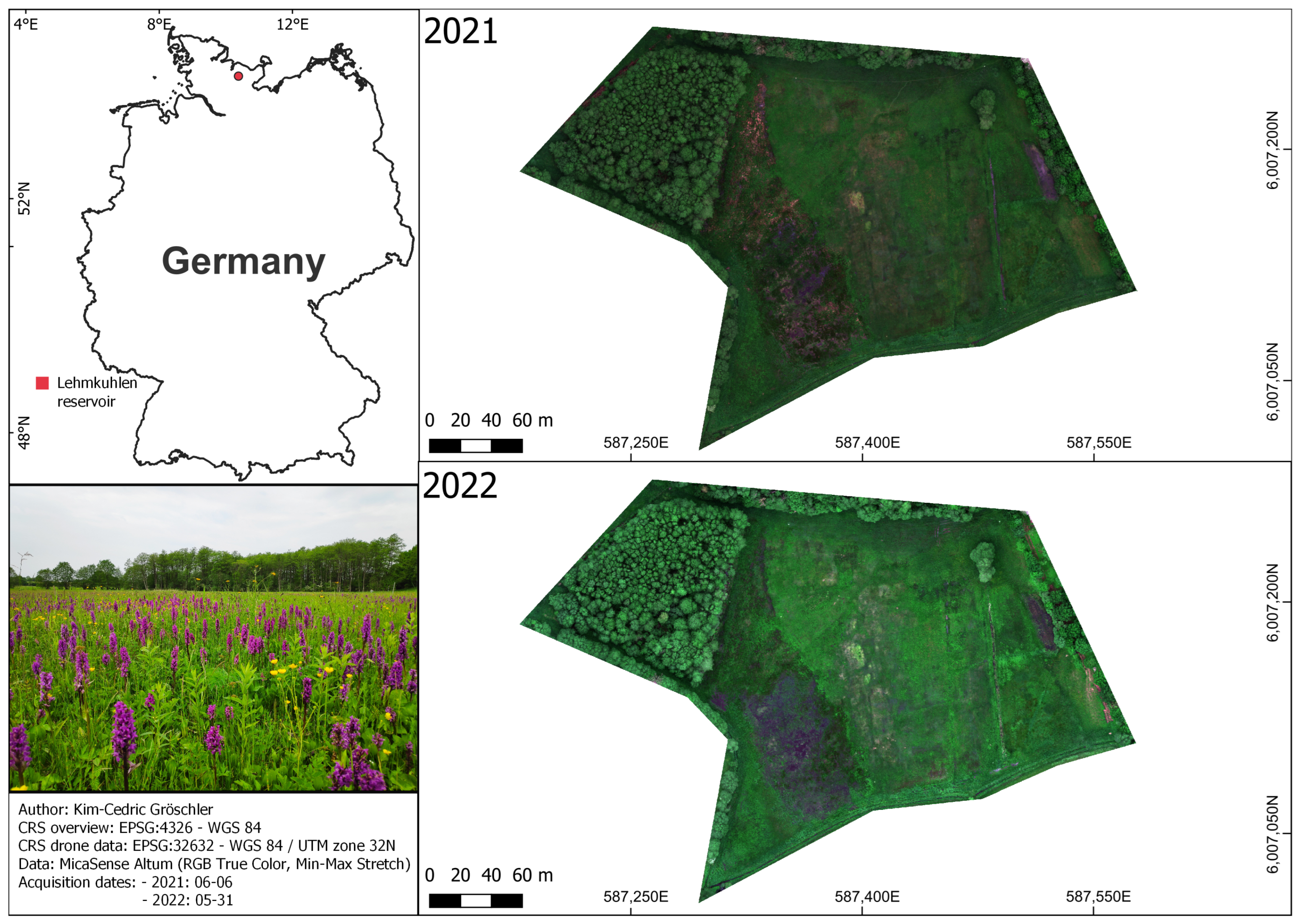
We acquired the data for this study in the Lehmkuhlen reservoir (Figure 1), Schleswig-Holstein, Germany, where conservationists reported the largest statewide DM population [42]. The Lehmkuhlen reservoir is an alkaline, nutrient-poor fen which developed during the Weichselian ice age [43]. Over an area of 0.29 km², conservationists reported 60 endangered plant species (including DM) in the study site [43]. Due to its ecological importance, it is protected by the European Habitat Directive (NATURA 2000 codes: FFH 7230—alkaline fens and FFH 7140—transition mires) and managed by conservationists to retain favorable habitat conditions.
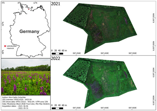
Figure 1.
Overview of the study site during the investigation years 2021 and 2022. The photograph illustrates the abundance of Dactylorhiza majalis during data acquisition.
2.2. Drone Data
We conducted drone flights during two consecutive flowering seasons of DM on 6 June 2021 and 31 May 2022. During these periods, local conservationists verified that no other plant species with magenta-colored flowers blossomed in our study site. The commissioned company used a Wingtra One drone equipped with a MicaSense Altum sensor for both acquisition campaigns. The sensor captured multispectral data with bands in the blue, green, red, red-edge, and near-infrared regions of the electromagnetic spectrum (band designations are given in Table 1).

Table 1.
MicaSense Altum optical band designations [44].
The sensor had a focal length of 8 mm and a field of view of 48° × 37° across-track and along-track, respectively. It captured data with a 3.2 megapixels resolution. A single image was composed of 2046 × 1544 pixels. With a mean flight altitude of approximately 150 m for both flights, we achieved a pixel size of 3.4 cm (2021) and 4 cm (2022), respectively. Additional flight parameters from each flight quality report are listed in Table 2 for reference.
Table 2.
Comparison flight characteristics and parameterization from drone flight quality reports. Abbreviations: RMSE = Root-Mean-Square-Error.
The acquired drone data were geometrically corrected, converted to surface reflectance and combined to a single image mosaic using the Pix4Dmapper photogrammetry software (version 4.6.4). The weather during all flights was consistently overcast, wherefore the source of illumination was considerably stable. Since wind speeds during the flights were low, we assumed a negligible impact on the data acquisition.
In [36], we reported image artifacts that might have influenced the RSPC. We summarized these artifacts under the term "ambiguity problem" and assumed that they might have been caused by the following factors:
- Mixed pixels resulting from the positioning of one or more DM individuals relative to pixel centers.
- Adjacency effects, where magenta-colored flowers spectrally superimpose neighboring pixels.
- Motion blur caused by camera movement during exposure.
- Keystone effect of the camera, which may cause a slight cross-track displacement.
The 2021 dataset suffered severely from the ambiguity problem (refer to [36] for more details). Therefore, to cope with the image artifacts, the commissioned company slightly increased the pixel size of the sensor in 2022 to improve the signal-to-noise ratio (SNR). However, the ambiguity problem still occurred in the image dataset, although to a much lesser extent. To address this issue in both datasets, we applied a post-classification filter to select the purest magenta-colored pixels within an image object (see Section 3.2).
2.3. Modelling Reference Data
We derived our reference dataset from the drone data as point geometries, which were labeled the DM-positive or DM-negative class. Due to the relative scarcity of the DM-positive class, we split our reference data sampling strategy to ensure a balanced number of DM reference points. We acquired the reference points for the DM-positive class through visual interpretation of the true-color and color-infrared composites of the drone datasets. To systematically derive reference points for the DM-negative class, we employed the pseudo-randomized sampling approach described in [36]. In summary, we iteratively sampled random points from the study site. We checked the correct class affiliation by visual interpretation. Points belonging to the DM-positive class were replaced by new randomly sampled DM-negative points. Consequently, we created a reference dataset that consisted of 2500 labeled points per class.
For modeling, we divided the reference dataset by applying a stratified random split. We used of the reference data for model training and for model validation. The point geometry locations were then used to sample pixel values from a selection of image features for each classifier (see Section 3.1).
2.4. RSPC Validation Data
To validate the RSPC, we collected in situ data coinciding with the drone flights by applying the acquisition technique described in [36]. We employed a 1 m² square frame, which we positioned randomly within the study site. Within this frame, we counted all DM individuals and logged the spatial position with a Garmin fenix 5 (precision 2–3 m according to the manufacturer). To improve spatial precision, we operated the device in a combined GPS and Galileo mode and took at least five valid point measurements per square frame. We additionally cross validated the spatial position and in situ DM count with a continuous track of our position during data acquisition (using the same device) and geolocated top–down photographs of each square frame (taken with a Samsung Galaxy S21 FE). After manual quality control, we took the average spatial position of the remaining points as the position of a reference square.
3. Methods
The following sections describe the processes and techniques employed to address this study’s research questions. Additionally, we illustrate sequential processing steps and connections between various components of the research process in Figure 2.
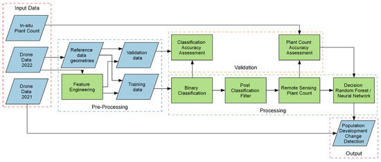
Figure 2.
Conceptual illustration of this study’s workflow—from input data to change detection map. Blue-colored parallelograms represent data, green-colored rectangles represent processing steps.
3.1. Model Training, Classification, and Validation
In this investigation, we applied two different approaches (RF and NN) to identify DM individuals. The RF classifier is an ensemble machine learning algorithm that combines the results of multiple decision trees to a single class assignment [45]. Each tree is constructed by drawing a random subset of the training data and features with replacement. RF does not require feature scaling (normalization or standardization) because it relies on decision trees that split data based on feature thresholds. We used the RF implementation of scikit-learn [46] and adopted the suggested set of hyperparameters by [47], which are summarized in Table 3. We did not perform additional hyperparameter tuning, as the literature suggests these settings to be a sensible default RF model parameterization in the context of RS data. Furthermore, the same setting for an RF model showed promising results in [36].
Table 3.
Random Forest parameters modified for this study. The other parameters are scikit-learn’s default values.
For RF, we adopted the selection of image features from [36], as they showed a considerable impact on the model’s ability to differentiate between the DM-positive and the DM-negative class. The feature selection consisted of the red, red-edge and near-infrared band of the sensor and four additional vegetation indices that we derived from the drone data. The vegetation indices are listed in Table 4.
Table 4.
Vegetation index selection to differentiate between the DM-positive and DM-negative class. Abbreviations: B = blue band; G = green band; R = red band; NIR = near-infrared band.
We employed a densely connected NN with double hidden layer. The network was trained using only the spectral bands. The same training–validation split as RF was utilized in the case of the NN. We employed the trained network for the predictions (presence or absence of DM) with the prediction data, which did not participate while training and validating the NN.
We validated the classification qualitatively and quantitatively. For the latter, we used the validation data with the F1 score, which is defined as
where precision is defined as the ratio of true positive class assignments and the sum of true positive and false positive class assignments. Recall is defined as the ratio of true positive class assignments and the sum of true positive and false negative class assignments.
For the qualitative accuracy assessment, we visually assessed the performance of each model for their ability to detect the DM-positive class and how well the model coped with the ambiguity problem and potential systematic misclassifications.
3.2. Monitoring the DM Population Development
Monitoring the population development of DM requires a reproducible and spatially explicit count of plant individuals. To achieve this, we employed the RSPC methodology, as described in [36], in two consecutive flowering seasons. In summary, we applied the following processing steps to the RF and NN classification results separately:
- 1.
- Polygonize neighboring DM-positive pixels into image objects.
- 2.
- Calculate a filter threshold based on the image object-level median value of the MaVI.
- 3.
- Assign the DM-negative class to all pixels within an image object below the object median filter threshold.
We then aggregated the remaining DM-positive pixels on a predefined reference grid, where one grid cell had a size of 1 m². The aggregation is based on the assumption that one DM-positive pixel corresponds to one DM individual.
To assess the accuracy of the RF- and NN-based RSPC, we compared each filtered result with the in situ data described in Section 2.4. We applied a squared buffer (1-m side length) to the GPS-logged point of each reference square. We then used the resulting polygon to sample pixels classified as DM-positive. The agreement between the RSPC results and the in situ data is illustrated in scatterplots and quantified using the R² metric. The deviation of the RSPC and the in situ plant count is quantified by the Root-Mean-Square-Error (RMSE) metric. Both metrics are described in the following equations:
where is the RSPC, is the in situ plant count, is the average plant count, and n is the number of reference squares. When applied to a single year, RSPC documents the distribution of a DM population in a comprehensive spatial manner. Multi-year RSPCs allow conservationists to monitor the population development of DM. In this study, we illustrate the population development using a change detection map. Since we used the same reference grid for both the years, we reported the net gain and loss of DM individuals per unit area. The change in a grid cell is defined as follows:
where is the change of DM individuals between two years. corresponds to the latest RSPC in 2022 and to RSPC of the year 2021.
4. Results and Discussion
4.1. Accuracy Assessment of Classification Methods
The predictive accuracy of both classifiers on the validation data is very high (see Table 5 and Table 6). We observed an F1-score of 0.99 for both RF and NN-based approach. The accuracy metrics indicated an apparent nearly perfect capability of both model types to differentiate between the DM-positive and the DM-negative class. For RF, the high F1-score confirmed the capability of the feature selection derived from [36] to identify magenta-colored vegetation. For NN, the high F1-score indicated that the classifier was able to learn important feature relationships from a simpler feature set (only the spectral bands).
Table 5.
The confusion matrix shows the predictive performance of the NN classifier on the validation dataset of the 2022 drone flight.
Table 6.
The confusion matrix shows the predictive performance of the RF classifier on the validation dataset of the 2022 drone flight.
However, it is important to note that the model accuracies might have been influenced by certain methodological limitations in this study’s reference data sampling process. The sampling process is non-probabilistic for the DM-positive class and only partially probabilistic for the DM-negative class [51,52]. Furthermore, the limited size of the validation data might have led to inflated accuracy scores. One potential strategy to address these limitations could have been to augment the validation dataset by sampling new reference points. For our study, however, this was unfeasible since the ambiguity problem limited our ability to confidently identify additional DM-positive points without introducing image artifacts to the reference data.
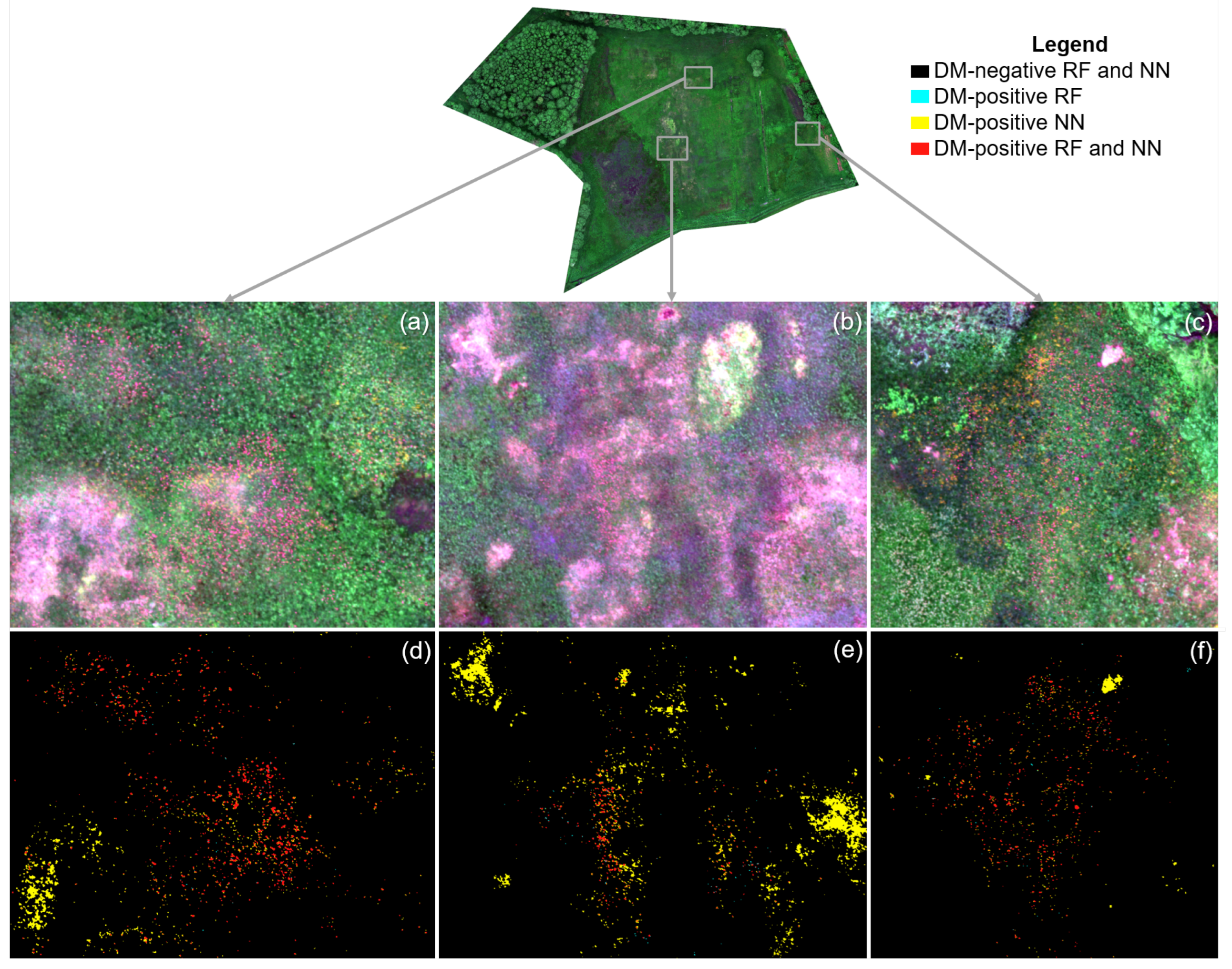
The qualitative accuracy assessment revealed noticeable quality differences between the RF and NN classification results, which are illustrated in Figure 3. The NN was able to identify slightly more true-positive DM pixels than the RF classifier. However, the share of false-positive DM-positive pixels was much higher using the NN. The majority of false-positive class assignments for both classifiers can be attributed to the ambiguity problem. The NN classifier was far less able to cope with the sensor artifacts (see Figure 3d,e). We attribute this limitation to the sensitivity of the NN to the specific architectures used to arrange the computational units [53]. Domain-specific insights have been observed to play a crucial role in the organization of the underlying computational units architecture, which consequently influences the final prediction performance of a NN. We noticed a rare but systematic failure of the RF classifier to distinguish magenta-colored vegetation and woody vegetation (tree branches), which might be explained by their similar spectral response [36], as we observed particularly in the blue, green, and red band. Depending on the influence of the ambiguity problem on a pixel, a partial overlap in the feature space in the red-edge and NIR bands may also exist, which further reduces class separability. The misconception was more severely present in the NN results. A possible explanation for the increased confusion might have been the simpler set of input features (i.e., the image bands) compared to the RF model. The NN additionally had a severe problem distinguishing magenta-colored vegetation and bare soil or shadow surfaces.
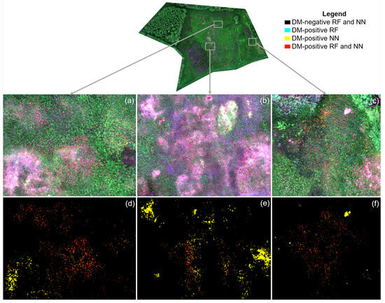
Figure 3.
Comparison of RF and NN classification result (2022). Subfigures (a–c) are contrast-enhanced RGB true color reference images of subfigures (d–f). Subfigures (d–f) illustrate the pixel-level agreement of the RF and NN classifiers, respectively.
The NN can be further optimized to extract a better performance by fine-tuning the hyperparameters (epochs, number of neurons, connection dropouts, etc.). In order to avoid information redundancy, we only used the spectral bands as training features. Considering the complexity of the NN (densely connected double layer) we used for this study, we assumed that the network was capable of self-learning the additional feature representations contributed by the vegetation indices. We ensured that the network was not over-trained to specifically fit the given data (for merely obtaining a higher performance) but rather considered the generalization of the predictions. Moreover, it is important to note that the success of NNs is not universal across all domains. This is particularly true for learning problems without any special structure or under somewhat limited data conditions. Under such circumstances, NNs do not perform better than traditional machine learning methods, such as RF [53]. Unlike the robust performance of RF, irrespective of the data domain, arising as a result of their randomized ensemble approach, NNs are highly prone to overfitting. The use of a generic layered architecture of the computation units may not achieve favorable outcomes. On the contrary, RFs have built-in mechanisms to combat overfitting. By constructing an ensemble of decision trees and aggregating their predictions, they tend to generalize well to unseen data without extensive hyperparameter tuning.
Unlike several Earth Observation investigations promising the ultimate performance with NNs, we observed and reported (with RF) a more realistic scenario reported by fundamental machine learning investigations [53]. However, it’s not universally true that RF outperforms NN or vice versa. RF might appear superior in some scenarios. It tends to perform well with relatively small- to medium-sized datasets. NNs are more sensitive to data quality. If the dataset is small or lacks diversity, NNs may be affected by noise and, consequently, struggle to generalize well. In general, RF can handle noisy data and is less sensitive to outliers. Due to their decision tree structure, RF provides better interpretability as compared to deep NNs, which are often treated as "black box" models and are difficult to train effectively under limited data conditions. On the contrary, NNs can outperform RF when non-linear feature relationships inherent to the classification problem are too complex to be captured by an RF model, provided a training dataset of sufficiently large size and high quality is available. From a computational perspective, NNs may also be preferred over RF when scalability becomes an issue. NNs can be accelerated and distributed across multiple graphics or tensor processing units, allowing them to scale efficiently to handle massive datasets and complex architectures. Training an RF model can also be parallelized to some extent but may not scale as effectively for certain tasks.
4.2. Drone-Based Plant Count Accuracy
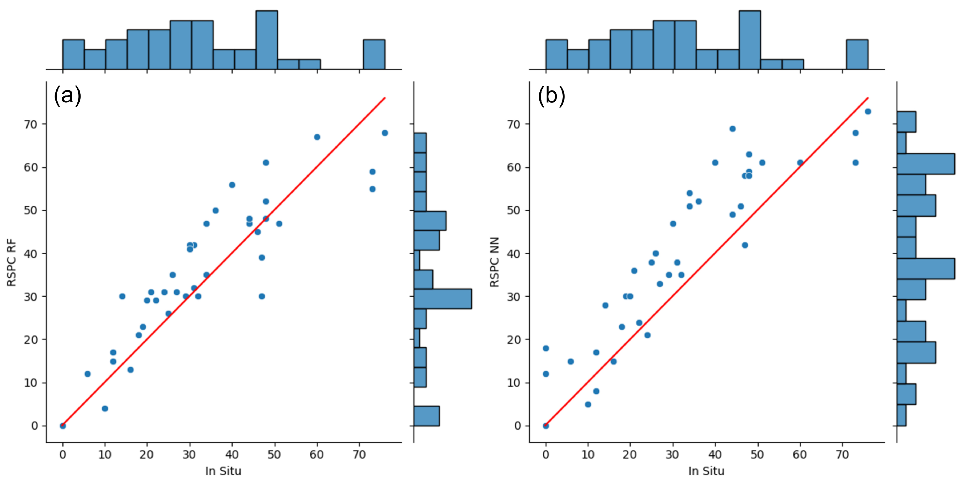
The RF-based RSPC showed good agreement with the in situ plant count. We observed an R² of 0.8 and a RMSE of 8.5 DM individuals/m² between the two methods. The NN-based RSPC showed reasonable agreement with the in situ data, with an R² of 0.63 and a RMSE of 11.4 DM individuals/m². Figure 4 illustrates that both RSPCs tended to overestimate the plant counts, with the NN-based RSPC showing a relatively pronounced overestimation. This phenomenon is associated with the characteristics of the NN classification results. The NN classifier confused woody vegetation, bare soil, and shadowed surfaces for the DM-positive class. The RSPC filter reduced these systematic misclassifications, but in the end, they persisted to a certain extent and inflated the NN-based RSPC. This was particularly evident in the reference squares where the in situ plant count was 0. In two of these squares, the majority of the area is covered by bare soil, which the NN classifiers confused for the DM-positive class.
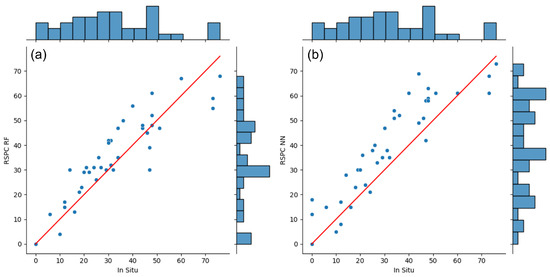
Figure 4.
Comparison of RSPC in the RF (a) and NN (b) results in the in situ data. The scatterplots show the agreement between RSPC and in situ plant counts. The red lines show theoretical lines of perfect agreement for orientation. The histograms show the frequency distribution of each plant count method individually.
Underestimation rarely occurred in both RSPCs but was slightly more noticeable in the RF-based RSPC. Both RSPCs considerably underestimated the reference squares associated with very high in situ plant counts (>70 DM individuals/m²), which may be the result of the RSPC filter. A high number of DM individuals in one reference square will most likely lead to few large DM image objects. In large DM image objects, the RSPC filter drops DM-positive pixels more greedily as compared to smaller DM image objects and, therefore, tends to lose some valid DM positive pixels. The increased pixel size in 2022 addressed the issue of image artifacts by enhancing the SNR [54], which consequently played a role in improving the detection performance of DMs. The performance increased from a RMSE of 12 DM individuals/m² [36] to 8.5 DM individuals/m². The RSPC accuracy assessment may be subject to uncertainties related to the spatial inaccuracies of the GPS devices used to locate the reference squares. We paid special attention to maximize the logging precision and reliability via cross validation of multiple logging methods and devices. However, we have no quantified measurement available on the performance improvement relative to the device precision reported by the manufacturer when operated in normal GPS mode.
4.3. DM Population Development in the Lehmkuhlen Reservoir
The classification and RSPC accuracy assessment indicated that the RF-based approach performed better than the NN-based approach. We, therefore, decided to assess the population development using only the RF-based results.
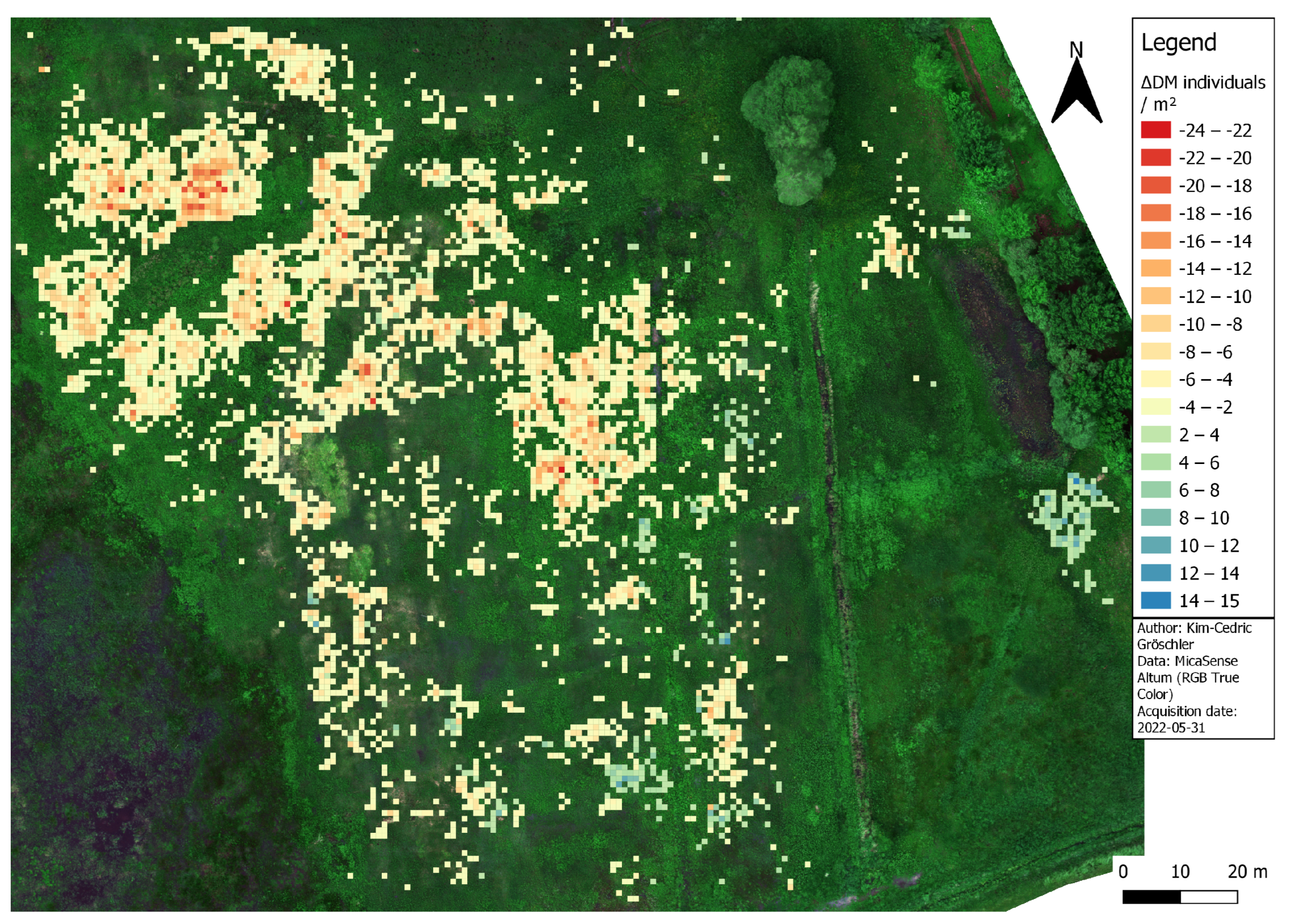
In 2022, our analysis indicated an overall decrease in DM individuals compared to the survey conducted in 2021 (see Figure 5). On average, we calculated a loss of 62% of DM individuals per unit area, with a maximum loss for a single grid cell of 24 DM individuals. The loss covered most of the area and was especially distinct in the northern part of the study site, which we identified as a DM hotspot in [36]. For this area, we were hardly able to report any grid cells with an increasing DM count. In the southern part of the study site, there were also fewer DM individuals; however, the decrease was less pronounced. Additionally, we reported multiple smaller spots with a net gain of DM individuals, with a maximum gain of 15 DM individuals for a single grid cell. In the eastern part, just south of the small pond, we identified a notable increase, which corroborates with a seed material transfer conducted by conservationists. To expand the DM habitat, they transferred grass and DM cuttings from the hotspot area to this part of the reservoir, as it showed favorable growing conditions but lacked DM individuals for natural seed transfer. Our results confirmed that the seed material transfer was successful in 2022 and that the DM habitat could be expanded eastward.
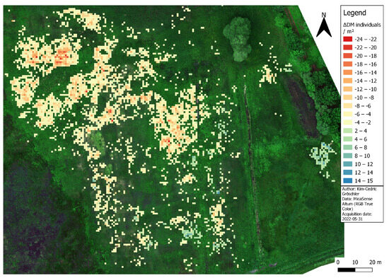
Figure 5.
Population development of Dactylorhiza majalis in the Lehmkuhlen reservoir. The map shows the net change of plants per unit area as detected during the flowering seasons of 2021 and 2022, respectively.
The overall loss of DM individuals in 2022 could be explained by natural fluctuations in the DM population. However, the change detection might also have some inherent uncertainties. The loss might be amplified in grid cells containing a substantial number of DM individuals in 2021 due to the increased severity of the ambiguity problem during that year. Therefore, the count of DM-positive pixels in 2021 was higher than the number of DM-positive pixels in 2022. Since we applied the RSPC filter separately to the two datasets, its influence on the plant counts might differ, which in turn might influence the change detection. We expect this factor to have a greater influence on the plant loss than on the gain. Another source of uncertainty arose from the different spatial resolution of both drone datasets. The 2022 dataset had a slightly larger pixel size at 4 cm, as opposed to the 3.4 cm pixel size in the 2021 dataset. Therefore, the number of available pixels per grid cell was lower in 2022. Consequently, this might have led to a slightly decreased count of DM individuals in 2022 relative to 2021. However, we argue that this factor might have had a negligible impact on grid cells of low to medium RSPC results. For high RSPC grid cells, this might have led to a minor loss overestimation or a minor gain underestimation. Undetected DM individuals in one of the years might have also influenced the DM change calculation. But we expect this factor to be less important since the RF-based detection worked quite reliably.
4.4. Implications for Practical Nature Conservation
In this study, we presented an RS-based alternative to monitor the DM population development and visualizations that communicate effectively to a conservationist audience. The approach supplements conventional plant survey methods in a spatio-temporal manner, which is rarely available due to the limited monetary and personnel resources in the field of nature conservation. Furthermore, it has the potential to reduce the reliance of plant count surveys on the workforce of (non-expert) volunteers. Our approach is not only reproducible but also easily scalable, enabling the consistent and objective monitoring of DM populations over time. It allows conservationists to identify areas with a declining DM population and implement targeted interventions to sustain the species. Additionally, the success of conservation measures can be visualized and documented. Since our approach exploits the spectral response corresponding to the flower color, conservationists expressed its possible applicability to monitor the population development of other plant species, such as Dactylorhiza incarnata or Lythrum salicaria.
Drone-based data acquisition provides additional benefits for practical nature conservation. Traditional ground-based surveys are time-consuming and labor-intensive, while drones allow coverage of larger territories efficiently, reducing fieldwork time and costs. Limited monetary resources can, therefore, be allocated more effectively, e.g., to ensure a longer duration of a monitoring program. The proposed method also prevents plant damage due to trampling, as the drone pilot’s need to access the area of interest is generally limited to the margins of the study site to manage calibration targets. This poses a minimal disturbance to the habitat compared to traditional field campaigns.
5. Conclusions
In summary, we showed the capabilities of an RS-based approach to monitor the population development of DM within a high nature value grassland site. Leveraging very high-spatial-resolution drone imagery, we observed the net change of DM individuals over two consecutive flowering seasons using a spatially consistent reference grid.
Our study revealed an overall decrease in the DM population in the Lehmkuhlen reservoir during 2022 compared to the baseline conditions of 2021. The results indicated that only a limited number of grid cells exhibited an increase in DM individuals. The magnitude of this gain was typically less pronounced as compared to the magnitude of the observed losses. We validated the positive outcome of a DM seed transfer event conducted by the conservationists. Our results provide spatio-temporal information for conservationists that could either be only attainable with significant resources or lack the comprehensive spatial scale. Monitoring over two consecutive flowering seasons highlighted the positive outcomes of targeted conservation measures. Future research programs will benefit from the proposed methodology for long-term monitoring and reveal the temporal development trend of the indicator species. The proposed methodology can be modified and extended to other indicator plant species as well as geographical locations.
We tested the ability of two classifiers (RF and NN) with different levels of complexity to provide a data basis for the RSPC. The results showed that the RF-based RSPC produced better results than the NN-based RSPC (R² of 0.8 vs 0.63, respectively, in comparison to in situ data). We identified systematic misclassifications of bare soil and shadow surfaces with magenta-colored vegetation as the main limiting factor for NN. With a RMSE of 8.5 DM individuals/m², the performance of the RF-based RSPC was comparable to traditional plant-mapping approaches.
Our study underlines the efficacy of employing drone data and machine learning techniques for ecological assessments. By unveiling the nuances in the DM population trends and migration successes, we demonstrate that drone-based surveys can indeed supplement conservation efforts and reduce data scarcity.
Author Contributions
Conceptualization, K.-C.G. and N.O.; methodology, K.-C.G., A.M. and S.K.R.; software, K.-C.G. and A.M.; validation, K.-C.G. and A.M.; formal analysis, K.-C.G.; investigation, K.-C.G.; resources, N.O.; data curation, K.-C.G.; writing—original draft preparation, K.-C.G. and A.M.; writing—review and editing, N.O.; visualization, K.-C.G.; supervision, N.O.; project administration, N.O.; funding acquisition, N.O. All authors have read and agreed to the published version of the manuscript.
Funding
This study was funded by the German Federal Environmental Foundation (Deutsche Bundesstiftung Umwelt DBU) under grant number 35544/01 within the project VeGEMite.
Data Availability Statement
The data presented in this study are available on reasonable request from the corresponding author. The data are not publicly available due to copyright restrictions.
Acknowledgments
We gratefully acknowledge the considerable effort of Jessica Krause in conducting the field mapping. The authors also thank the anonymous reviewers for their valuable comments and suggestions to improve the quality of the paper.
Conflicts of Interest
The authors declare no conflict of interest.
References
- Hobohm, C.; Bruchmann, I. Endemische Gefäßpflanzen und ihre Habitate in Europa – Plädoyer für den Schutz der Grasland-Ökosysteme; Technical Report 21; Berichte der Reinhold-Tüxen-Gesellschaft: Geestland, Germany, 2009. [Google Scholar]
- Kuhn, T.; Domokos, P.; Kiss, R.; Ruprecht, E. Grassland Management and Land Use History Shape Species Composition and Diversity in Transylvanian Semi-Natural Grasslands. Appl. Veg. Sci. 2021, 24, e12585. [Google Scholar] [CrossRef]
- Öckinger, E.; Smith, H.G. Landscape Composition and Habitat Area Affects Butterfly Species Richness in Semi-Natural Grasslands. Oecologia 2006, 149, 526–534. [Google Scholar] [CrossRef]
- Loos, J.; Gallersdörfer, J.; Hartel, T.; Dolek, M.; Sutcliffe, L. Limited Effectiveness of EU Policies to Conserve an Endangered Species in High Nature Value Farmland in Romania. Ecol. Soc. 2021, 26. [Google Scholar] [CrossRef]
- Bakker, J.P.; Berendse, F. Constraints in the Restoration of Ecological Diversity in Grassland and Heathland Communities. Trends Ecol. Evol. 1999, 14, 63–68. [Google Scholar] [CrossRef] [PubMed]
- Habel, J.C.; Dengler, J.; Janišová, M.; Török, P.; Wellstein, C.; Wiezik, M. European Grassland Ecosystems: Threatened Hotspots of Biodiversity. Biodivers. Conserv. 2013, 22, 2131–2138. [Google Scholar] [CrossRef]
- Hopkins, A.; Del Prado, A. Implications of Climate Change for Grassland in Europe: Impacts, Adaptations and Mitigation Options: A Review. Grass Forage Sci. 2007, 62, 118–126. [Google Scholar] [CrossRef]
- Van Oijen, M.; Bellocchi, G.; Höglind, M. Effects of Climate Change on Grassland Biodiversity and Productivity: The Need for a Diversity of Models. Agronomy 2018, 8, 14. [Google Scholar] [CrossRef]
- European Union. Council Directive 92/43/EEC of 21 May 1992 on the Conservation of Natural Habitats and of Wild Fauna and Flora; European Union: Brussels, Belgium, 1992.
- European Union. Directive 2009/147/EC of the European Parliament and of the Council of 30 November 2009 on the Conservation of Wild Birds (Codified Version); European Union: Brussels, Belgium, 2009.
- Török, P.; Brudvig, L.A.; Kollmann, J.; Price, J.N.; Tóthmérész, B. The Present and Future of Grassland Restoration. Restor. Ecol. 2021, 29, e13378. [Google Scholar] [CrossRef]
- Carignan, V.; Villard, M.A. Selecting Indicator Species to Monitor Ecological Integrity: A Review. Environ. Monit. Assess. 2002, 78, 45–61. [Google Scholar] [CrossRef]
- Swarts, N.D.; Dixon, K.W. Terrestrial Orchid Conservation in the Age of Extinction. Ann. Bot. 2009, 104, 543–556. [Google Scholar] [CrossRef]
- Phillips, R.D.; Reiter, N.; Peakall, R. Orchid Conservation: From Theory to Practice. Ann. Bot. 2020, 126, 345–362. [Google Scholar] [CrossRef] [PubMed]
- Janečková, P.; Wotavová, K.; Schödelbauerová, I.; Jersáková, J.; Kindlmann, P. Relative Effects of Management and Environmental Conditions on Performance and Survival of Populations of a Terrestrial Orchid, Dactylorhiza Majalis. Biol. Conserv. 2006, 129, 40–49. [Google Scholar] [CrossRef]
- Dullau, S.; Richter, F.; Adert, N.; Meyer, M.; Hensen, H.; Tischew, S. Handlungsempfehlung Zur Populationsstärkung und Wiederansiedlung von Dactylorhiza Majalis Am Beispiel Des Biosphärenreservates Karstlandschaft Südharz; Technical report; Hochschule Anhalt: Bernburg, Germany, 2019. [Google Scholar]
- Lohr, M.; Margenburg, B.; Margenburg, B. Das Breitblättrige Knabenkraut Dactylorhiza majalis–Orchidee des Jahres 2020. J. Eur. Orch. 2020, 52, 287–323. [Google Scholar]
- Metzing, D.; Garve, E.; Matzke-Hajek, G.; Adler, J.; Bleeker, W.; Breunig, T.; Caspari, S.; Dunkel, F.G.; Fritsch, R.; Gottschlich, G.; et al. Rote Liste Und Gesamtartenliste Der Farn-Und Blütenpflanzen (Trachaeophyta) Deutschlands. Naturschutz Biol. Vielfalt 2018, 70, 13–358. [Google Scholar]
- Wotavová, K.; Balounová, Z.; Kindlmann, P. Factors Affecting Persistence of Terrestrial Orchids in Wet Meadows and Implications for Their Conservation in a Changing Agricultural Landscape. Biol. Conserv. 2004, 118, 271–279. [Google Scholar] [CrossRef]
- Reinhard, H.R.; Gölz, P.; Peter, R.; Wildermuth, H. Die Orchideen Der Schweiz und Angrenzender Gebiete; Fotorotar AG: Zürich, Switzerland, 1991. [Google Scholar] [CrossRef]
- Gregor, T.; Saurwein, h.P. Wer erhält das Großblättrige Knabenkraut (Dactylorhiza majalis); Technical Report; Beiträge zur Naturkunde in Osthessen: Neuhof, Germany, 2010. [Google Scholar]
- Messlinger, U.; Pape, T.; Wolf, S. Erhaltungsstrategien für das Breitblättrige Knabenkraut (Dactylorhiza majalis) in Stadt und Landkreis Ansbach; Technical Report; RegnitzFlora-Mitteilungen des Vereins zur Erforschung der Flora des Regnitzgebietes: Nürnberg, Germany, 2018. [Google Scholar]
- Pescott, O.L.; Walker, K.J.; Harris, F.; New, H.; Cheffings, C.M.; Newton, N.; Jitlal, M.; Redhead, J.; Smart, S.M.; Roy, D.B. The Design, Launch and Assessment of a New Volunteer-Based Plant Monitoring Scheme for the United Kingdom. PLoS ONE 2019, 14, e0215891. [Google Scholar] [CrossRef]
- Hunter, A.; Rollins, R. Motivational Factors of Environmental Conservation Volunteers. In Proceedings of the Sixth International Conference of Science and the Management of Protected Areas, Ecosystem Based Management: Beyond Boundaries, Wolfville, NS, Canada, 21–26 May 2010; Acadia University: Wolfville, NS, Canada, 2010. [Google Scholar]
- Albergoni, A.; Bride, I.; Scialfa, C.T.; Jocque, M.; Green, S. How Useful Are Volunteers for Visual Biodiversity Surveys? An Evaluation of Skill Level and Group Size during a Conservation Expedition. Biodivers. Conserv. 2016, 25, 133–149. [Google Scholar] [CrossRef]
- McKinley, D.C.; Miller-Rushing, A.J.; Ballard, H.L.; Bonney, R.; Brown, H.; Cook-Patton, S.C.; Evans, D.M.; French, R.A.; Parrish, J.K.; Phillips, T.B.; et al. Citizen Science Can Improve Conservation Science, Natural Resource Management, and Environmental Protection. Biol. Conserv. 2017, 208, 15–28. [Google Scholar] [CrossRef]
- Conrad, C.C.; Hilchey, K.G. A Review of Citizen Science and Community-Based Environmental Monitoring: Issues and Opportunities. Environ. Monit. Assess. 2011, 176, 273–291. [Google Scholar] [CrossRef]
- Pettorelli, N.; Safi, K.; Turner, W. Satellite Remote Sensing, Biodiversity Research and Conservation of the Future. Philos. Trans. R. Soc. B Biol. Sci. 2014, 369, 20130190. [Google Scholar] [CrossRef]
- Horton, R.; Cano, E.; Bulanon, D.; Fallahi, E. Peach Flower Monitoring Using Aerial Multispectral Imaging. J. Imaging 2017, 3, 2. [Google Scholar] [CrossRef]
- Fang, S.; Tang, W.; Peng, Y.; Gong, Y.; Dai, C.; Chai, R.; Liu, K. Remote Estimation of Vegetation Fraction and Flower Fraction in Oilseed Rape with Unmanned Aerial Vehicle Data. Remote Sens. 2016, 8, 416. [Google Scholar] [CrossRef]
- Abdel-Rahman, E.; Makori, D.; Landmann, T.; Piiroinen, R.; Gasim, S.; Pellikka, P.; Raina, S. The Utility of AISA Eagle Hyperspectral Data and Random Forest Classifier for Flower Mapping. Remote Sens. 2015, 7, 13298–13318. [Google Scholar] [CrossRef]
- Sulik, J.J.; Long, D.S. Spectral Indices for Yellow Canola Flowers. Int. J. Remote Sens. 2015, 36, 2751–2765. [Google Scholar] [CrossRef]
- Landmann, T.; Piiroinen, R.; Makori, D.M.; Abdel-Rahman, E.M.; Makau, S.; Pellikka, P.; Raina, S.K. Application of Hyperspectral Remote Sensing for Flower Mapping in African Savannas. Remote Sens. Environ. 2015, 166, 50–60. [Google Scholar] [CrossRef]
- Carl, C.; Landgraf, D.; van der Maaten-Theunissen, M.; Biber, P.; Pretzsch, H. Robinia Pseudoacacia L. Flower Analyzed by Using An Unmanned Aerial Vehicle (UAV). Remote Sens. 2017, 9, 1091. [Google Scholar] [CrossRef]
- Severtson, D.; Callow, N.; Flower, K.; Neuhaus, A.; Olejnik, M.; Nansen, C. Unmanned Aerial Vehicle Canopy Reflectance Data Detects Potassium Deficiency and Green Peach Aphid Susceptibility in Canola. Precis. Agric. 2016, 17, 659–677. [Google Scholar] [CrossRef]
- Gröschler, K.C.; Oppelt, N. Using Drones to Monitor Broad-Leaved Orchids (Dactylorhiza Majalis) in High-Nature-Value Grassland. Drones 2022, 6, 174. [Google Scholar] [CrossRef]
- Shen, M.; Chen, J.; Zhu, X.; Tang, Y. Yellow Flowers Can Decrease NDVI and EVI Values: Evidence from a Field Experiment in an Alpine Meadow. Can. J. Remote Sens. 2009, 35, 8. [Google Scholar] [CrossRef]
- Shen, M.; Chen, J.; Zhu, X.; Tang, Y.; Chen, X. Do Flowers Affect Biomass Estimate Accuracy from NDVI and EVI? Int. J. Remote Sens. 2010, 31, 2139–2149. [Google Scholar] [CrossRef]
- Nowak, M.M.; Dziob, K.; Bogawski, P. Unmanned Aerial Vehicles (UAVs) in Environmental Biology: A Review. Eur. J. Ecol. 2018, 4, 56–74. [Google Scholar] [CrossRef]
- Oh, S.; Chang, A.; Ashapure, A.; Jung, J.; Dube, N.; Maeda, M.; Gonzalez, D.; Landivar, J. Plant Counting of Cotton from UAS Imagery Using Deep Learning-Based Object Detection Framework. Remote Sens. 2020, 12, 2981. [Google Scholar] [CrossRef]
- Valente, J.; Sari, B.; Kooistra, L.; Kramer, H.; Mücher, S. Automated Crop Plant Counting from Very High-Resolution Aerial Imagery. Precis. Agric. 2020, 21, 1366–1384. [Google Scholar] [CrossRef]
- Seer, F.K.; Schrautzer, J. Status, Future Prospects, and Management Recommendations for Alkaline Fens in an Agricultural Landscape: A Comprehensive Survey. J. Nat. Conserv. 2014, 22, 358–368. [Google Scholar] [CrossRef]
- Schrautzer, J.; Trepel, M. Niedermoore im Östlichen Hügelland. TUEXENIA 2014, 7, 47–49. [Google Scholar]
- MicaSense. MicaSense Altum™ and DLS 2 Integration Guide; MicaSense: Seattle, WA, USA, 2020. [Google Scholar]
- Breiman, L. Random Forests. Mach. Learn. 2001, 45, 5–32. [Google Scholar] [CrossRef]
- Pedregosa, F.; Varoquaux, G.; Gramfort, A.; Michel, V.; Thirion, B.; Grisel, O.; Blondel, M.; Müller, A.; Nothman, J.; Louppe, G.; et al. Scikit-Learn: Machine Learning in Python. arXiv 2012, arXiv:1201.0490. [Google Scholar] [CrossRef]
- Belgiu, M.; Drăguţ, L. Random Forest in Remote Sensing: A Review of Applications and Future Directions. ISPRS J. Photogramm. Remote Sens. 2016, 114, 24–31. [Google Scholar] [CrossRef]
- Vincini, M.; Frazzi, E.; D’Alessio, P. A Broad-Band Leaf Chlorophyll Vegetation Index at the Canopy Scale. Precis. Agric. 2008, 9, 303–319. [Google Scholar] [CrossRef]
- Gitelson, A.A.; Kaufman, Y.J.; Merzlyak, M.N. Use of a Green Channel in Remote Sensing of Global Vegetation from EOS-MODIS. Remote Sens. Environ. 1996, 58, 289–298. [Google Scholar] [CrossRef]
- Baret, F.; Guyot, G. Potentials and Limits of Vegetation Indices for LAI and APAR Assessment. Remote Sens. Environ. 1991, 35, 161–173. [Google Scholar] [CrossRef]
- Stehman, S.V. Sampling Designs for Accuracy Assessment of Land Cover. Int. J. Remote Sens. 2009, 30, 5243–5272. [Google Scholar] [CrossRef]
- Waldner, F. The T Index: Measuring the Reliability of Accuracy Estimates Obtained from Non-Probability Samples. Remote Sens. 2020, 12, 2483. [Google Scholar] [CrossRef]
- Wang, S.; Aggarwal, C.; Liu, H. Using a Random Forest to Inspire a Neural Network and Improving on It. In Proceedings of the 2017 SIAM International Conference on Data Mining, Philadelphia, PA, USA, 27–29 April 2017. [Google Scholar] [CrossRef]
- Chen, T.; Catrysse, P.B.; El Gamal, A.; Wandell, B.A. How Small Should Pixel Size Be? In Proceedings of the Electronic Imaging, San Jose, CA, USA, 15 May 2000; Blouke, M.M., Sampat, N., Williams, G.M., Jr., Yeh, T., Eds.; SPIE: Washington, DC, USA, 2000; p. 451. [Google Scholar] [CrossRef]

Disclaimer/Publisher’s Note: The statements, opinions and data contained in all publications are solely those of the individual author(s) and contributor(s) and not of MDPI and/or the editor(s). MDPI and/or the editor(s) disclaim responsibility for any injury to people or property resulting from any ideas, methods, instructions or products referred to in the content. |
© 2023 by the authors. Licensee MDPI, Basel, Switzerland. This article is an open access article distributed under the terms and conditions of the Creative Commons Attribution (CC BY) license (https://creativecommons.org/licenses/by/4.0/).