In this section, we provide a detailed discussion of the design and development of CARLA+. In what follows next, we first discuss the PGM for modeling the environment followed by a thorough discussion on the design and development of CARLA+ which integrates a PGM framework with CARLA.
4.1. PGM for Modeling Complex Urban Environment
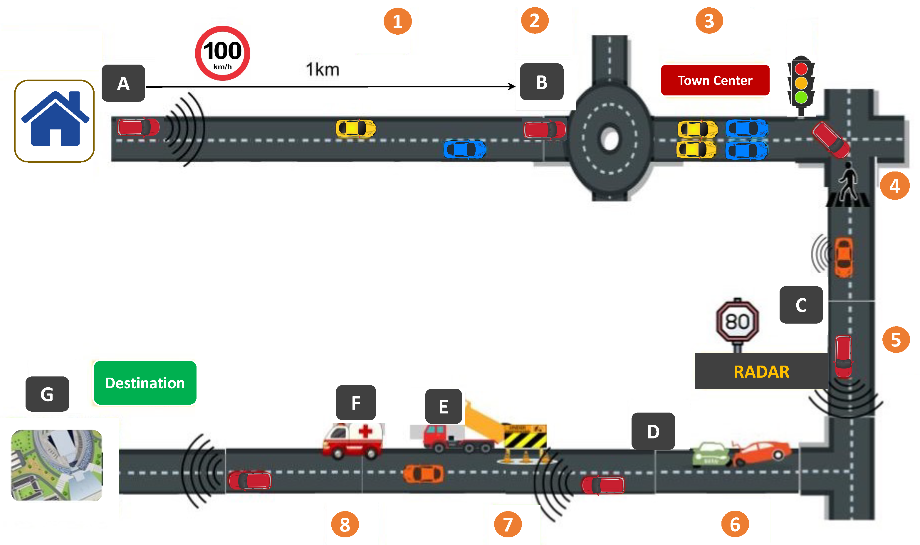
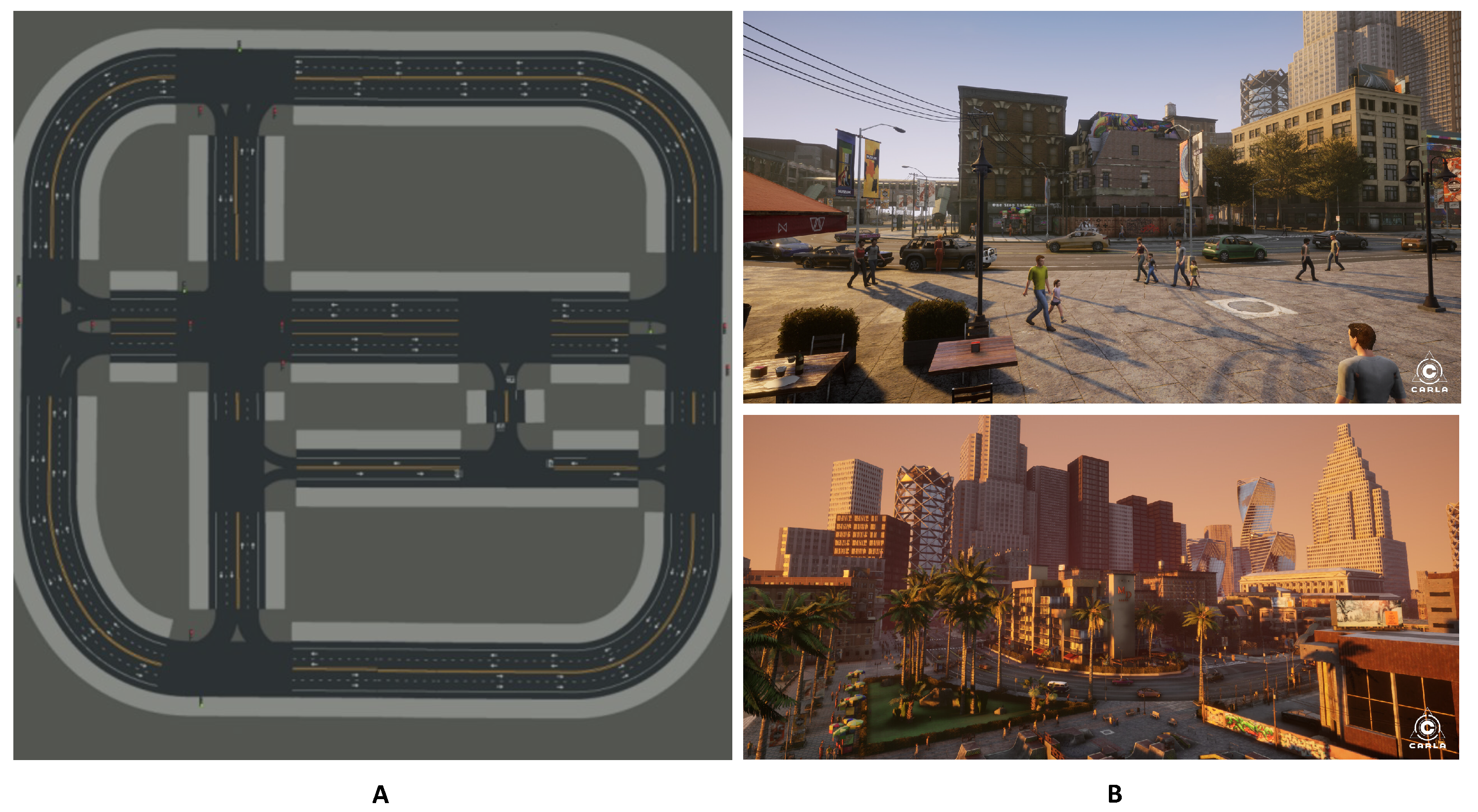
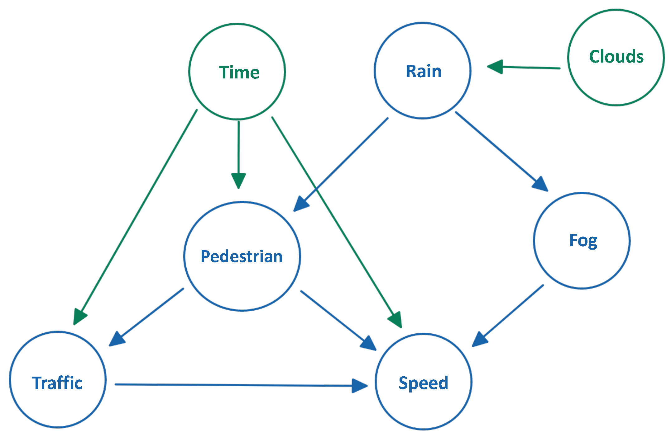
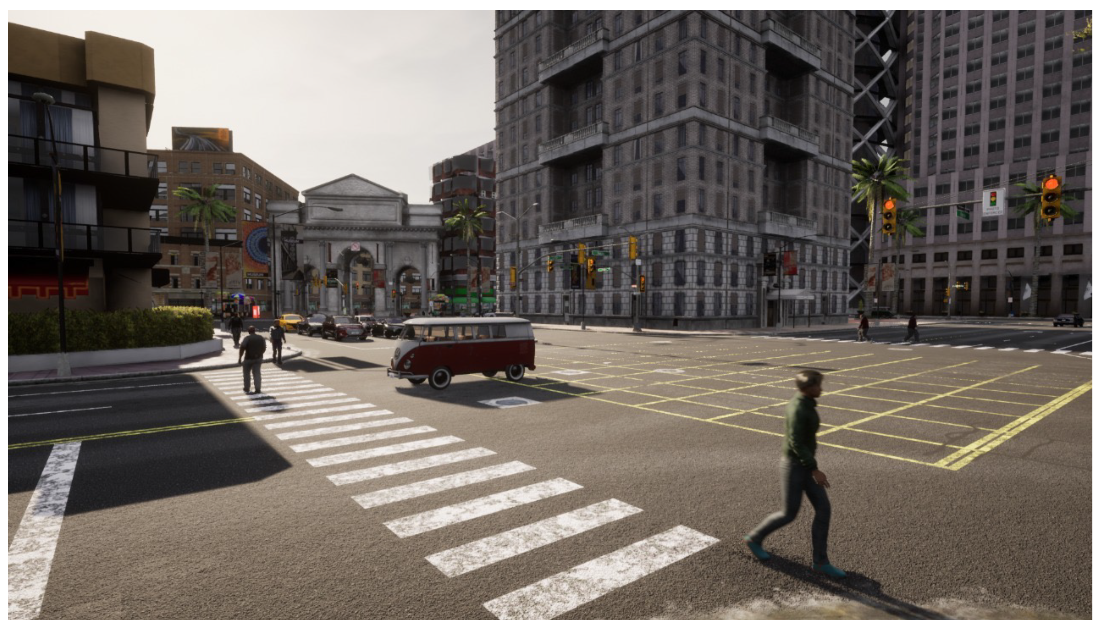
To capture the realistic dynamics of the complex urban environment such as the number of vehicles, the dynamic speed of the vehicles, the probability of pedestrians in an urban environment, the dynamic weather of the environment, and the time of the day, the probabilistic graphical model (PGM) is used. We aim at capturing the dynamically changing state of the environment, the partially observable state of the environment, and unprecedented events in the environment. To further understand the environment, consider
Figure 1 which explains some scenario scenes of the complex urban environment.
In what follows next, we discuss the motivation to opt for the PGM, which comes from the following facts:
It is instrumental in understanding the complex relationship between a set of random variables. This is an important feature because the considered problem domain involves several variables (e.g., number of vehicles, number of pedestrians, vehicle speed, weather state, time of the day, distance from other vehicles and objects, road markings, road signs, road traffic lights, etc.) Furthermore, these variables have an impact on one another, resulting in much more complex interparameter relationships;
It allows to reuse the knowledge accumulated over the different scenes and settings;
It allows for solving tasks such as inference learning. This feature is relevant to the considered collaborative autonomous driving problem domain since we are interested in estimating the probability distributions and probability functions in different use cases. For instance, when the probability is associated with the elements of action space in a specific use case, we are interested in achieving the optimal values of the associated probability values;
It allows the independence properties to represent high-dimensional data more compactly. The independence properties help in the considered problem domain by assisting in understanding the characteristics of a particular attribute separately from the rest of the system;
The concept of conditional independence brings in significant savings in terms of how to compute and represent the network structure.
A PGM models a joint probability distribution over a set of random variables . It is represented as a pair , which consists of a graph structure that codifies the dependent relationships between the random variables and a set of parameters . There are different types of PGM models, however, in this research, we implement the PGM model based on directed acyclic graphs (DAG). Given a PGM with a DAG , where X is a non-empty finite set of nodes and R is a set of edges, and three distinct subsets of variables of , is conditionally independent of given if d-separates and in .
We suppose that the set of variables
is arranged in accordance with a DAG
ancestral ordering, the parent nodes of
variable d-separates
from any prior variable in the ancestral ordering,
. This is to say that
is conditionally independent of any
given its parents,
. Based on this property, we express the joint probability distribution of
given the chain rule as:
when codified by a DAG-based PGM, it is factorized as:
Bayesian network (BN) models are DAG-based PGMs with all the discrete random variables, comprised of a DAG
and a set of parameters
. By taking DAGs into account, the joint probability distribution
can be factored using Equation (
2), which typically uses a much smaller set of
than the general factorization (Equation (
1)). The set of parameters
represents all the probability distributions,
. Each parameter
defines the probability that variable
takes its
possible value given that the parents
of
take their
value. Each variable
has a set of
values. As a result, the set of potential values for a random vector is the product of the sets of possible values for each
X such that the parent
of variable
takes
different values.
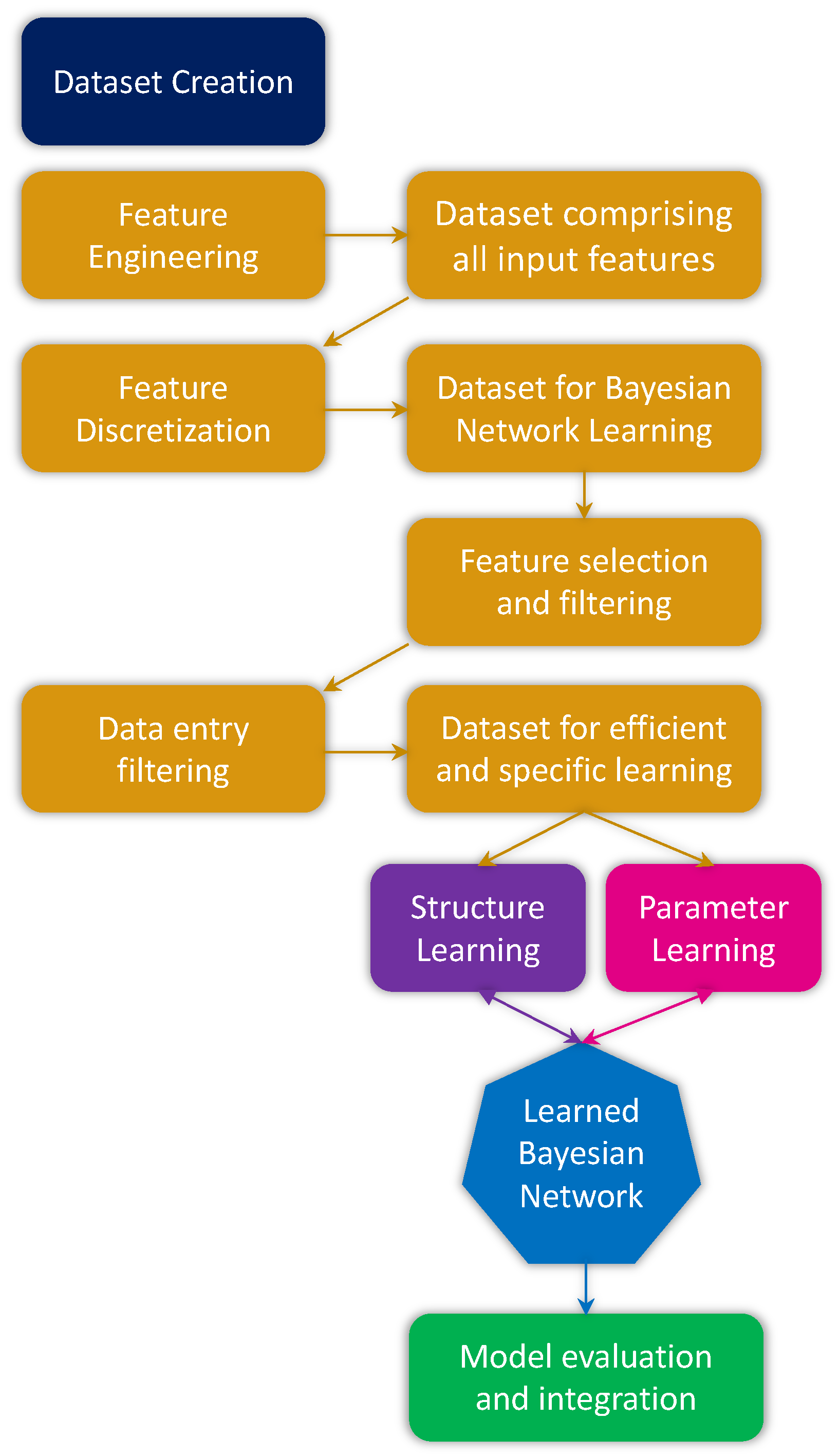
As the size of the model increases, the BN model derived from a set of examples becomes impractical. Therefore, we learn the BN. Generally, the process of learning a BN with DAG
and parameters
from a data set
comprising
n observations can be accomplished in two steps, Equation (
3). Following the
provision, the BN is learned in two stages: structural learning and parametric learning.
Finding the
that encodes the dependent structure of the data constitutes structure learning. In this research, we opt for the Hill Climbing (HC) search algorithm to learn the structure of the BN. In Algorithm 1, the initialization phases (steps 1 and 2) are followed by an HC search (step 3). HC executes local moves such as arc additions, deletions, and reversals to explore the area around the current candidate
in the space of all possible DAGs aiming to locate the
(if any) that raises the score Score
the most over
. Then, in each iteration, the HC attempts to add each potential arc that is not already present in
, as well as to delete and reverse each arc in the current optimal
. For all the remaining acyclic DAGs
, the HC calculates
=
. The new candidate
is the
with the highest
. If this DAG has
, then
becomes the new
, and
is set to
and HC moves to the next iteration. On the other hand, if
, the HC reaches an optimum.
| Algorithm 1. Hill-climbing search algorithm for structure learning |
Input: a dataset from X, an empty DAG , a score function Score . Output: the that maximizes the Score . - 1:
Compute the score of , = - 2:
Set and - 3:
Hill Climbing: repeat as long as increases. (a) For each potential arc addition, deletion, or reversal in resulting in a DAG: (i) Compute the score of updated , = (ii) and , then set and (b) If , set and
|
As a local search algorithm, the HC can get stuck in the local optima. Therefore, there are two simple approaches that are efficient to escape from the local optima:
Tabu List: it first moves away from by allowing up to additional local moves. These moves would generate DAGs with , therefore, the new candidate DAGs would have the highest even though if . Moreover, DAGs accepted as candidates in the last iterations would be saved in a list referred to as the tabu list. It will allow the algorithm to not revisit the recently seen structures aiming to guide the search towards unexplored regions of the space of the DAGs and this approach is referred to as Tabu search.
Random Restarts: multiple restarts up to r times would allow the algorithm to find the global optimum when at a local optimum.
Estimating the
based on the
produced by structure learning is what parameter learning entails. We employ the Bayesian Parameter Estimation to learn the parameters. When learning with a Bayesian approach, the Dirichlet distribution is used as an a priori distribution over all possible sets of parameters, and the maximum a posteriori probability (MAP) estimation—the set of parameters
with the highest a posteriori probability given the
and a graph structure
—is used to estimate the parameters.
Given a set of hyper-parameters
, which are the parameters of the a priori Dirichlet distribution that characterizes the prior knowledge about the
, we compute the set of
that maximizes this expression by using the formula below:
where in Equation (
5), the
is the total number of occurrences in
where the variable
is given its
value and the configuration of
is given its
instance,
and
.
4.2. Designing CARLA+
This section presents a detailed discussion on designing the CARLA+ comprises various crucial components. In what follows next, we discuss each component in detail.
4.2.1. CARLA Architecture
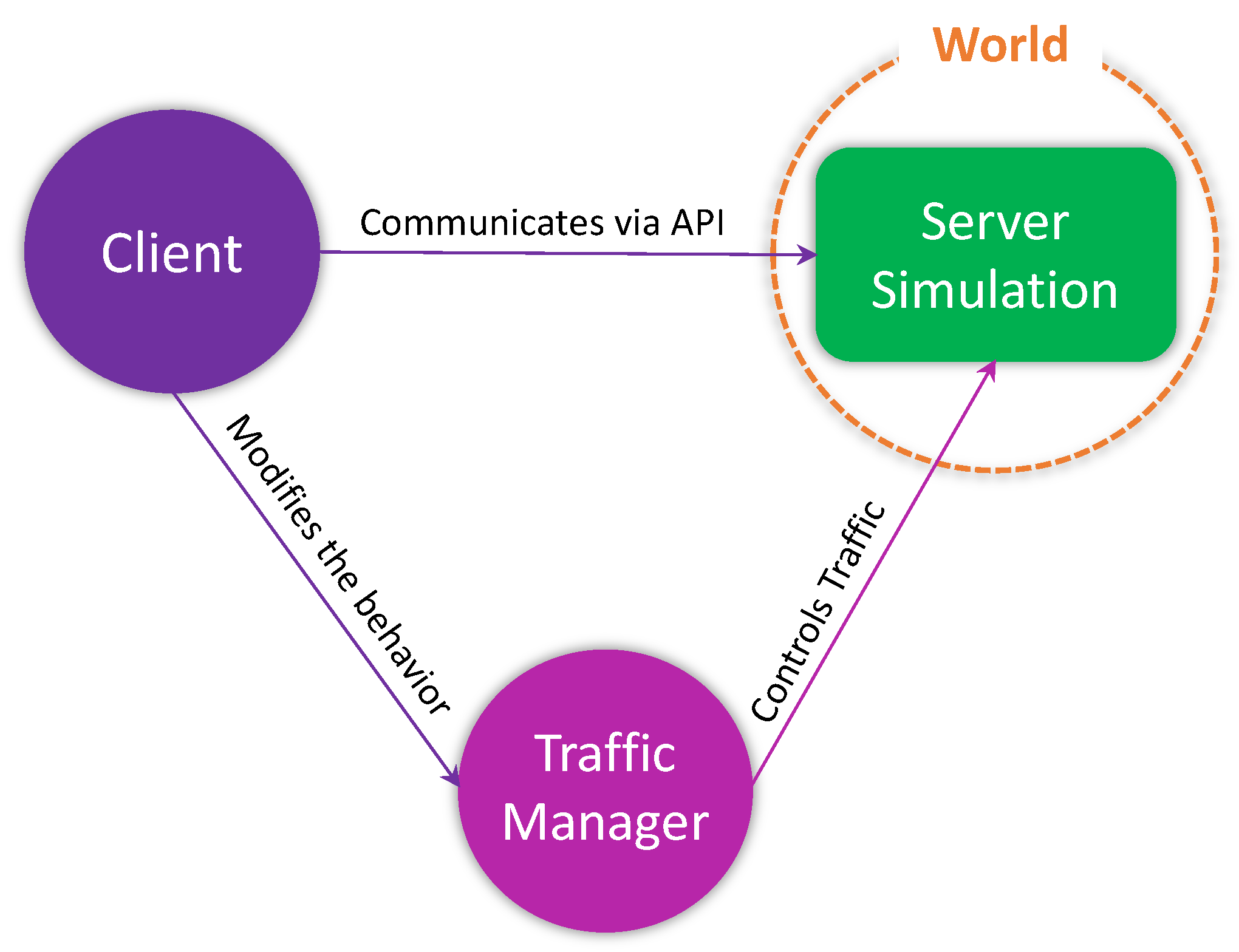
CARLA utilizes the client-server model for its operation where the server runs the actual simulation and the client is responsible to communicate and controlling that simulation. The CARLA client communicates with the CARLA server using the provided API. Therefore, to use the CARLA client, we first establish a connection with the CARLA server running on a specific IP and port. Multiple clients can also be used to communicate simultaneously with a server. The main functionality of the client is to ask for information from the server, load different maps, record simulations, and initialize the traffic manager. The classical architecture of CARLA is presented in
Figure 2.
In CARLA, the World represents an object, encapsulating the actual simulation. It is an abstract layer that is used to spawn different actors (vehicles, pedestrians, etc.), change weather conditions, obtain the current state of the world, etc. Each simulation will contain only one world object, which will be destroyed and replaced when loading a new map.
CARLA also provides a Traffic Manager module which controls vehicles in autopilot mode. This is the default implementation for traffic simulation in CARLA. Its behaviors can be modified by the user/client, e.g., forcing a lane change, over-speeding, ignoring traffic lights, stopping signs, etc. It can be used to orchestrate carefully designed driving scenarios to train autonomous agents.
Actors are those elements in CARLA that can perform some action to affect the environment or other actors. These include different sensors, traffic signs, traffic lights, vehicles, pedestrians, etc. These actors can be spawned, handled according to the requirements, and destroyed, by the World. Sensors are special actors that are used to retrieve data from their surroundings.
4.2.2. Maps
In CARLA, a map consists of both the 3D model of the town and the road definition. CARLA comes with 8 predefined towns, each containing two kinds of maps, layered and non-layered maps. Layered maps allow the user to toggle certain layers of the maps, such as buildings, etc., while non-layered maps do not allow any layer-toggling. Furthermore, new user-defined maps can be created and imported into CARLA, allowing for more customizability and extensibility of the system. The proposed CARLA+ is designed in a way that it can work with any kind of map either built-in or user-defined. This would retain the extensibility of the CARLA environment while providing the option for a more realistic and dynamic environment modeling irrespective of the map.
4.2.3. Vehicles
There are a number of blueprints for different types of vehicles in the CARLA. A blueprint is a predefined model with animations and attributes, some of which are modifiable. They allow for the easy incorporation of new actors into the simulation. CARLA contains 70+ blueprints for a different types of vehicles and pedestrians, from large trucks to motorcycles. The proposed CARLA+ allows the user to spawn a particular vehicle based on its blueprint ID, select a vehicle at random, or filter vehicles using a wildcard pattern, e.g., using the pattern ’vehicle.mercedes.*’ would return all the available models of mercedes. Furthermore, CARLA+ uses all kinds of vehicles by default, but the user can configure if they want to experiment with a particular type of vehicle or a particular model.
4.2.4. Weather
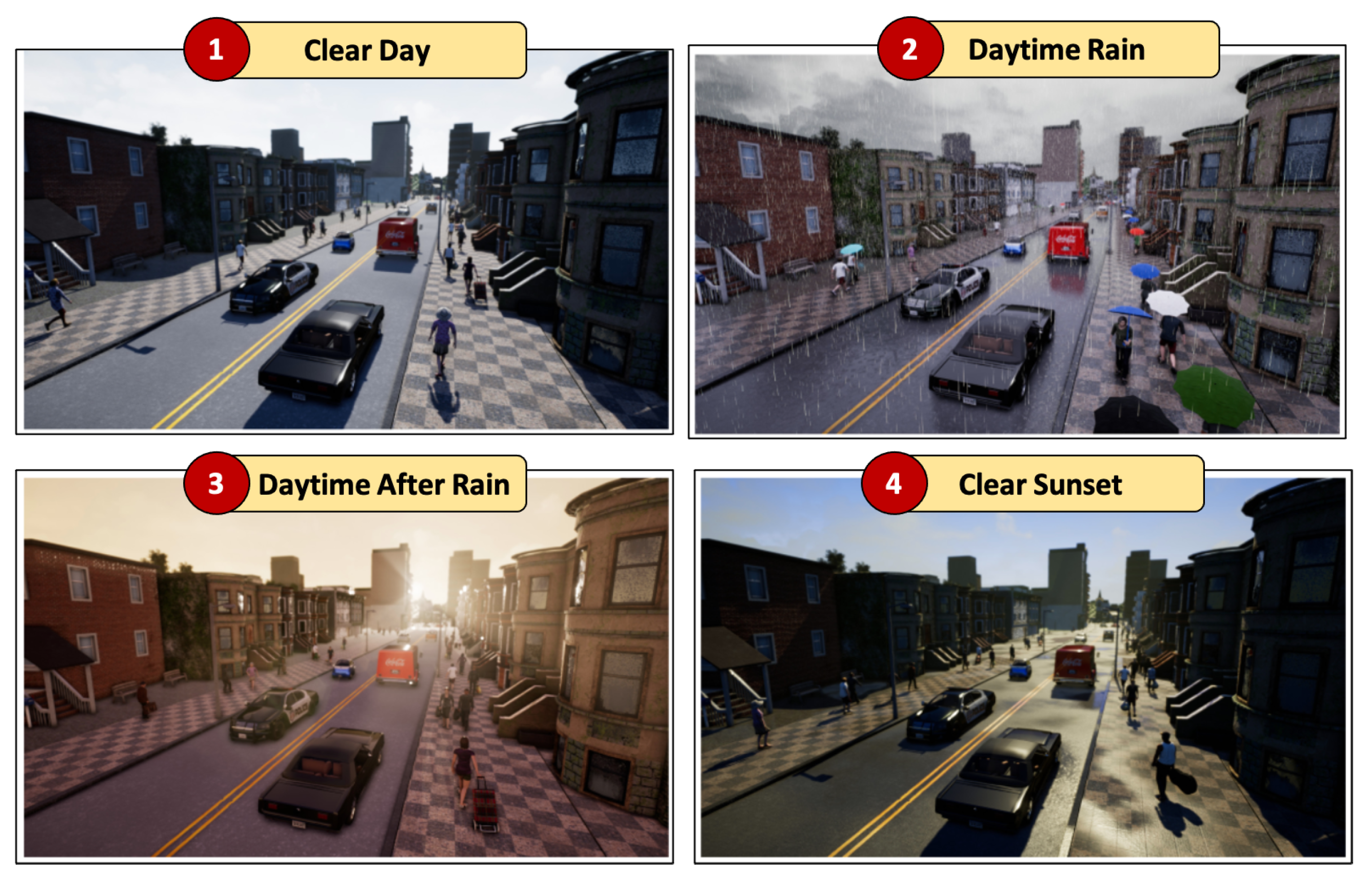
Each town is loaded with suitable weather, which can be customized based on user requirements. Different weather parameters can be set by using the
WeatherParameters class to simulate a particular weather. These parameters are independent of each other, i.e., having more clouds would not automatically result in rain or raining would not automatically create puddles as well. Some of the parameters that can be set are cloudiness, precipitation, wind intensity, fog, sun azimuth, altitude angles, etc. CARLA+ enables the user to validate their solutions in any weather setting. Some of the examples of weather conditions in CARLA are shown in
Figure 3.
4.3. Developing CARLA+
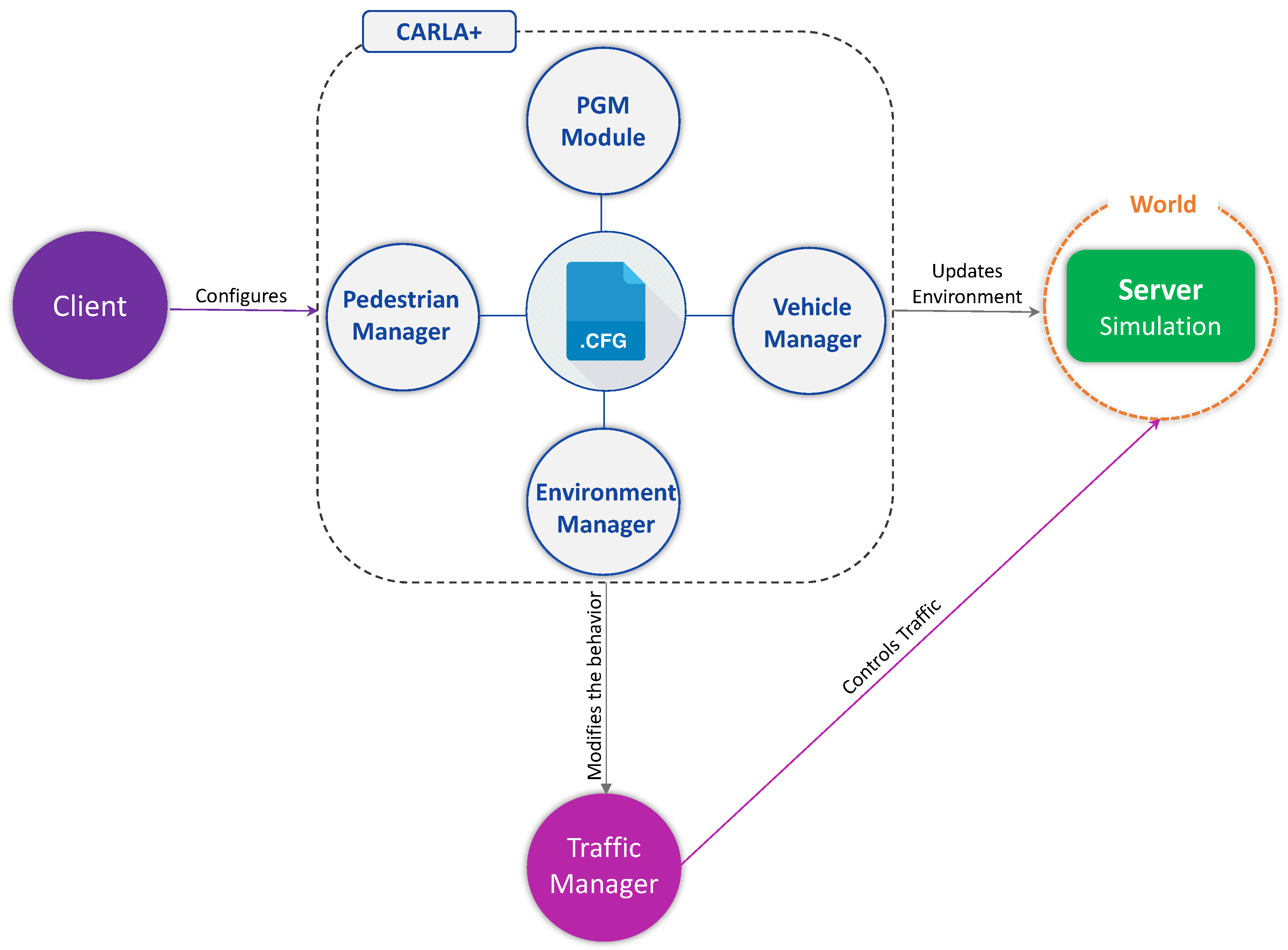
In this section, we discuss the development of CARLA+ and its components. The proposed high-level architecture of CARLA+ is presented in
Figure 4.
The CARLA+ is comprised of four main modules:
Environment Manager Module;
Vehicle Manager Module;
Pedestrian Manager Module;
Integration of PGM Module.
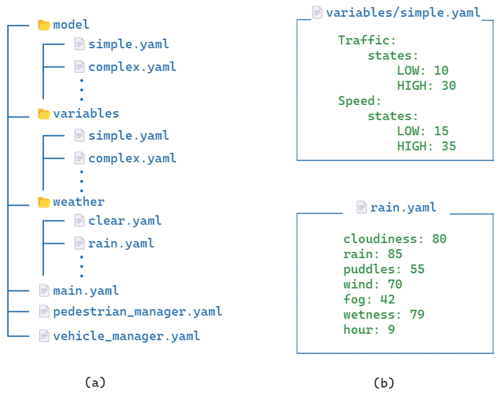
Each of these modules is configured via configuration files, which contain different specifications for environment modeling. The configuration files are an integral piece of the framework as they connect all the other modules together and allow them to function seamlessly. These files are defined in a hierarchical manner where the underlying config can easily be replaced with a different one based on the scenario and requirements.
Figure 5 shows the different configuration files, their folder structure, as well as some sample configs to demonstrate how they are used within CARLA+. Configurations within a particular directory are easily replaceable with another of its peers. For example, to load rainy weather instead of clear, we can easily specify the
weather/rain.yaml file in the main config file. Schema definitions for different types of configurations are also defined to make sure that the user-defined config files conform to the schema definitions. All of these configuration files are modifiable at three levels, i.e., using the actual config files, using the command line, as well as the Python script.
In what follows next, we discuss the functionality and role of each component in detail.
4.3.1. Environment Manager Module
This module deals with the configuration of the simulation environment. It is developed to dynamically simulate the weather and time of day. Based on the provided configuration files, it changes the weather and time inside the simulated environment. It can also dynamically change the weather with the passage of time. The configuration files expose a number of parameters such as cloudiness, rain, wind, fog, etc., where the user can specify the percentage of value required to get the desired weather in the environment. Some of the pre-defined weather configuration files for some common scenarios, such as clear, rainy, cloudy, etc., are also provided. Furthermore, we enable the user to model a particular hour of the day which can automatically be converted into respective sun azimuth and altitude angles to be used in the simulation. All of these configuration files are configurable and can be extended by the researchers allowing for more granular control over every aspect of the simulation environment.
4.3.2. Vehicle Manager Module
This module is developed to adjust the behavior of the traffic inside the simulation. It allows for a wide range of configuration parameters for traffic, such as the number of vehicles to spawn, the maximum allowed speed, the safe distance from the leading vehicle, the type of vehicle to spawn, and more. Each of these parameters can be configured via configuration files and can be modified later on by the PGM model based on the state of the world. The user can also choose to spawn a mixed type of vehicle such as a car, van, truck, etc.
4.3.3. Pedestrian Manager Module
This component is developed to capture the dynamics of the pedestrians in the simulation environment. It manages the number of pedestrians to spawn, and randomly spawns them on various locations around the map. It also provides the functionality to modify the behavior of the spawned pedestrians, such as the percentage of pedestrians that are running or crossing the road, etc. This module can be used to dynamically model the number and behavior of pedestrians in specific scenarios such as roundabouts. We also provide multiple pedestrian models enabling users to spawn various types of pedestrians which can easily be configured via the configuration files provided.
4.3.4. Integrating PGM Module
This is the main component of the CARLA+ that glues all the other components together. It takes the current state of the world as input and predicts the state of different variables based on that. It uses a BN model and loads the Conditional Probability Distribution (CPD) from the configuration files. It then uses the Variable Elimination method to obtain the probability distribution of the required states. The simulated environment is then updated based on the most probable state of the desired variables.
This module is developed to be used in a number of ways. First, the states and CPDs of different variables can be defined entirely in the configuration files manually. The module will create a BN model based on those configuration files. Second, different parameter learning algorithms can be used to directly learn the CPDs of variables from raw data, which can then be exported into the configuration files and loaded into a BN from there. Another approach could be to bypass the configuration files for CPDs and directly load or train the BN when the simulation starts. This flexibility allows us to handle various scenarios, from hand-crafted CPDs to complex CPDs learned directly from real-world data.
Once the model and its CPDs are defined, the CARLA+ loads that model into memory and use that for modeling the simulation. The CARLA client queries the CARLA server for different environmental parameters, and based on the returned parameters, it uses the user-defined PGM model to infer new states for different variables. Once the desired states have been calculated, CARLA+ updates the simulation weather in the CARLA server and traffic count as well as a behavior using the Traffic Manager accordingly. In this way, the CARLA+ framework extends the classical CARLA by integrating it with a PGM framework that is able to model different parameters in the simulated environment and dynamically change the states of those variables based on their dependencies, as defined in the CPD.
Having discussed the design and development of CARLA+, we provide a discussion on clearly highlighting the difference between the classical CARLA and CARLA+. Although CARLA is a comprehensive and well-designed simulator for autonomous driving, providing options to customize the environment including the map, number, and type of vehicles, pedestrians, weather and time of day, automatic and manual traffic control, etc., it does not provide a unified framework to automatically manage those. For instance, we can manually code to spawn a different number of pedestrians based on weather conditions and daytime using multiple conditional statements, but there is no pre-defined way to do so automatically, based on the dynamic simulation environment. Therefore, the proposed CARLA+ takes these different disconnected components of CARLA and provides a unified framework to automate their behaviors leveraging PGMs. For example, a user can define a PGM that models the dynamics of pedestrian counts, vehicle counts, and vehicle speed based on dynamic weather and time of day. CARLA+ is flexible enough and lets the user define the PGM model in different ways: (i) manually defined by the user; (ii) trained on real-world data improving the ability to model different dynamics from the real world. Therefore, instead of manually catering to each condition, CARLA+ enables the user to automate the modeling of different dynamics of the environment. It gives the user more flexibility and control over the dynamic environment, encouraging them to design more complex experimental scenarios.


 ,
, 


