
CARLA+: An Evolution of the CARLA Simulator for Complex Environment Using a Probabilistic Graphical Model

 ,
,  , , , , and
Abstract
:1. Introduction
- Modeling the complex urban environment based on a state-of-art probabilistic graphical model which is suitable for capturing the dynamics specific to urban and higher-level autonomous driving;
- Design and development of an extension of CARLA referred to as CARLA+ by integrating the PGM framework. Instead of manually catering to each condition, it provides a unified framework to automate the behavior of dynamic environments leveraging PGMs;
- Experimentation and validation of the proposed CARLA+ extension.
2. Background
2.1. Autonomous Driving Design Goals
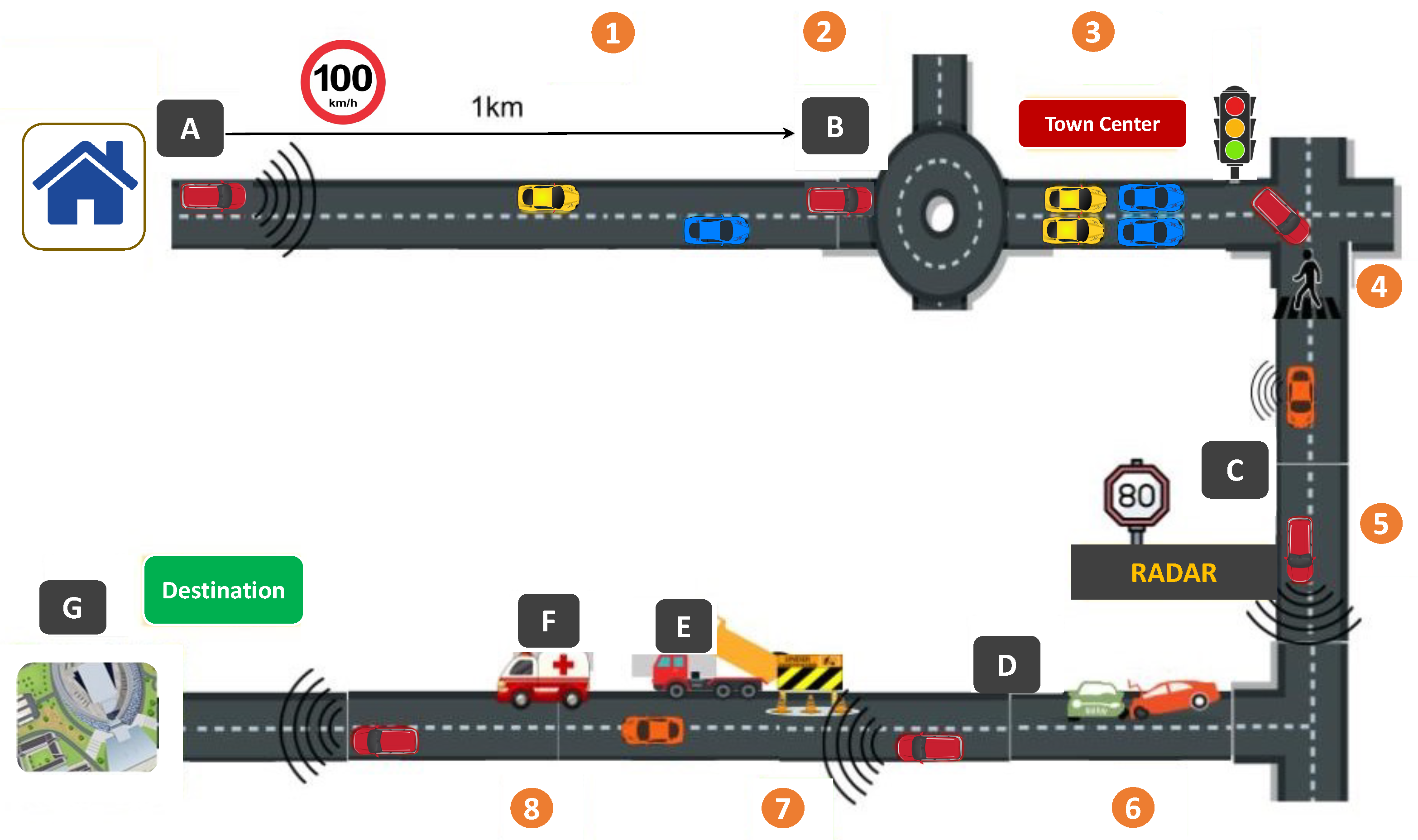
2.2. Complex Dynamics of Urban Environment
3. Related Work
3.1. Autonomous Driving Simulators—An Overview
- MATLAB/Simulink: launched its Automated Driving Toolbox which offers various tools and algorithms to facilitate the design, simulation, and testing of Advanced Driver Assistance Systems (ADAS) and automated driving. It enables the users to test its main functionalities such as environment perception, path planning, and vehicle control. It provides the feature to import HERE HD live map data and OpenDRIVE® road networks into MATLAB and can be used for various design and testing applications. Last but not least, the toolbox allows the development of C/C++ code for faster prototyping and Hardware-in-the-Loop (HIL) testing, providing support for sensor fusion, tracking, path planning, and vehicle controller algorithms.
- PreScan: an open-source physics-based simulation platform that aims to design ADAS and autonomous vehicles. It introduces PreScan’s automated traffic generator, which offers manufacturers a variety of realistic environments and traffic conditions to test their autonomous navigation solutions. It can also be used to design and evaluate V2V and vehicle-to-infrastructure (V2I) communication applications. Among other features, it also provides support for HIL simulation, real-time data, and Global Positioning System (GPS) vehicle data recording, which can then be replayed later. Furthermore, PreScan provides a special function known as the Vehicle Hardware-In-the-Loop (VeHIL) laboratory. The test/ego vehicle is set up on a rolling bench, and other vehicles are represented by wheeled robots that resemble vehicles allowing users to establish a hybrid real-virtual system. Real sensors are installed in the test vehicle. Therefore, the VeHIL is capable of offering thorough simulations for ADAS by utilizing this setup of ego vehicles and mobile robots.
- LGSVL: an open-source multi-robot autonomous driving simulator developed by LG Electronics America R&D Center. It is built on the Unity game Engine and offers various bridges to pass the message between the autonomous driving stack and the simulator backbone. The simulation engine provides different functions to simulate the environment (e.g., traffic simulation and physical environment simulation), sensor simulation, and vehicle dynamics. Additionally, a PythonAPI is available to control various environmental variables, such as the position of the adversaries, the weather, etc. Furthermore, it also provides a Functional Mockup Interface (FMI) to integrate the vehicle dynamics model platform with the external third-party dynamics models. Lastly, exporting high-definition (HD) maps from 3D settings is one of the key capabilities of LGSVL.
- Gazebo: a multi-robot, open-source, scalable, and flexible 3D simulator that enables the simulation of both indoor and outdoor environments. The world and model are the two fundamental elements that make up the 3D scene. The gazebo is comprised of three main libraries which include physics, rendering, and communication library. In addition to these three core libraries, it also provides plugin support that enables the users to communicate with these libraries directly. The gazebo is renowned for its great degree of versatility and its smooth Robot Operating System (ROS) integration. High flexibility has its benefits because it provides users with complete control over the simulation, but it also requires time and effort. In contrast to CARLA and LGSVL simulators, Gazebo requires the user to construct 3D models and precisely specify their physics and location in the simulated world within the XML file. This manual approach is how simulation worlds are created in Gazebo. It provides a variety of sensor models but also allows users to add new ones by using plugins. Moreover, Gazebo is extremely well-liked as a robotic simulator, but the time and effort required to construct intricate and dynamic scenarios prevent it from being the first choice for testing self-driving technology. The gazebo is a standalone simulator but most often it is used with ROS.
- CarSim: a vehicle simulator that is frequently used in both academics and industry. The latest version of it supports moving objects and sensors that are useful for simulations involving ADAS and autonomous vehicles. These moving items, such as vehicles, cyclists, or people, can be connected to 3D objects with their embedded animations. The key advantage of CarSim is that it offers interfaces for other simulators such as MATLAB and LabVIEW. CarSim is not an open-source simulator, but it does have extensive documentation and provides several simulation examples.
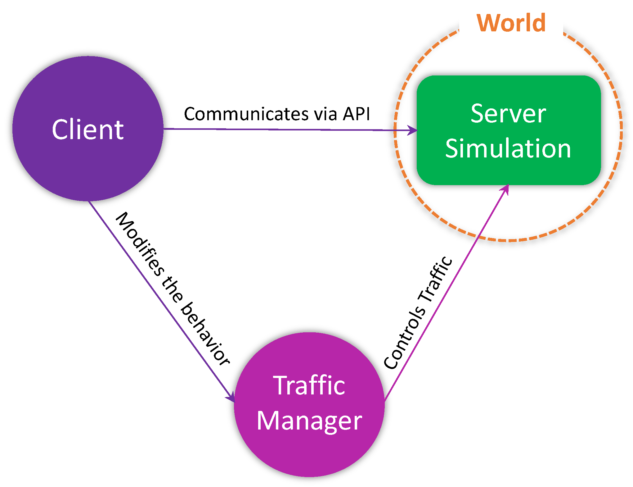
- CARLA [8]: an open-source simulator for autonomous urban driving. It is developed from scratch to support training, prototyping, and validation of autonomous driving solutions including both perception and control. As a result, CARLA makes an effort to meet the needs of different ADAS use cases, such as learning driving rules or training the perception algorithms. It is comprised of a scalable client-server architecture that communicates over transmission control protocol (TCP). It simulates an open, dynamic world implementing an interface between the world and an agent which interacts with the world. The server is responsible for running the simulation, rendering the scenes, sensor rendering, computation of physics, providing the information to the client, etc. Whereas, the client side is comprised of some client modules that aim to control the logic of agents appearing in the scenes. For a detailed discussion on CARLA, the readers are encouraged to look into the authors’ previous publication [9].
3.2. Relevant Studies
4. Proposed Extension to CARLA
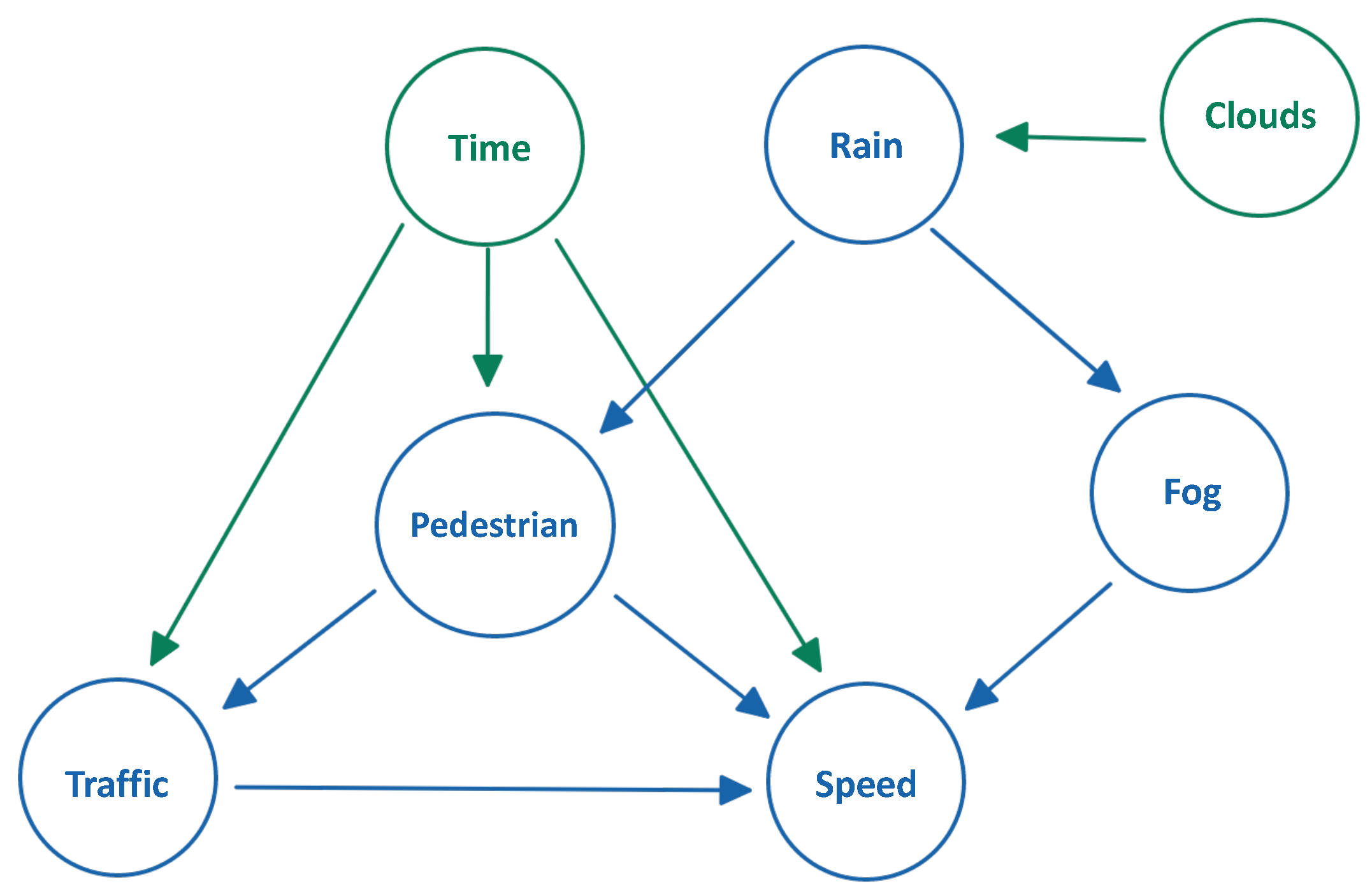
4.1. PGM for Modeling Complex Urban Environment
- It is instrumental in understanding the complex relationship between a set of random variables. This is an important feature because the considered problem domain involves several variables (e.g., number of vehicles, number of pedestrians, vehicle speed, weather state, time of the day, distance from other vehicles and objects, road markings, road signs, road traffic lights, etc.) Furthermore, these variables have an impact on one another, resulting in much more complex interparameter relationships;
- It allows to reuse the knowledge accumulated over the different scenes and settings;
- It allows for solving tasks such as inference learning. This feature is relevant to the considered collaborative autonomous driving problem domain since we are interested in estimating the probability distributions and probability functions in different use cases. For instance, when the probability is associated with the elements of action space in a specific use case, we are interested in achieving the optimal values of the associated probability values;
- It allows the independence properties to represent high-dimensional data more compactly. The independence properties help in the considered problem domain by assisting in understanding the characteristics of a particular attribute separately from the rest of the system;
- The concept of conditional independence brings in significant savings in terms of how to compute and represent the network structure.
| Algorithm 1. Hill-climbing search algorithm for structure learning |
Input: a dataset from X, an empty DAG , a score function Score . Output: the that maximizes the Score .
|
- Tabu List: it first moves away from by allowing up to additional local moves. These moves would generate DAGs with , therefore, the new candidate DAGs would have the highest even though if . Moreover, DAGs accepted as candidates in the last iterations would be saved in a list referred to as the tabu list. It will allow the algorithm to not revisit the recently seen structures aiming to guide the search towards unexplored regions of the space of the DAGs and this approach is referred to as Tabu search.
- Random Restarts: multiple restarts up to r times would allow the algorithm to find the global optimum when at a local optimum.
4.2. Designing CARLA+
4.2.1. CARLA Architecture
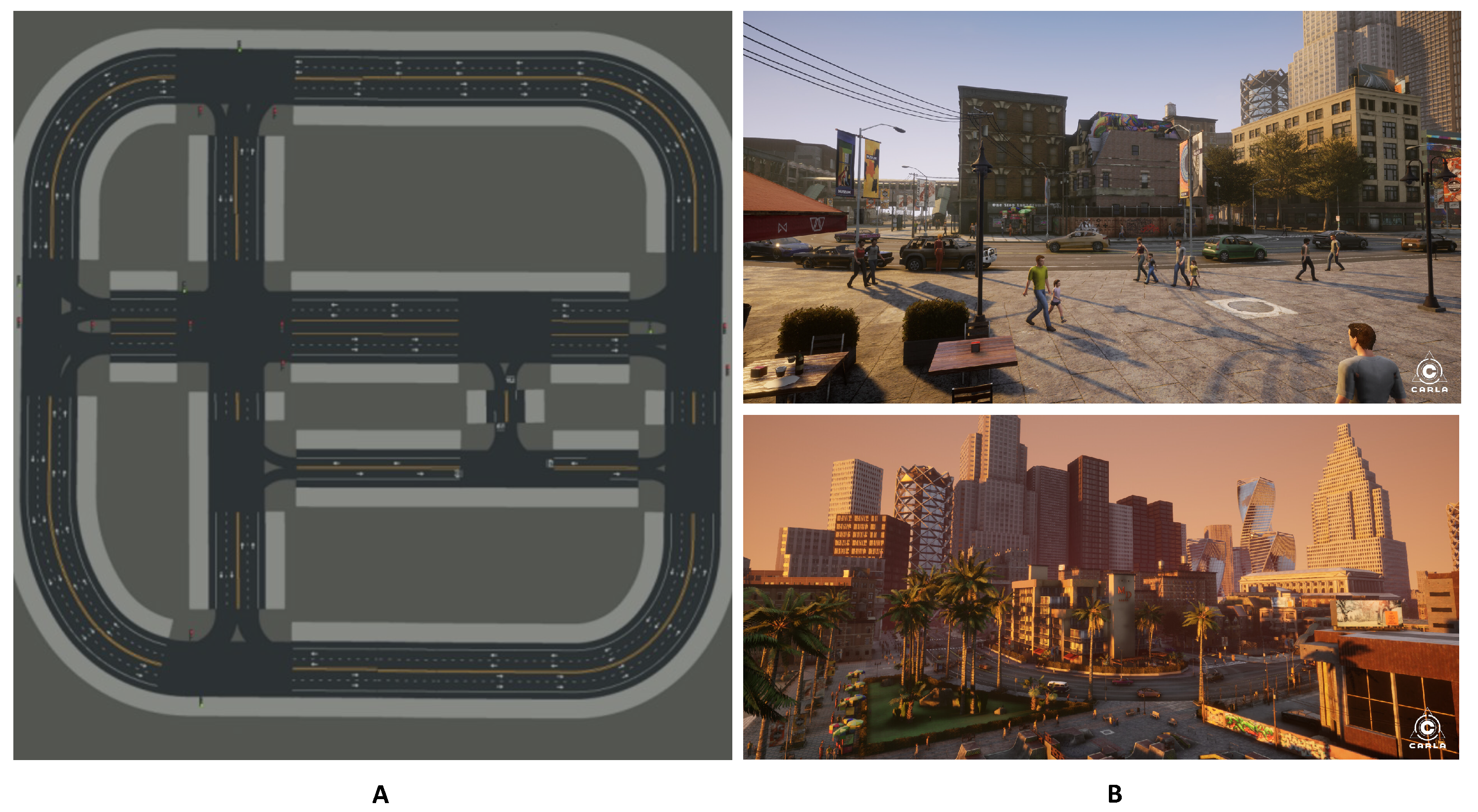
4.2.2. Maps
4.2.3. Vehicles
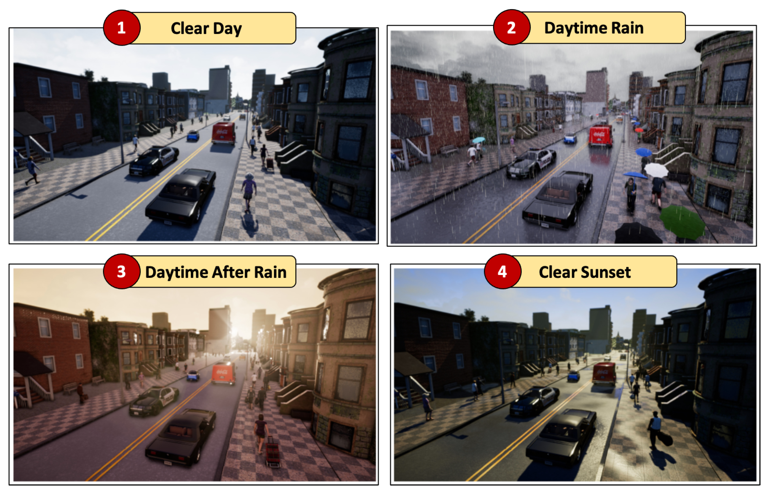
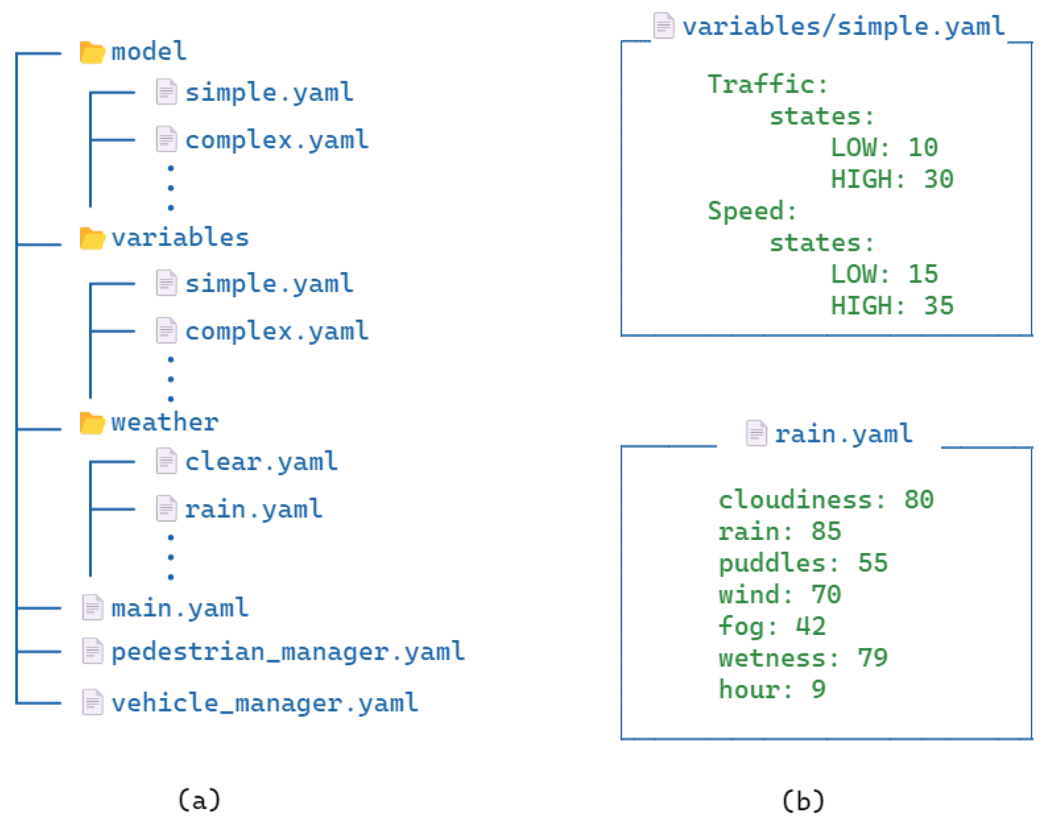
4.2.4. Weather
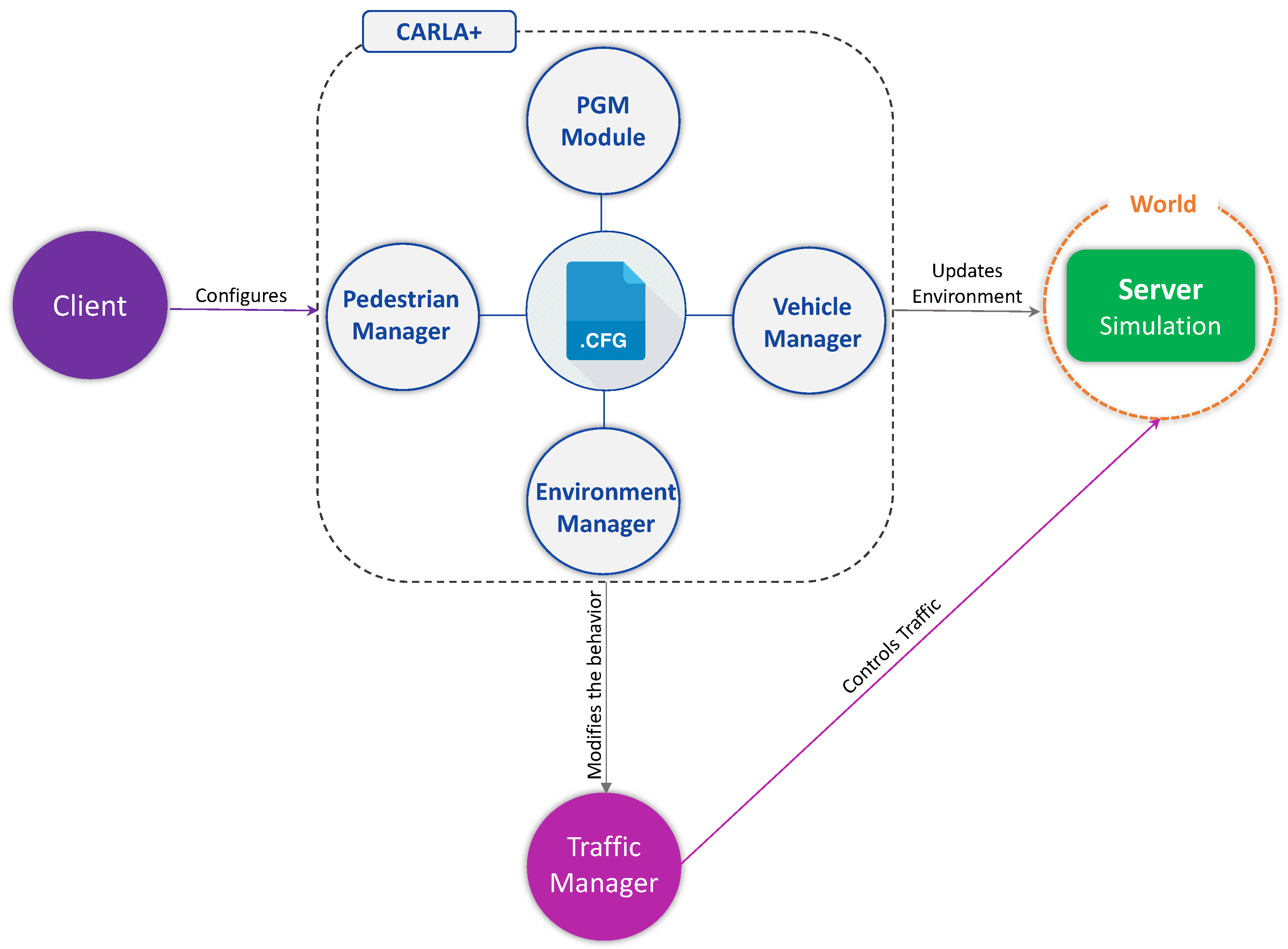
4.3. Developing CARLA+
- Environment Manager Module;
- Vehicle Manager Module;
- Pedestrian Manager Module;
- Integration of PGM Module.
4.3.1. Environment Manager Module
4.3.2. Vehicle Manager Module
4.3.3. Pedestrian Manager Module
4.3.4. Integrating PGM Module
5. Validation of the Proposed CARLA+
5.1. Experimental Setup
5.2. Experiments
5.2.1. Controlled Settings
5.2.2. Learning-Based Settings
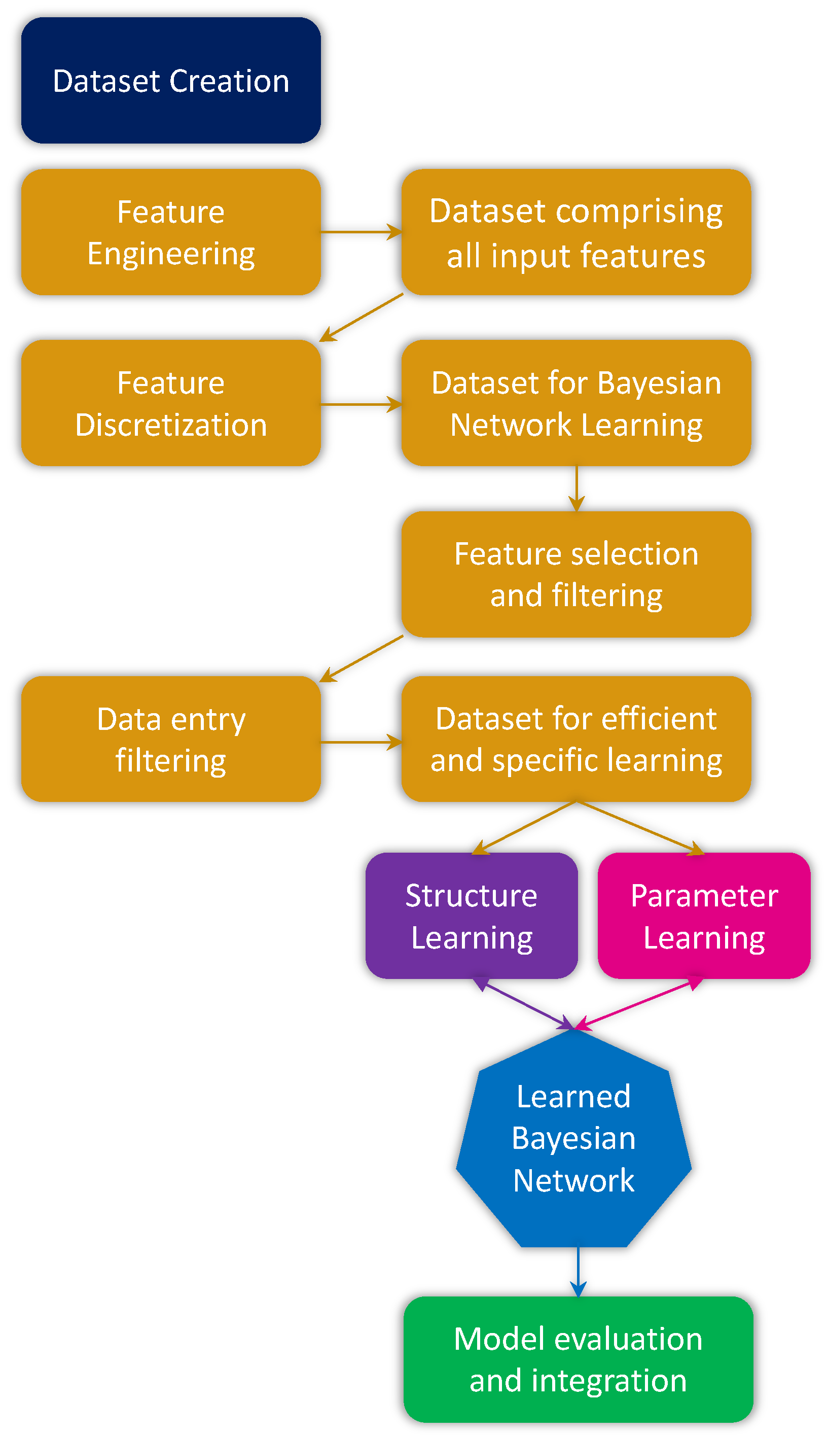
Dataset Creation
- Traffic Count: for the traffic count, we used New York City’s open data platform [20] which contains data for traffic volume counts. It contains traffic volume data of different streets in the boroughs of New York City, taken at 15-minute intervals.
- Pedestrian Count: for pedestrians counts, we used the Brooklyn Bridge Automated Pedestrian Counts data [21], which contains pedestrian count as well as basic weather data, taken at 1-hour intervals.
- Traffic Speed: we used New York City’s Real-Time Traffic Speed data [22] which is comprised of the traffic speed as well as the borough where the data were captured.
- Weather: the NYC weather data are taken from Open-Meteo’s Historical Weather API [23] for the city of Brooklyn.
Data Preparation and Feature Engineering
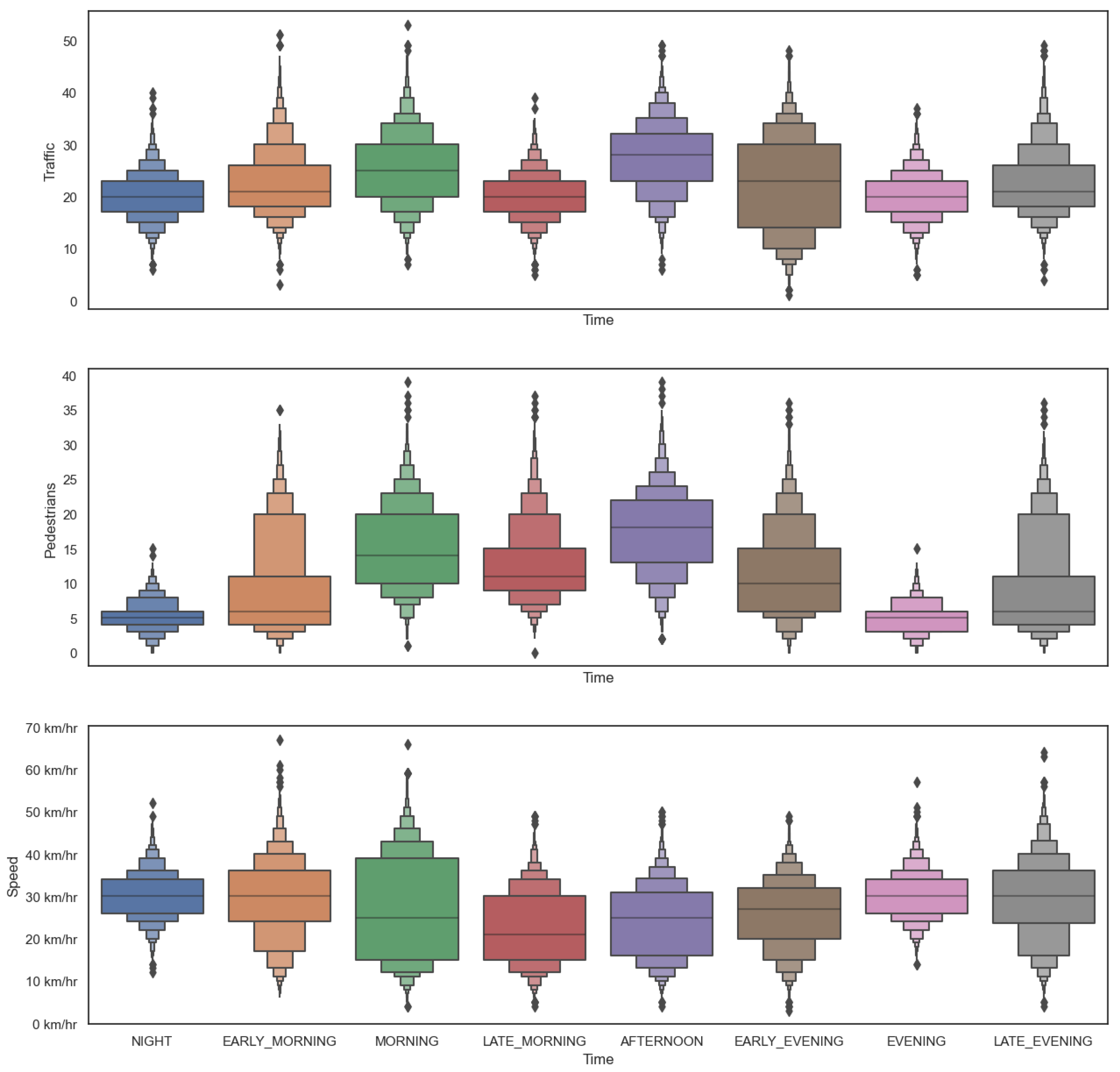
- Hour
- Pedestrians
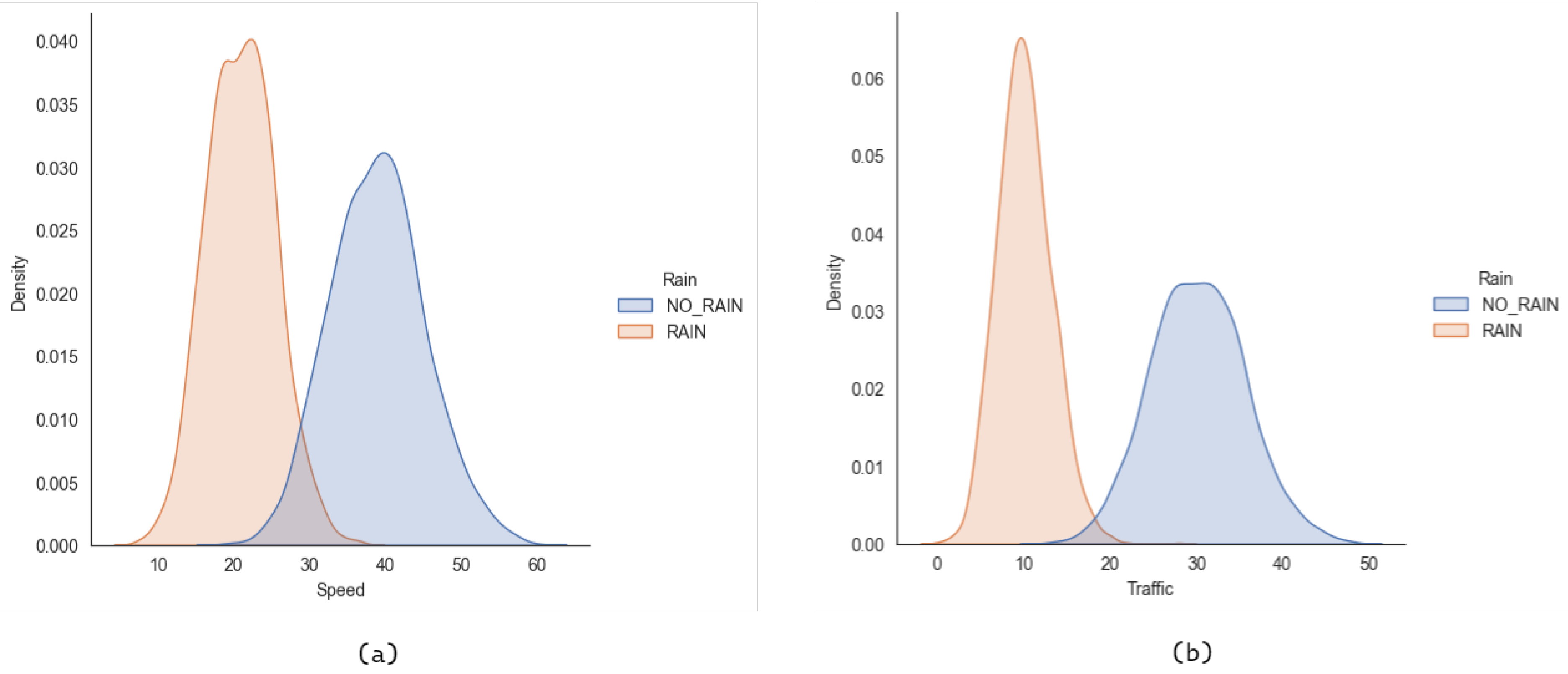
- Traffic
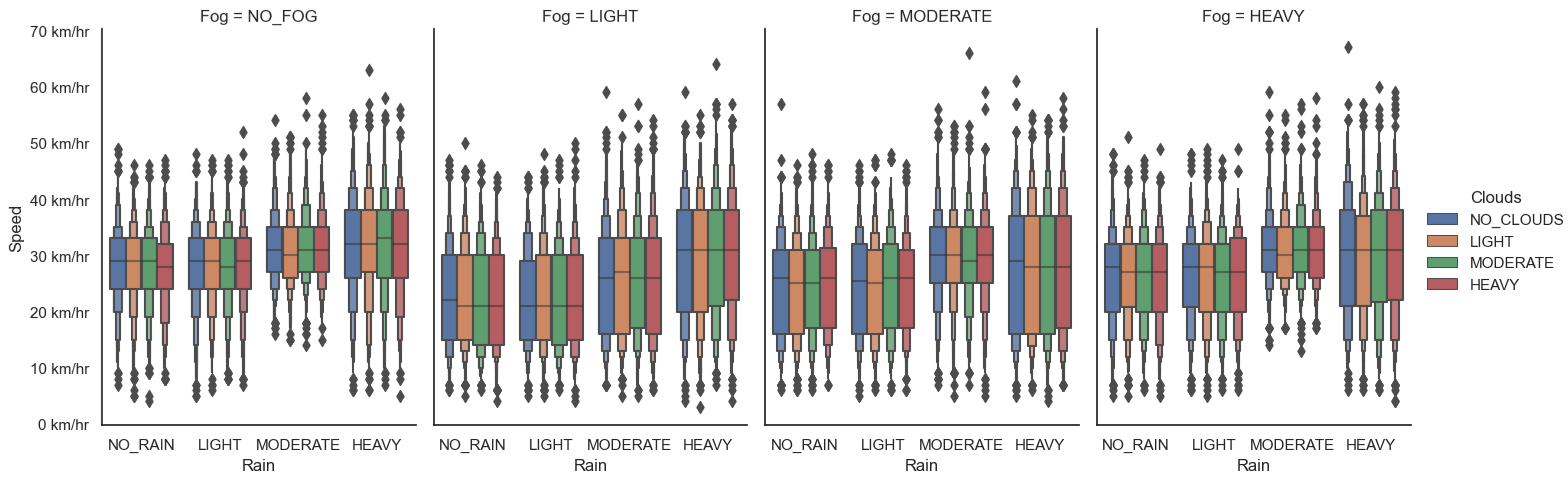
- Speed
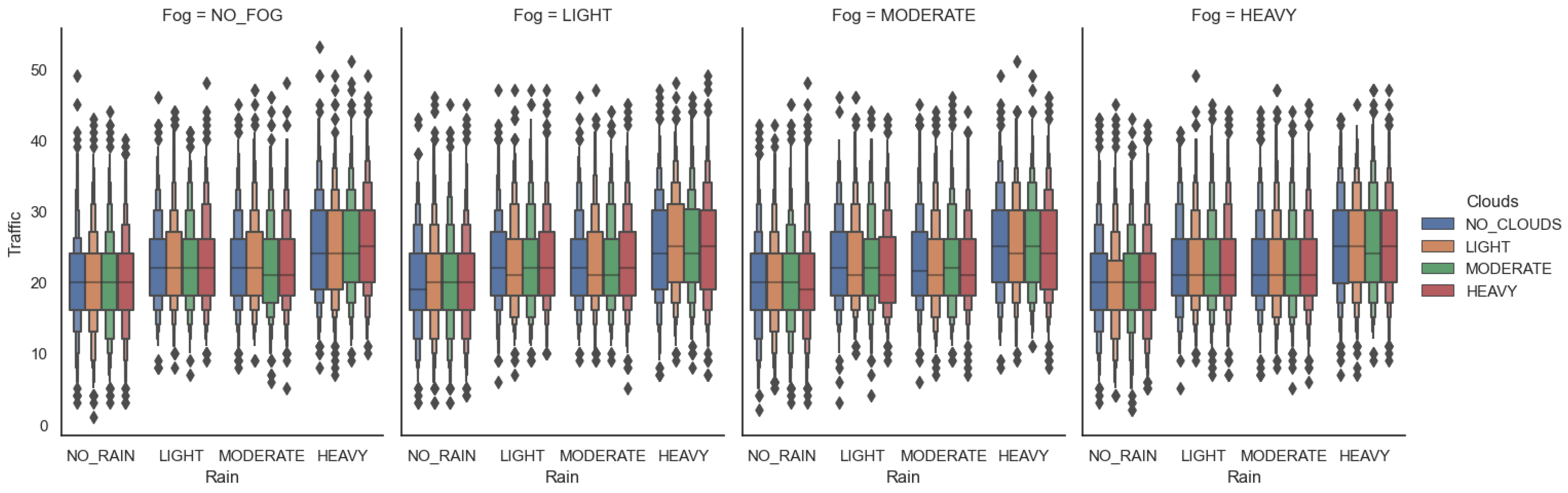
- Rain
- Fog
- Clouds
Learning and Integration of PGM Model
6. Conclusions
Author Contributions
Funding
Institutional Review Board Statement
Informed Consent Statement
Data Availability Statement
- The open-source code of CARLA+ is available at https://github.com/aadimator/CARLA-Plus (accessed on 2 January 2023)
- The processed and discretized Traffic dataset is available at https://www.kaggle.com/datasets/aadimator/brooklyn-2019-traffic-data (accessed on 2 January 2023)
Conflicts of Interest
Abbreviations
| 3GPP | 3rd Generation Partnership Project |
| ACC | Adaptive Cruise Control |
| AD | Autonomous Driving |
| ADAS | Advanced Driving Assistance Systems |
| AV | Autonomous Vehicle |
| BN | Bayesian Network |
| CACC | Cooperative Adaptive Cruise Control |
| CPD | Conditional Probability Distribution |
| CARLA | Car Learning to Act |
| DAG | Directed Acyclic Graph |
| HC | Hill Climbing |
| PGM | Probabilistic Graphical Model |
| ROS | Robot Operating System |
| SAE | Society of Automotive Engineers |
| V2I | Vehicle-to-Infrastructure |
| V2V | Vehicle-to-Vehicle |
| V2X | Vehicle-to-Everything |
References
- Batkovic, I. Enabling Safe Autonomous Driving in Uncertain Environments. Ph.D. Thesis, Chalmers Tekniska Hogskola, Goteborg, Sweden, 2022. [Google Scholar]
- SAE Levels of Driving AutomationTM Refined for Clarity and International Audience. Available online: https://www.sae.org/blog/sae-j3016-update (accessed on 20 December 2022).
- Baltodano, S.; Sibi, S.; Martelaro, N.; Gowda, N.; Ju, W. RRADS: Real road autonomous driving simulation. In Proceedings of the Tenth Annual ACM/IEEE International Conference on Human-Robot Interaction Extended Abstracts, Portland, OR, USA, 2–5 March 2015; p. 283. [Google Scholar]
- Udacity Universe | Udacity. Available online: https://www.udacity.com/universe (accessed on 17 October 2022).
- 3GPP—The Mobile Broadband Standard Partnership Project. Available online: https://www.3gpp.org/ (accessed on 17 October 2022).
- Khan, M.J.; Khan, M.A.; Beg, A.; Malik, S.; El-Sayed, H. An overview of the 3GPP identified Use Cases for V2X Services. Procedia Comput. Sci. 2022, 198, 750–756. [Google Scholar] [CrossRef]
- Malik, S.; Khan, M.A.; El-Sayed, H. Collaborative autonomous driving—A survey of solution approaches and future challenges. Sensors 2021, 21, 3783. [Google Scholar] [CrossRef] [PubMed]
- Dosovitskiy, A.; Ros, G.; Codevilla, F.; Lopez, A.; Koltun, V. CARLA: An open urban driving simulator. In Proceedings of the Conference on Robot Learning, Mountain View, CA, USA, 13–15 November 2017; pp. 1–16. [Google Scholar]
- Malik, S.; Khan, M.A.; El-Sayed, H. CARLA: Car Learning to Act—An Inside Out. Procedia Comput. Sci. 2022, 198, 742–749. [Google Scholar] [CrossRef]
- Gómez-Huélamo, C.; Egido, J.D.; Bergasa, L.M.; Barea, R.; López-Guillén, E.; Arango, F.; Araluce, J.; López, J. Train here, drive there: Simulating real-world use cases with fully-autonomous driving architecture in carla simulator. In Proceedings of the Workshop of Physical Agents, Madrid, Spain, 19–20 November 2020; pp. 44–59. [Google Scholar]
- Gómez-Huélamo, C.; Del Egido, J.; Bergasa, L.M.; Barea, R.; López-Guillén, E.; Arango, F.; Araluce, J.; López, J. Train here, drive there: ROS based end-to-end autonomous-driving pipeline validation in CARLA simulator using the NHTSA typology. Multimed. Tools Appl. 2022, 81, 4213–4240. [Google Scholar] [CrossRef]
- Ramakrishna, S.; Luo, B.; Kuhn, C.; Karsai, G.; Dubey, A. ANTI-CARLA: An Adversarial Testing Framework for Autonomous Vehicles in CARLA. arXiv 2022, arXiv:2208.06309. [Google Scholar]
- Reich, J.; Trapp, M. SINADRA: Towards a framework for assurable situation-aware dynamic risk assessment of autonomous vehicles. In Proceedings of the 2020 16th European Dependable Computing Conference (EDCC), Munich, Germany, 7–10 September 2020; pp. 47–50. [Google Scholar]
- Majumdar, R.; Mathur, A.; Pirron, M.; Stegner, L.; Zufferey, D. Paracosm: A test framework for autonomous driving simulations. In Proceedings of the International Conference on Fundamental Approaches to Software Engineering, Luxembourg, 27 March–1 April 2021; pp. 172–195. [Google Scholar]
- Vukić, M.; Grgić, B.; Dinčir, D.; Kostelac, L.; Marković, I. Unity based urban environment simulation for autonomous vehicle stereo vision evaluation. In Proceedings of the 2019 42nd International Convention on Information and Communication Technology, Electronics and Microelectronics (MIPRO), Opatija, Croatia, 20–24 May 2019; pp. 949–954. [Google Scholar]
- Teper, H.; Bayuwindra, A.; Riebl, R.; Severino, R.; Chen, J.J.; Chen, K.H. AuNa: Modularly Integrated Simulation Framework for Cooperative Autonomous Navigation. arXiv 2022, arXiv:2207.05544. [Google Scholar]
- Cai, P.; Lee, Y.; Luo, Y.; Hsu, D. Summit: A simulator for urban driving in massive mixed traffic. In Proceedings of the 2020 IEEE International Conference on Robotics and Automation (ICRA), Paris, France, 31 May–31 August 2020; pp. 4023–4029. [Google Scholar]
- Kiyak, E.; Unal, G. Small aircraft detection using deep learning. Aircr. Eng. Aerosp. Technol. 2021, 93, 671–681. [Google Scholar] [CrossRef]
- Unal, G. Visual target detection and tracking based on Kalman filter. J. Aeronaut. Space Technol. 2021, 14, 251–259. [Google Scholar]
- Automated Traffic Volume Counts | NYC Open Data. Available online: https://data.cityofnewyork.us/Transportation/Automated-Traffic-Volume-Counts/7ym2-wayt (accessed on 14 November 2022).
- Brooklyn Bridge Automated Pedestrian Counts Demonstration Project | NYC Open Data. Available online: https://data.cityofnewyork.us/Transportation/Brooklyn-Bridge-Automated-Pedestrian-Counts-Demons/6fi9-q3ta (accessed on 14 November 2022).
- Real-Time Traffic Speed Data | NYC Open Data. Available online: https://data.cityofnewyork.us/Transportation/Real-Time-Traffic-Speed-Data/qkm5-nuaq (accessed on 14 November 2022).
- Historical Weather API | Open-Meteo.com. Available online: https://open-meteo.com/en/docs/historical-weather-api/#latitude=&longitude=&start_date=2016-01-01%5C&end_date=2022-10-25%5C&hourly=precipitation,rain,cloudcover (accessed on 14 November 2022).


| SAE Level of Automation | Testing Requirements | ||
|---|---|---|---|
| Level (L) | Description | Example | |
| L0 | No Automation: There should always be a human driver in the vehicle performing the dynamic driving task. Only warnings and temporary assistance are offered as features. | Blind spot warning | Simulation of traffic flow, multiple road types, radar and camera sensors |
| L1 | Driver Assistance: It is necessary to have a driver at all times. Steering or brake/acceleration control is provided through features. | Adaptive Cruise Control (ACC) & Lane centering | All of the above (AoB) in addition to simulation of vehicle dynamics and ultrasonic sensors |
| L2 | Partial Driving Automation: the system is in charge of longitudinal and lateral vehicle motion within a constrained operational design domain. Features include both steering and brake/acceleration control. | ACC & lane centering at the same time. | AoB and the simulation of a driver monitoring system and machine–human interaction |
| L3 | Conditional Automation: in case of any failure, the system can request the human intervention. | Traffic Jam Chauffer | AoB and the simulation of traffic infrastructure and dynamic objects |
| L4 | High Automation: the automated driving system is in charge of detecting, observing, and reacting to events. Features can operate the vehicle in a few limited scenarios. | High Driving Automation | AoB and simulations of various weather conditions, lidar, camera, and radar sensors, mapping, and localization |
| L5 | Full Automation: L5 AVs will be able to navigate through complicated environments and deal with unforeseen circumstances without human interaction. | Robo-Taxi | All of the above, along with adhering to all traffic laws, norms, and V2X communication |
| Features | Simulator | ||||||||
|---|---|---|---|---|---|---|---|---|---|
| CARLA | AirSim | DeepDrive | LGSVL | NVIDIA Drive | rFpro | MATLAB | Gazebo | ||
| General | Licence | Open-Source | Open-Source | Open Source | Open-Source | Commercial | Commercial | Commercial | Open-Source |
| Portability | Windows and Linux | Windows and Linux | Windows and Linux | Windows and Linux | Windows and Linux | Windows and Linux | Windows and Linux | Windows and Linux | |
| Physics Engine | Unreal Engine | Unreal Engine and Unity | Unreal Engine | Unity | Unreal Engine | U | Unreal Engine | DART | |
| Scripting Languages | Python | C++, Python, Java | C++, Python | Python | Python | U | MATLAB | C++, Python | |
| Environmental | Urban Driving | Town | Town, City | Road Track | City | City, Harbor | Town, City, Road Track | N | Road Track |
| Off-Road | N | Forest, Mountain | N | N | N | N | N | N | |
| Actors–Human | Y | N | N | Y | N/A | Y | Y | Y | |
| Actors–Cars | Y | Y | Y | Y | N/A | Y | Y | Y | |
| Weather Conditions | Y | Y | Y | Y | Y | Y | N | N | |
| Sensors | RGB | Y | Y | Y | Y | Y | Y | Y | Y |
| Depth | Y | Y | Y | Y | N/A | Y | N | N | |
| Thermal | N | Y | N | N | N/A | N/A | N | Y | |
| LiDAR | Y | Y | N | Y | Y | Y | Y | Y | |
| RADAR | Y | N | N | Y | Y | Y | Y | Y | |
| Output Training Labels | Semantic Segmentation | Y | Y | N | Y | Y | Y | Y | Y |
| 2D Bounding Box | Y | N | N | Y | Y | N/A | Y | Y | |
| 3D Bounding Box | Y | N | Y | Y | N/A | N/A | Y | Y | |
| Requirement | Version | Usage |
|---|---|---|
| Operating Sysyem | Windows 11 | - |
| RAM | 16 GB | - |
| CPU | Intel i7 | - |
| GPU | NVIDIA GTX 1080 | - |
| CARLA | v0.9.13 | To simulate the environment |
| Python | v3.7 | Scripting language |
| Pgmpy | v0.1.19 | For Bayesian networks |
| Hydra | v1.2.0 | For configuration management |
| Scikit-learn | v1.0.2 | For data analysis |
| Matplotlib | v3.6.2 | For plotting |
| Random Variable | States | |
|---|---|---|
| Rain | NO_RAIN | RAIN |
| Traffic | LOW | HEAVY |
| Speed | LOW | HIGH |
| Hour Classification into Time of the Day | |
|---|---|
| 2:00 AM to 6:00 AM | Early Morning |
| 6:00 AM to 9:00 AM | Morning |
| 9:00 AM to 12:00 | Late Morning |
| 12:00 PM to 5:00 PM | Afternoon |
| 5:00 PM to 7:00 PM | Eary Evening |
| 7:00 PM to 9:00 PM | Evening |
| 9:00 PM to 11:00 PM | Late Evening |
| 11:00 PM to 2:00 AM | Night |
| Label | Rain (mm/h) | Fog (%) | Clouds (%) |
|---|---|---|---|
| NO | 0 | 0–25 | 0–25 |
| LIGHT | 0.1–2.5 | 25–50 | 25–50 |
| MODERATE | 2.6–7.5 | 50–75 | 50–75 |
| HEAVY | >7.5 | 75–100 | 75–100 |
| Label | Traffic | Pedestrian | Speed (km/h) |
|---|---|---|---|
| LOW | 0–200 | 0–100 | 0–30 |
| MEDIUM | 200–800 | 100–1200 | 30–45 |
| HIGH | >800 | >1200 | 45–55 |
| Learning Stage | Parameter | Value |
|---|---|---|
| Structure Learning | Scoring method | k2score |
| Epsilon | 1 × 10 | |
| White list | Possible edges | |
| Parameter Learning | Estimator | BayesianEstimator |
| Prior type | BDeu | |
| Equivalent sample size | 10 | |
| Complete samples only | FALSE |
Disclaimer/Publisher’s Note: The statements, opinions and data contained in all publications are solely those of the individual author(s) and contributor(s) and not of MDPI and/or the editor(s). MDPI and/or the editor(s) disclaim responsibility for any injury to people or property resulting from any ideas, methods, instructions or products referred to in the content. |
© 2023 by the authors. Licensee MDPI, Basel, Switzerland. This article is an open access article distributed under the terms and conditions of the Creative Commons Attribution (CC BY) license (https://creativecommons.org/licenses/by/4.0/).
Share and Cite
Malik, S.; Khan, M.A.; Aadam; El-Sayed, H.; Iqbal, F.; Khan, J.; Ullah, O. CARLA+: An Evolution of the CARLA Simulator for Complex Environment Using a Probabilistic Graphical Model. Drones 2023, 7, 111. https://doi.org/10.3390/drones7020111
Malik S, Khan MA, Aadam, El-Sayed H, Iqbal F, Khan J, Ullah O. CARLA+: An Evolution of the CARLA Simulator for Complex Environment Using a Probabilistic Graphical Model. Drones. 2023; 7(2):111. https://doi.org/10.3390/drones7020111
Chicago/Turabian StyleMalik, Sumbal, Manzoor Ahmed Khan, Aadam, Hesham El-Sayed, Farkhund Iqbal, Jalal Khan, and Obaid Ullah. 2023. "CARLA+: An Evolution of the CARLA Simulator for Complex Environment Using a Probabilistic Graphical Model" Drones 7, no. 2: 111. https://doi.org/10.3390/drones7020111
APA StyleMalik, S., Khan, M. A., Aadam, El-Sayed, H., Iqbal, F., Khan, J., & Ullah, O. (2023). CARLA+: An Evolution of the CARLA Simulator for Complex Environment Using a Probabilistic Graphical Model. Drones, 7(2), 111. https://doi.org/10.3390/drones7020111