

An Intelligent Fault Diagnosis Approach for Multirotor UAVs Based on Deep Neural Network of Multi-Resolution Transform Features


Abstract
1. Introduction
- Stating the main drawbacks in recently published studies on multirotor UAVs’ condition monitoring.
- The implementation of a hybrid signal processing-based discrete wavelet transform and a deep neural network model of an original-equation-derived structure to observe UAV vibration signals.
- Quantifying the probability of defects and pre-failure situations over a long period to create a convenient accumulated depiction of specifications considering the cumulative fault impact.
- Presenting a versatile and risk-free experimental methodology in acquiring vibration signals of any multirotor UAV.
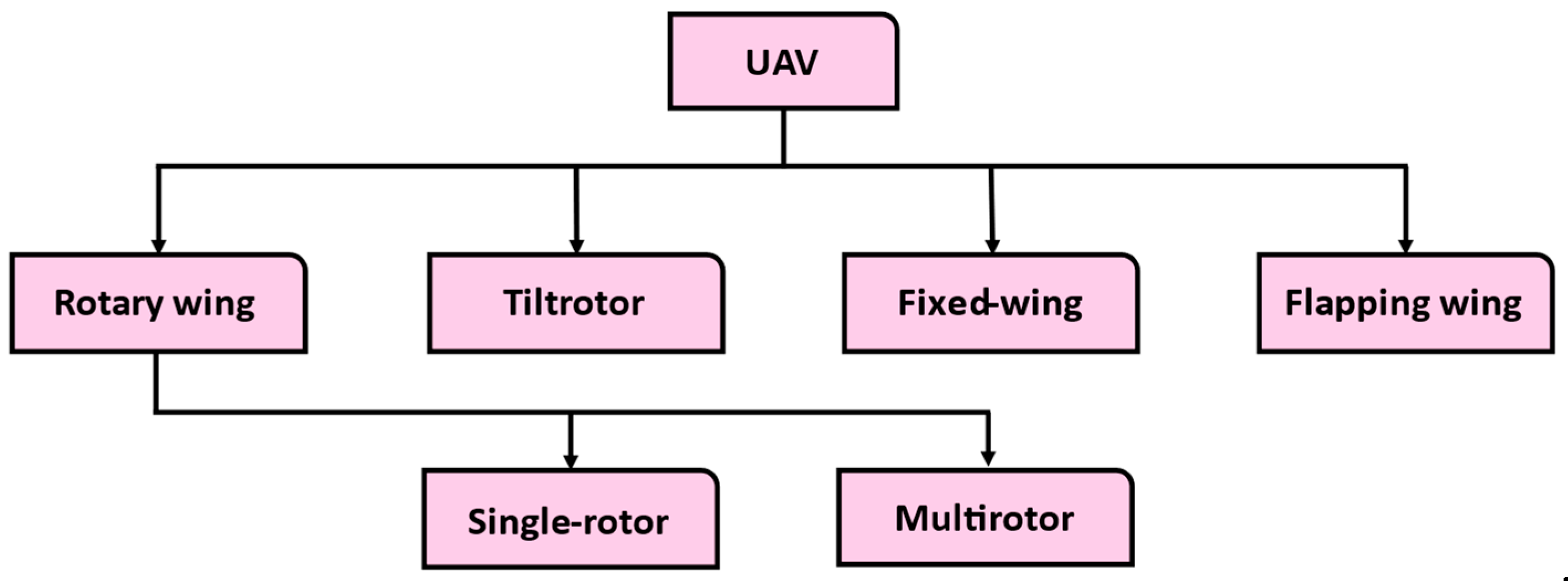
2. UAV and Multirotor UAV Faults’ Classification
2.1. Sensor Faults
2.2. Actuator Faults
3. Theoretical Basis
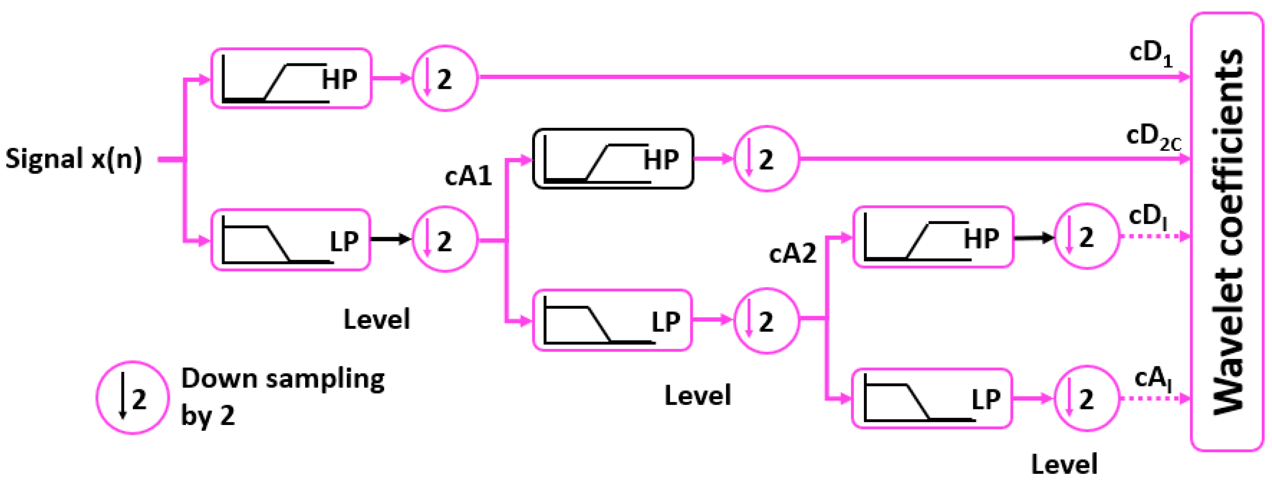
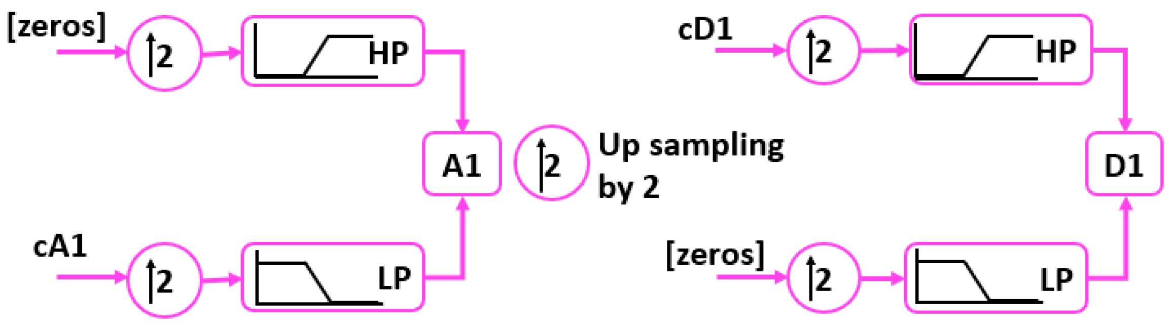
3.1. Discrete Wavelet Transform
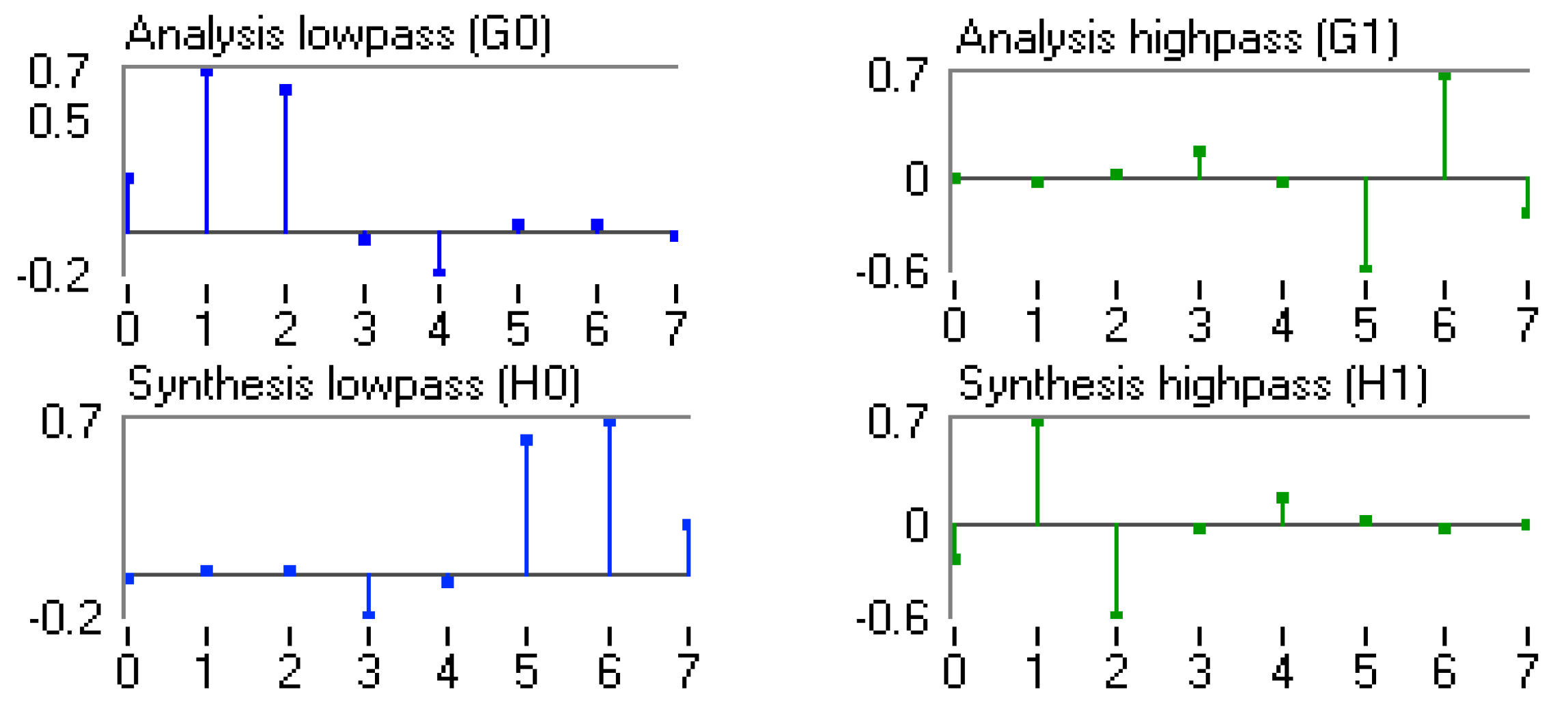
3.2. Selection of the Optimum Mother Wavelet
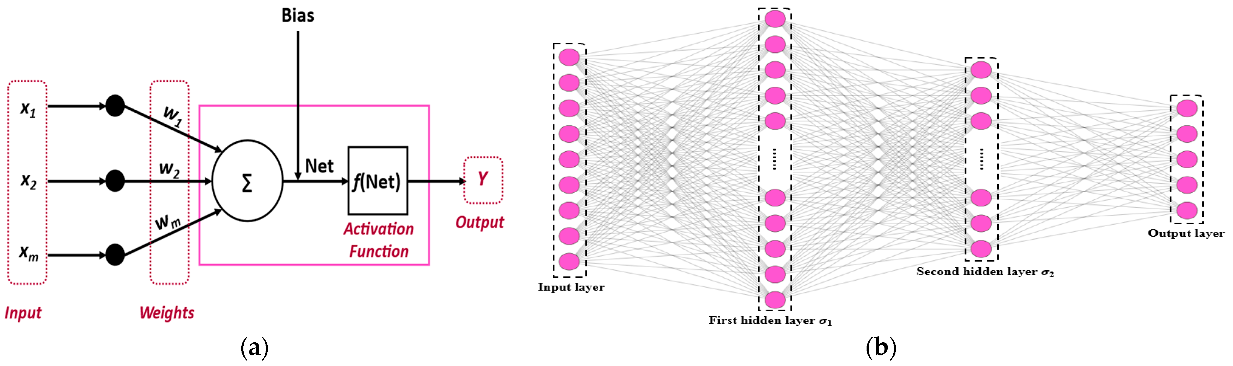
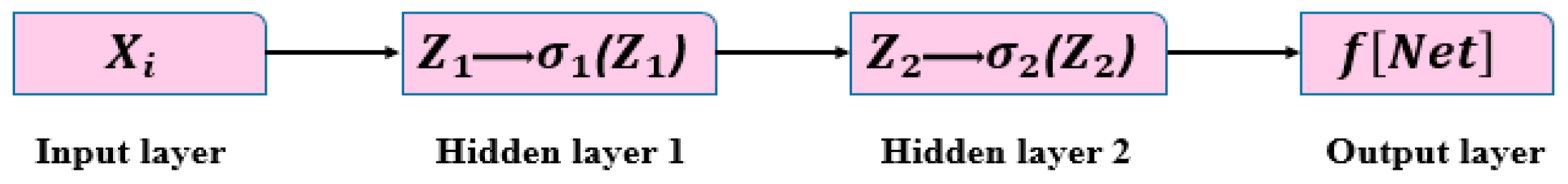
3.3. Deep Neural Network
4. The Experimental Approach
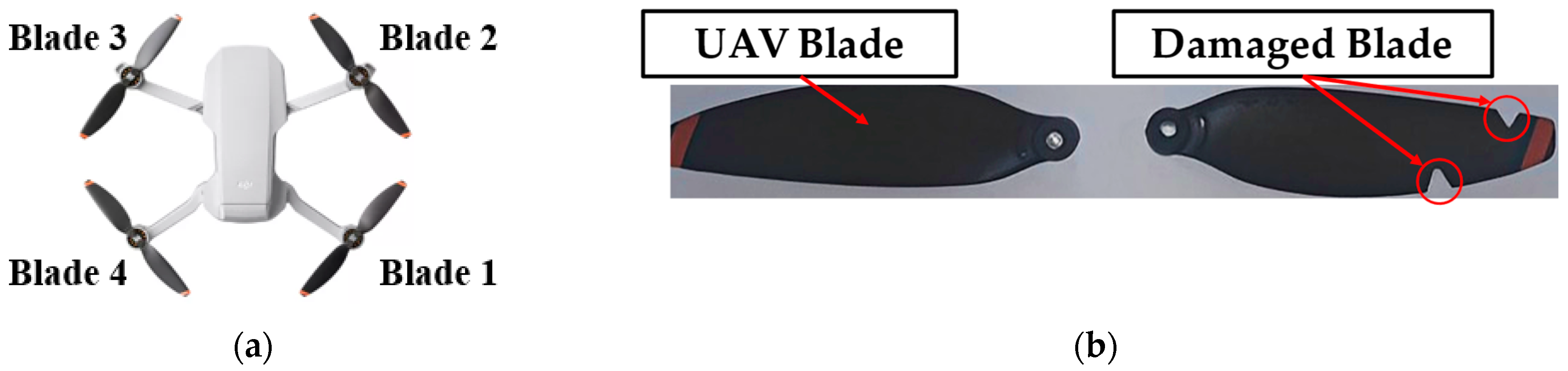
4.1. Drone Selection
4.2. Accelerometer Selection
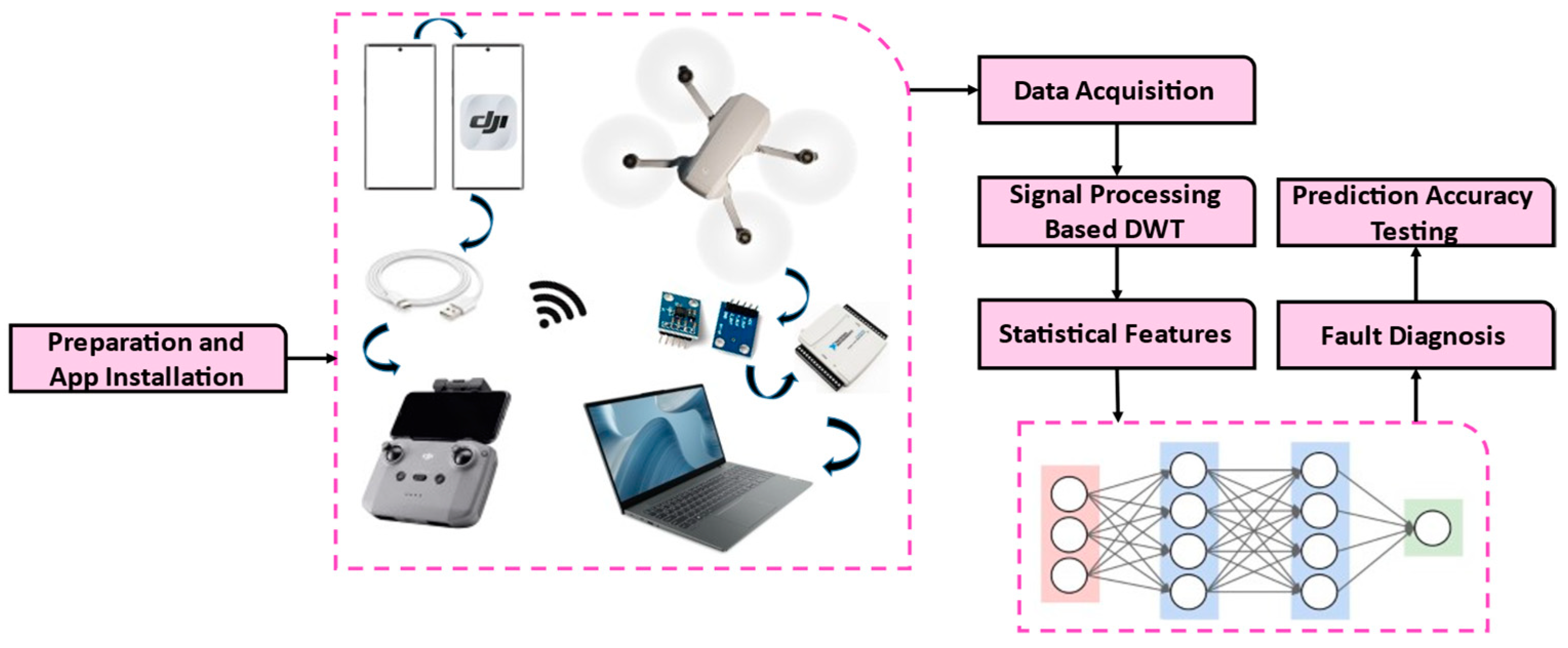
4.3. Methodology
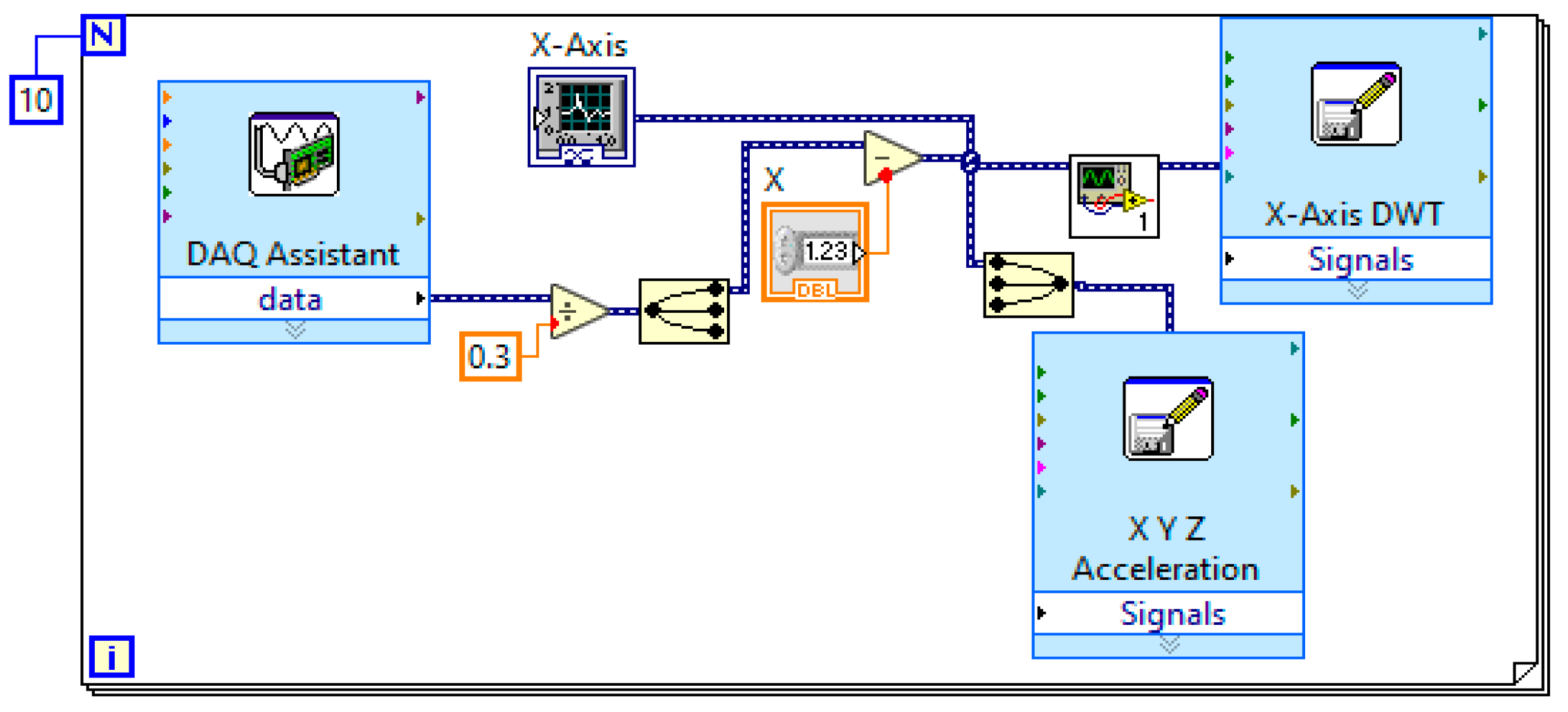
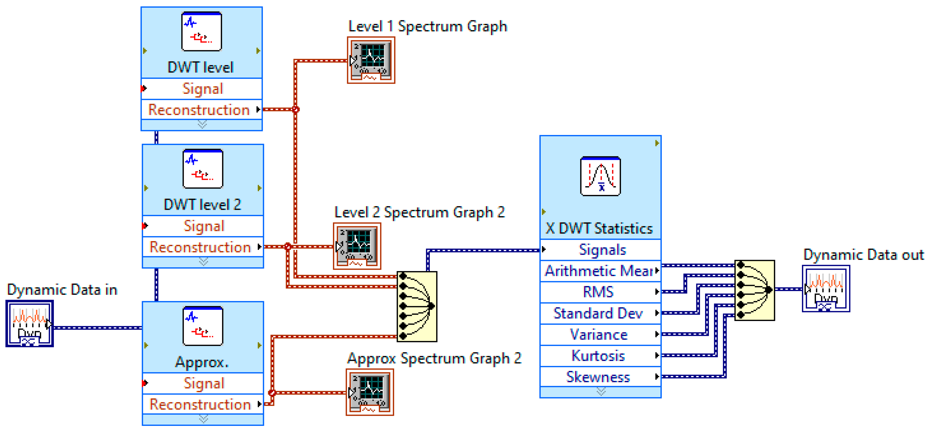
4.4. The Developed LabVIEW Program for Signal Processing
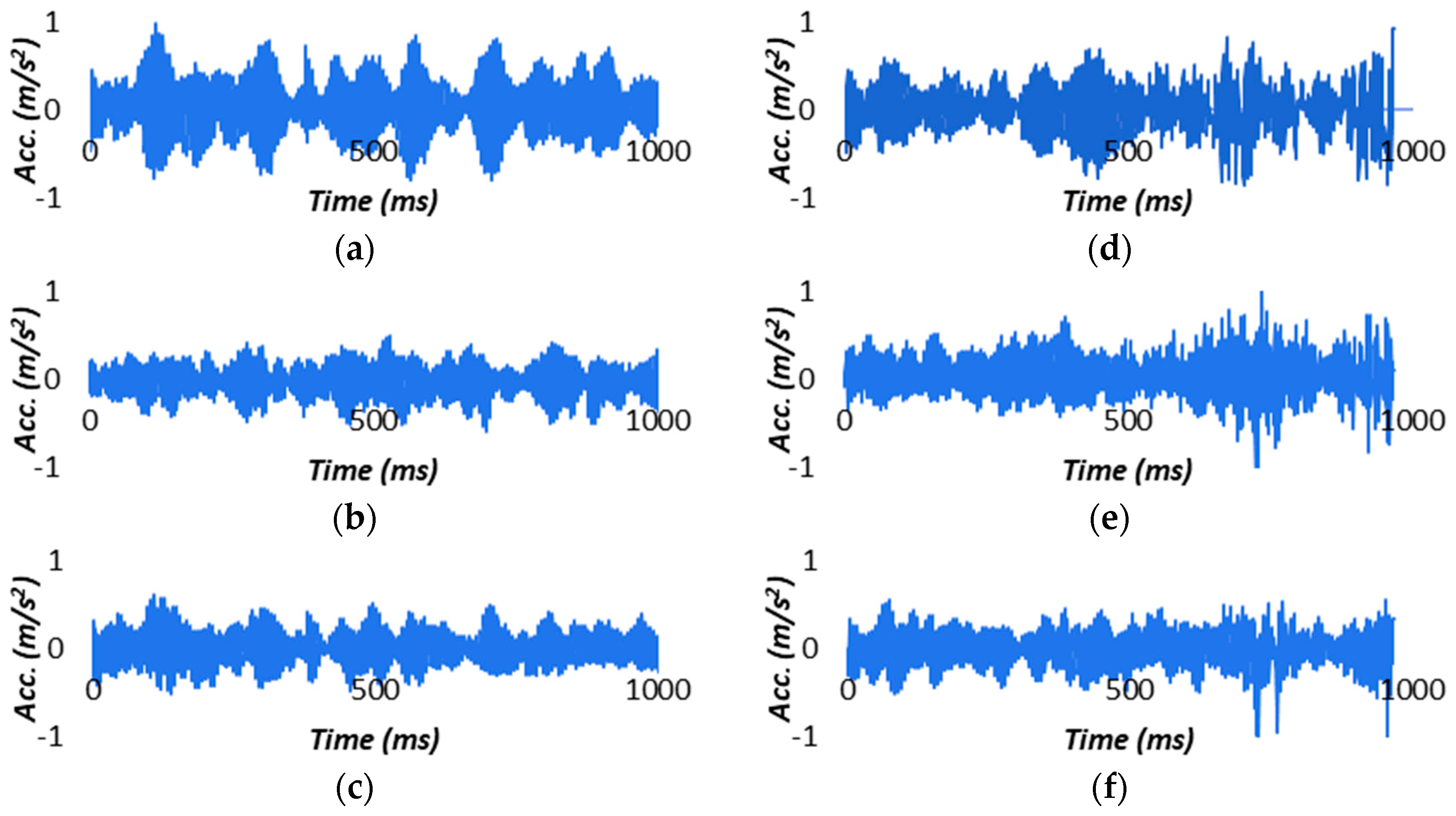
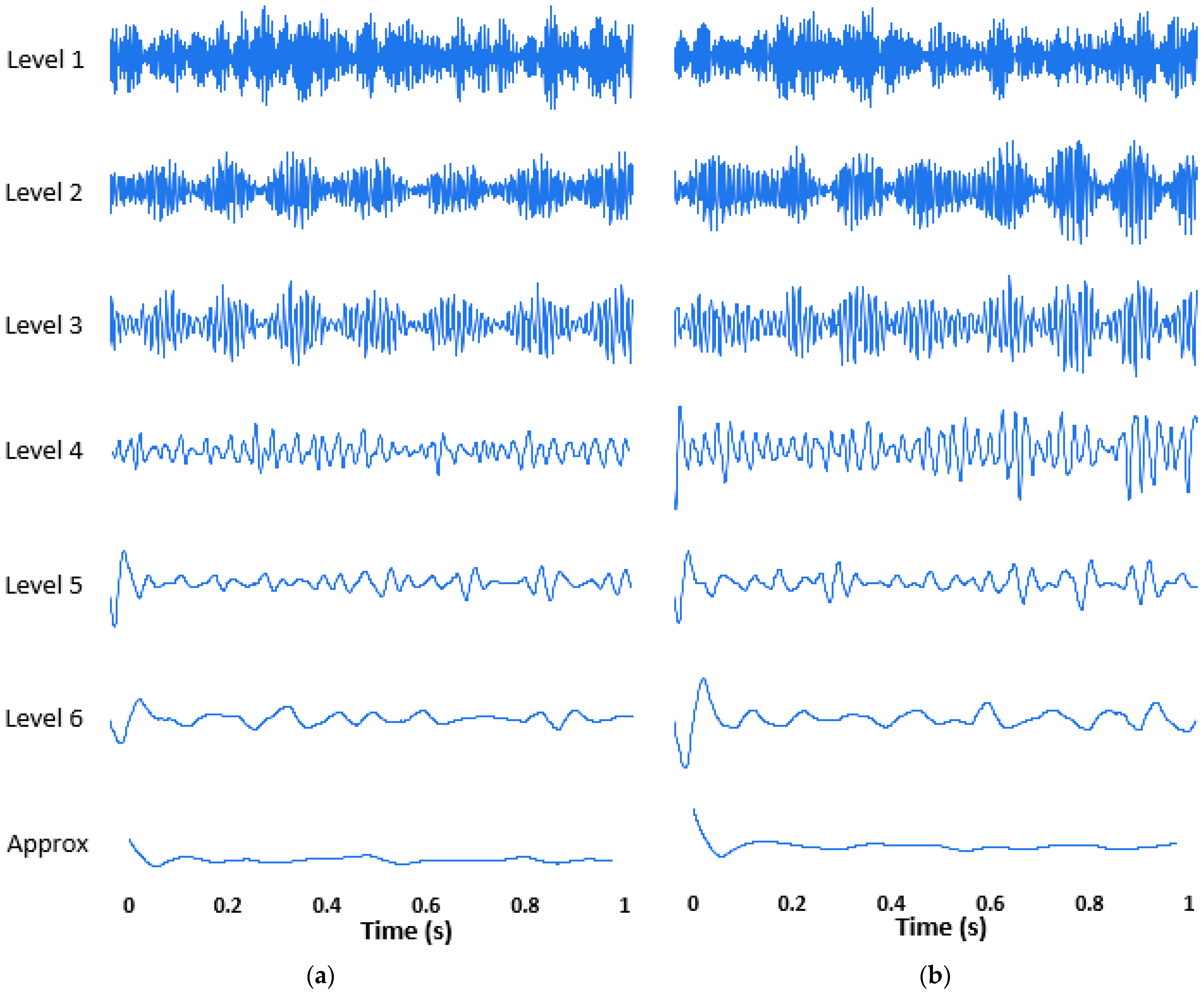
4.5. Signal Analysis
4.6. Statistical Features and Important Feature Selection
4.6.1. ReliefF
4.6.2. χ2
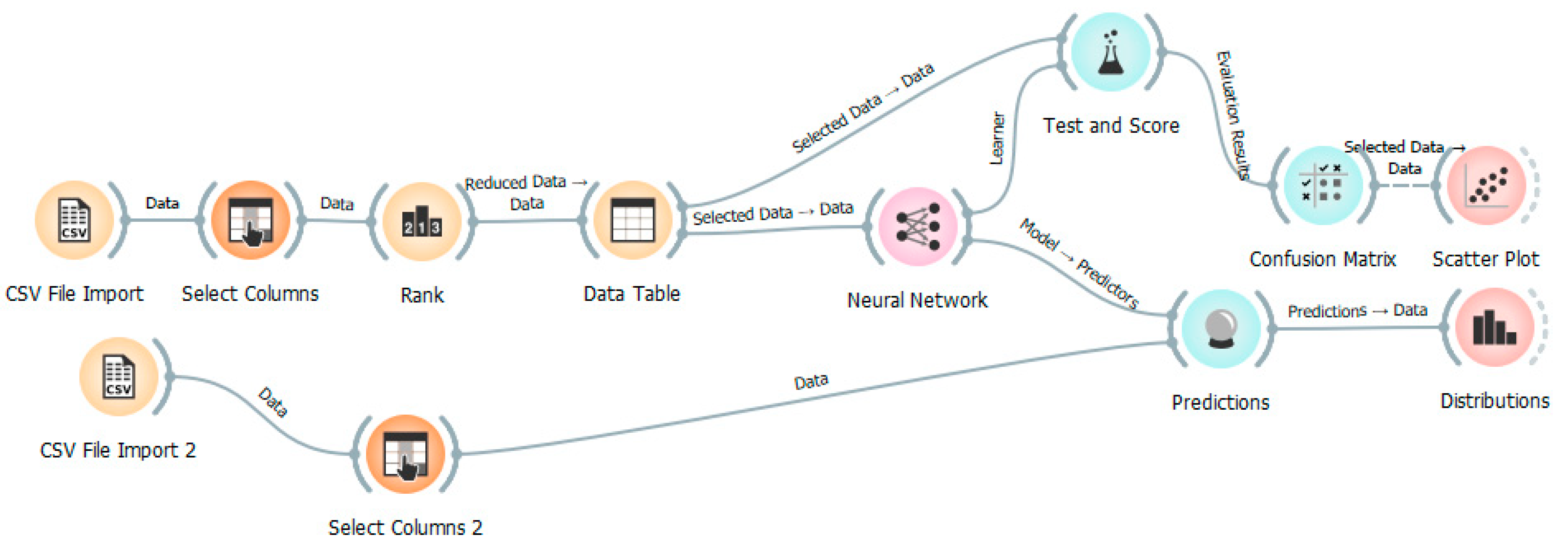
4.7. The Developed Orange Program for Deep Neural Network
5. Results and Discussion
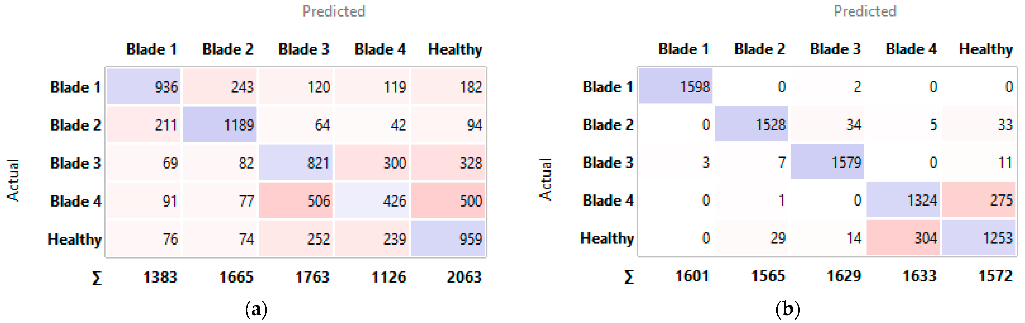
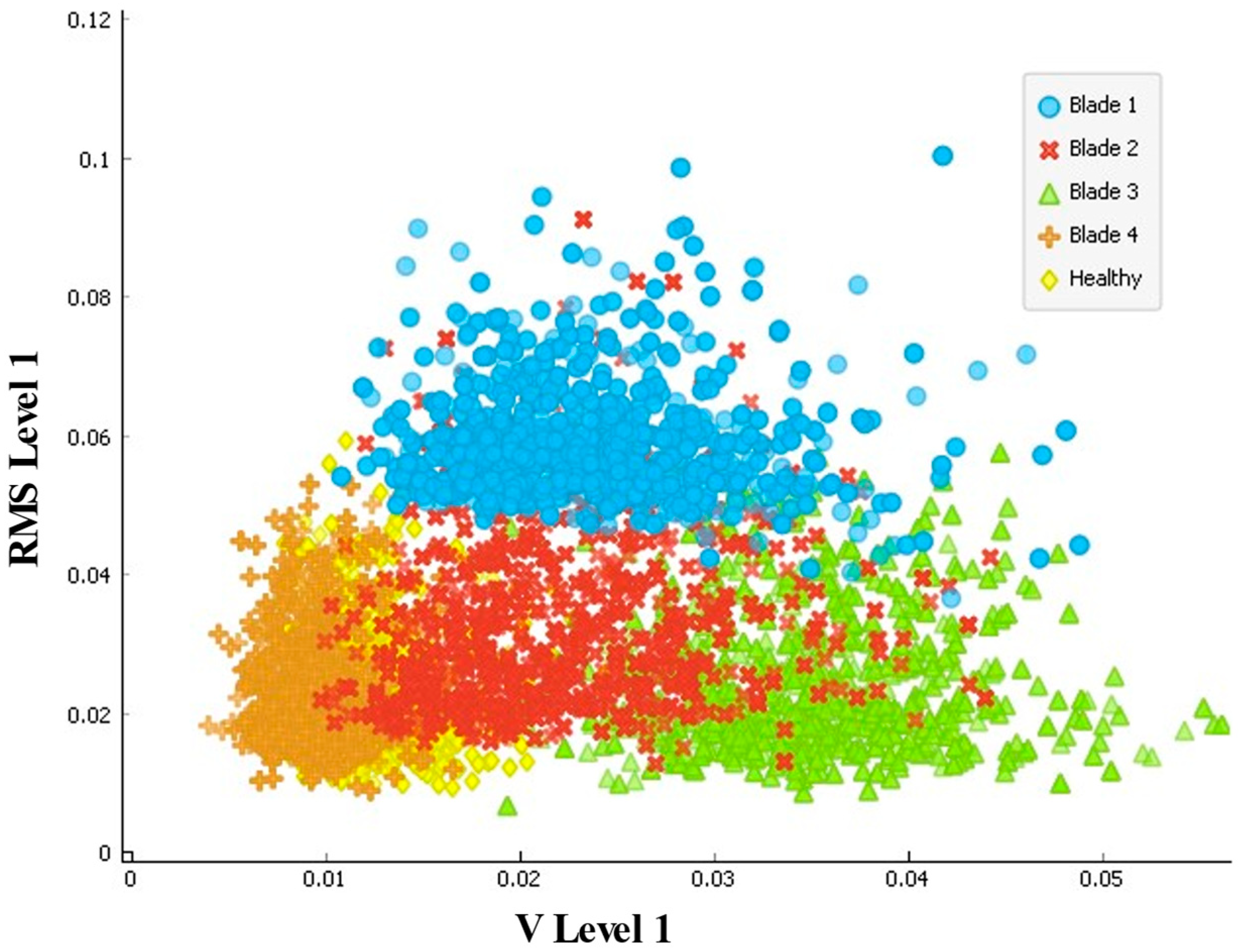
5.1. Test and Score
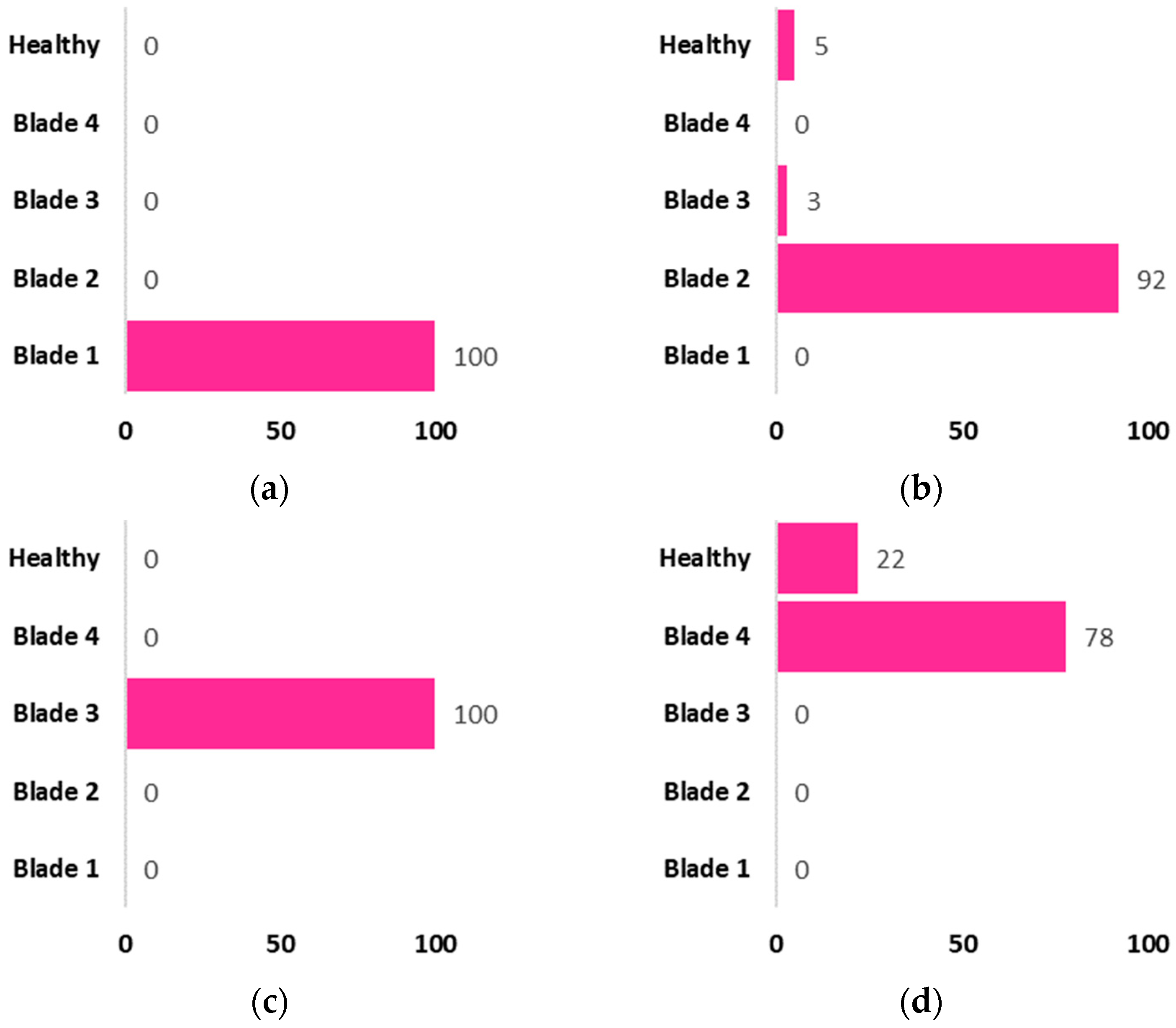
5.2. Model Validation
6. Conclusions
Author Contributions
Funding
Data Availability Statement
Acknowledgments
Conflicts of Interest
References
- Zieja, M.; Golda, P.; Zokowski, M.; Majewski, P. Vibroacoustic technique for the fault diagnosis in a gear transmission of a military helicopter. J. Vibroengineering 2017, 19, 1039–1049. [Google Scholar] [CrossRef]
- Sun, C.; Wang, Y.; Sun, G. A multi-criteria fusion feature selection algorithm for fault diagnosis of helicopter planetary gear train. Chin. J. Aeronaut. 2020, 33, 1549–1561. [Google Scholar] [CrossRef]
- Krichen, M.; Adoni, W.Y.H.; Mihoub, A.; Alzahrani, M.Y.; Nahhal, T. Security Challenges for Drone Communications: Possible Threats, Attacks and Countermeasures. In Proceedings of the 2022 2nd International Conference of Smart Systems and Emerging Technologies (SMARTTECH), Riyadh, Saudi Arabia, 9–11 May 2022; pp. 184–189. [Google Scholar] [CrossRef]
- Bunse, C.; Plotz, S. Security Analysis of Drone Communication Protocols. In Engineering Secure Software and Systems. ESSoS 2018; Lecture Notes in Computer Science; Payer, M., Rashid, A., Such, J., Eds.; Springer: Cham, Switzerland, 2018; Volume 10953. [Google Scholar] [CrossRef]
- Karbach, N.; Bobrowski, N.; Hoffmann, T. Observing volcanoes with drones: Studies of volcanic plume chemistry with ultralight sensor systems. Sci. Rep. 2022, 12, 17890. [Google Scholar] [CrossRef]
- Booysen, R.; Jackisch, R.; Lorenz, S.; Zimmermann, R.; Kirsch, M.; Nex, P.A.M.; Gloaguen, R. Detection of REEs with lightweight UAV-based hyperspectral imaging. Sci. Rep. 2020, 10, 17450. [Google Scholar] [CrossRef]
- Munawar, H.S.; Ullah, F.; Heravi, A.; Thaheem, M.J.; Maqsoom, A. Inspecting Buildings Using Drones and Computer Vision: A Machine Learning Approach to Detect Cracks and Damages. Drones 2021, 6, 5. [Google Scholar] [CrossRef]
- Brewer, M.J.; Clements, C.B. Meteorological Profiling in the Fire Environment Using UAS. Fire 2020, 3, 36. [Google Scholar] [CrossRef]
- Puchalski, R.; Giernacki, W. UAV Fault Detection Methods, State-of-the-Art. Drones 2022, 6, 330. [Google Scholar] [CrossRef]
- Medeiros, R.L.V.; Ramos, J.G.G.S.; Nascimento, T.P.; Filho, A.C.L.; Brito, A.V. A Novel Approach for Brushless DC Motors Characterization in Drones Based on Chaos. Drones 2018, 2, 14. [Google Scholar] [CrossRef]
- Yang, P.; Geng, H.; Wen, C.; Liu, P. An Intelligent Quadrotor Fault Diagnosis Method Based on Novel Deep Residual Shrinkage Network. Drones 2021, 5, 133. [Google Scholar] [CrossRef]
- Masalimov, K.; Muslimov, T.; Munasypov, R. Real-Time Monitoring of Parameters and Diagnostics of the Technical Condition of Small Unmanned Aerial Vehicle’s (UAV) Units Based on Deep BiGRU-CNN Models. Drones 2022, 6, 368. [Google Scholar] [CrossRef]
- Dai, W.; Liang, K.; Wang, B. State Monitoring Method for Tool Wear in Aerospace Manufacturing Processes Based on a Convolutional Neural Network (CNN). Aerospace 2021, 8, 335. [Google Scholar] [CrossRef]
- Xu, Z.; Chen, B.; Zhou, S.; Chang, W.; Ji, X.; Wei, C.; Hou, W. A Text-Driven Aircraft Fault Diagnosis Model Based on a Word2vec and Priori-Knowledge Convolutional Neural Network. Aerospace 2021, 8, 112. [Google Scholar] [CrossRef]
- Ai, S.; Song, J.; Cai, G.; Zhao, K. Active Fault-Tolerant Control for Quadrotor UAV against Sensor Fault Diagnosed by the Auto Sequential Random Forest. Aerospace 2022, 9, 518. [Google Scholar] [CrossRef]
- Wild, G.; Gavin, K.; Murray, J.; Silva, J.; Baxter, G. A Post-Accident Analysis of Civil Remotely-Piloted Aircraft System Accidents and Incidents. J. Aerosp. Technol. Manag. 2017, 9, 157–168. [Google Scholar] [CrossRef]
- Bhandari, S.; Jotautienė, E. Vibration Analysis of a Roller Bearing Condition Used in a Tangential Threshing Drum of a Combine Harvester for the Smooth and Continuous Performance of Agricultural Crop Harvesting. Agriculture 2022, 12, 1969. [Google Scholar] [CrossRef]
- Yao, Y.; Li, X.; Yang, Z.; Li, L.; Geng, D.; Huang, P.; Li, Y.; Song, Z. Vibration Characteristics of Corn Combine Harvester with the Time-Varying Mass System under Non-Stationary Random Vibration. Agriculture 2022, 12, 1963. [Google Scholar] [CrossRef]
- Oyarzun, J.; Aizpuru, I.; Baraia-Etxaburu, I. Time–Frequency Analysis of Experimental Measurements for the Determination of EMI Noise Generators in Power Converters. Electronics 2022, 11, 3898. [Google Scholar] [CrossRef]
- Sadeghi, S.M.; Mashadi, B.; Amirkhani, A.; Salari, A.H. Maximum tire/road friction coefficient prediction based on vehicle vertical accelerations using wavelet transform and neural network. J. Braz. Soc. Mech. Sci. Eng. 2022, 44, 324. [Google Scholar] [CrossRef]
- Leavey, C.M.; James, M.N.; Summerscales, J.; Sutton, R. An introduction to wavelet transforms: A tutorial approach. Insight-Non-Destr. Test. Cond. Monit. 2003, 45, 344–353. [Google Scholar] [CrossRef]
- Rajbhandari, S. Application of Wavelets and Artificial Neural Network for Indoor Optical Wireless Communication Systems. Ph.D. Thesis, School of Computing, Engineering and Information Sciences, University of Northumbria, Newcastle, UK, 2009. [Google Scholar]
- Giaouris, D.; Zahawi, B.; El-Murr, G.; Pickert, V. Application of Wavelet Transformation for the Identification of High Frequency Spurious Signals in Step Down DC—DC Converter Circuits Experiencing Intermittent Chaotic Patterns. In Proceedings of the 3rd IET International Conference on Power Electronics, Machines and Drives, Dublin, Ireland, 4–6 April 2006; pp. 394–397. [Google Scholar]
- Loutas, T.; Kostopoulos, V. Utilising the wavelet transform in condition-based maintenance: A review with applications. In Advances in Wavelet Theory and Their Applications in Engineering, Physics and Technology; Baleanu, D., Ed.; InTech: Rijeka, Croatia, 2012; pp. 273–312. ISBN 978-953-51-0494-0. [Google Scholar]
- Qu, J.; Zhang, Z.; Gong, T. A novel intelligent method for mechanical fault diagnosis based on dual-tree complex wave-let packet transform and multiple classifier fusion. Neurocomputing 2016, 171, 837–853. [Google Scholar] [CrossRef]
- Ong, P.; Tieh, T.H.C.; Lai, K.H.; Lee, W.K.; Ismon, M. Efficient gear fault feature selection based on moth-flame optimisation in discrete wavelet packet analysis domain. J. Braz. Soc. Mech. Sci. Eng. 2019, 41, 266. [Google Scholar] [CrossRef]
- Vivas, E.L.A.; Garcia-Gonzalez, A.; Figueroa, I.; Fuentes, R.Q. Discrete Wavelet Transform and ANFIS Classifier for Brain-Machine Interface based on EEG. In Proceedings of the 6th International Conference on Human System Interactions, Sopot, Poland, 6–8 June 2013; Paja, W.A., Wilamowski, B.M., Eds.; IEEE: New York, NY, USA, 2013; pp. 137–144. [Google Scholar]
- Misiti, M.; Misiti, Y.; Oppenheim, G.; Poggi, J.-M. Wavelet Toolbox For Use with MATLAB: MathWorks. 1997. Available online: http://cda.psych.uiuc.edu/matlab_pdf/wavelet_ug.pdf (accessed on 2 October 2022).
- Hariharan, M.; Fook, C.; Sindhu, R.; Ilias, B.; Yaacob, S. A comparative study of wavelet families for classification of wrist motions. Comput. Electr. Eng. 2012, 38, 1798–1807. [Google Scholar] [CrossRef]
- Gonçalves, M.A.; Gonçalves, A.S.; Franca, T.C.C.; Santana, M.S.; da Cunha, E.F.F.; Ramalho, T.C. Improved Protocol for the Selection of Structures from Molecular Dynamics of Organic Systems in Solution: The Value of Investigating Different Wavelet Families. J. Chem. Theory Comput. 2022, 18, 5810–5818. [Google Scholar] [CrossRef] [PubMed]
- Too, J.; Abdullah, A.R.; Saad, N.M.; Ali, N.M.; Musa, H. A Detail Study of Wavelet Families for EMG Pattern Recognition. Int. J. Electr. Comput. Eng. (IJECE) 2018, 8, 4221–4229. [Google Scholar] [CrossRef]
- Jaber, A.A.; Bicker, R. The optimum selection of wavelet transform parameters for the purpose of fault detection in an industrial robot. In Proceedings of the 2014 IEEE International Conference on Control System, Computing and Engineering (ICCSCE 2014), Penang, Malaysia, 28–30 November 2014; pp. 304–309. [Google Scholar]
- Katsavrias, C.; Papadimitriou, C.; Hillaris, A.; Balasis, G. Application of Wavelet Methods in the Investigation of Geospace Disturbances: A Review and an Evaluation of the Approach for Quantifying Wavelet Power. Atmosphere 2022, 13, 499. [Google Scholar] [CrossRef]
- Ma, L.; Zhang, S.; Cheng, L. A 2D Daubechies wavelet model on the vibration of rectangular plates containing strip indentations with a parabolic thickness profile. J. Sound Vib. 2018, 429, 130–146. [Google Scholar] [CrossRef]
- Su, B.; Xu, C.; Li, J. A Deep Neural Network Approach to Solving for Seal’s Type Partial Integro-Differential Equation. Mathematics 2022, 10, 1504. [Google Scholar] [CrossRef]
- Stanković, M.; Mirza, M.M.; Karabiyik, U. UAV Forensics: DJI Mini 2 Case Study. Drones 2021, 5, 49. [Google Scholar] [CrossRef]
- Casabianca, P.; Zhang, Y. Acoustic-Based UAV Detection Using Late Fusion of Deep Neural Networks. Drones 2021, 5, 54. [Google Scholar] [CrossRef]
- Ghazali, M.H.M.; Rahiman, W. An Investigation of the Reliability of Different Types of Sensors in the Real-Time Vibration-Based Anomaly Inspection in Drone. Sensors 2022, 22, 6015. [Google Scholar] [CrossRef]
- Jaber, A.A.; Bicker, R. A simulation of non-stationary signal analysis using wavelet transform based on LabVIEW and Matlab. In Proceedings of the UKSim-AMSS 8th European Modelling Symposium on Computer Modelling and Simulation, EMS 2014, Pisa, Italy, 21–23 October 2014; pp. 138–144. [Google Scholar] [CrossRef]
- Ewert, P.; Kowalski, C.T.; Orlowska-Kowalska, T. Low-Cost Monitoring and Diagnosis System for Rolling Bearing Faults of the Induction Motor Based on Neural Network Approach. Electronics 2020, 9, 1334. [Google Scholar] [CrossRef]
- Jawad, S.M.; Jaber, A.A. Bearings Health Monitoring Based on Frequency-Domain Vibration Signals Analysis. Eng. Technol. J. 2022, 41, 86–95. [Google Scholar] [CrossRef]
- Flaieh, E.H.; Hamdoon, F.O.; Jaber, A.A. Estimation the natural frequencies of a cracked shaft based on finite element modeling and artificial neural network. Int. J. Adv. Sci. Eng. Inf. Technol. 2020, 10, 1410–1416. [Google Scholar]
- Jaber, A.A.; Bicker, R. Industrial robot fault detection based on statistical control chart. Am. J. Eng. Appl. Sci. 2016, 9, 251–263. [Google Scholar] [CrossRef]
- Jaber, A.A.; Bicker, R. Development of a Condition Monitoring Algorithm for Industrial Robots based on Artificial Intelligence and Signal Processing Techniques. Int. J. Electr. Comput. Eng. (IJECE) 2018, 8, 996–1009. [Google Scholar] [CrossRef]
- Dhomad, T.A.; Jaber, A. Bearing fault diagnosis using motor current signature analysis and the artificial neural network. Int. J. Adv. Scince Eng. Inf. Technol. 2020, 10, 70–79. [Google Scholar] [CrossRef]
- Mohammed, J.S.; Abdulhady, J.A. Rolling bearing fault detection based on vibration signal analysis and cumulative sum control chart. FME Trans. 2021, 49, 684–695. [Google Scholar] [CrossRef]
- Altinors, A.; Yol, F.; Yaman, O. A sound based method for fault detection with statistical feature extraction in UAV motors. Appl. Acoust. 2021, 183, 108325. [Google Scholar] [CrossRef]
- Ma, L.; Fu, T.; Blaschke, T.; Li, M.; Tiede, D.; Zhou, Z.; Ma, X.; Chen, D. Evaluation of Feature Selection Methods for Object-Based Land Cover Mapping of Unmanned Aerial Vehicle Imagery Using Random Forest and Support Vector Machine Classifiers. ISPRS Int. J. Geo-Inf. 2017, 6, 51. [Google Scholar] [CrossRef]
- Sarra, R.R.; Dinar, A.M.; Mohammed, M.A.; Abdulkareem, K.H. Enhanced Heart Disease Prediction Based on Machine Learning and χ2 Statistical Optimal Feature Selection Model. Designs 2022, 6, 87. [Google Scholar] [CrossRef]
- Demsar, J.; Zupan, B. Orange: Data mining fruitful and fun-A historical perspective. Informatica 2013, 37, 55–60. [Google Scholar]
- Glowacz, A. Thermographic Fault Diagnosis of Shaft of BLDC Motor. Sensors 2022, 22, 8537. [Google Scholar] [CrossRef] [PubMed]
- Al-Haddad, S.A.; Al-Ani, F.H.; Fattah, M.Y. Effect of Using Plastic Waste Bottles on Soil Response above Buried Pipes under Static Loads. Appl. Sci. 2022, 12, 12304. [Google Scholar] [CrossRef]


| Ref. | Utilized Machine/Deep Learning and Signal Processing Approach | UAV Type |
|---|---|---|
| [10] | Signal Analysis based on Chaos using Density of Maxima (SAC-DM) and Fast Fourier Transform (FFT) | Brushless Direct Current (BLDC) motors’ behavior in a drone |
| [11] | Novel Deep Residual Shrinkage Network with a wide convolutional layer (1D-WIDRSN) | Quadrotor propellers with minor damage |
| [12] | Convolutional Neural Network | Carbon Z T-28 fixed-wing-type UAV fault simulators |
| [13] | Tool Wear in Aerospace Manufacturing Processes | |
| [14] | Real aircraft fault text data set | |
| [15] | Auto Sequential Random Forest | Quadrotor sensor fault |
| No. | Specification | Information |
|---|---|---|
| 1 | Dimension | 21 × 16 × 10 mm |
| 2 | Weight | 2 g |
| 3 | Operating voltage | 5 V |
| 4 | Operating current | 400 µA |
| 5 | Sensitivity | 300 mV/g |
| 6 | Bandwidth | 0.5–1600 Hz (x- and y-axes) and 0.5–550 Hz (z-axes) |
| 7 | Full-scale range | +/− 3 g |
| Case | Hovering Speed (RPM) | Hovering Speed (Hz) | Height From Ground (m) | Location of Damaged Blade |
|---|---|---|---|---|
| Healthy | 10,000 | 168 | 1.2 | - |
| Blade 1 Damaged | Bottom Right | |||
| Blade 2 Damaged | Top Right | |||
| Blade 3 Damaged | Top Left | |||
| Blade 4 Damaged | Bottom Left |
| Levels | 1 | 2 | 3 | 4 | 5 | 6 | Approx |
|---|---|---|---|---|---|---|---|
| Frequency Range (Hz) | 1024–512 | 512–256 | 256–128 | 128–64 | 64–32 | 32–16 | 16–0 |
| Evaluation Results | Train time (s) | Test time (s) | Area under Curve (AUC) | Classification Accuracy (CA) | Precision | Recall | Specificity |
|---|---|---|---|---|---|---|---|
| Value | 25.602 | 0.064 | 0.831 | 0.541 | 0.54 | 0.541 | 0.885 |
| Evaluation Results | Train time (s) | Test time (s) | Area under Curve (AUC) | Classification Accuracy (CA) | Precision | Recall | Specificity |
|---|---|---|---|---|---|---|---|
| Value | 25.093 | 0.057 | 0.987 | 0.91 | 0.91 | 0.91 | 0.978 |
Disclaimer/Publisher’s Note: The statements, opinions and data contained in all publications are solely those of the individual author(s) and contributor(s) and not of MDPI and/or the editor(s). MDPI and/or the editor(s) disclaim responsibility for any injury to people or property resulting from any ideas, methods, instructions or products referred to in the content. |
© 2023 by the authors. Licensee MDPI, Basel, Switzerland. This article is an open access article distributed under the terms and conditions of the Creative Commons Attribution (CC BY) license (https://creativecommons.org/licenses/by/4.0/).
Share and Cite
Al-Haddad, L.A.; Jaber, A.A. An Intelligent Fault Diagnosis Approach for Multirotor UAVs Based on Deep Neural Network of Multi-Resolution Transform Features. Drones 2023, 7, 82. https://doi.org/10.3390/drones7020082
Al-Haddad LA, Jaber AA. An Intelligent Fault Diagnosis Approach for Multirotor UAVs Based on Deep Neural Network of Multi-Resolution Transform Features. Drones. 2023; 7(2):82. https://doi.org/10.3390/drones7020082
Chicago/Turabian StyleAl-Haddad, Luttfi A., and Alaa Abdulhady Jaber. 2023. "An Intelligent Fault Diagnosis Approach for Multirotor UAVs Based on Deep Neural Network of Multi-Resolution Transform Features" Drones 7, no. 2: 82. https://doi.org/10.3390/drones7020082
APA StyleAl-Haddad, L. A., & Jaber, A. A. (2023). An Intelligent Fault Diagnosis Approach for Multirotor UAVs Based on Deep Neural Network of Multi-Resolution Transform Features. Drones, 7(2), 82. https://doi.org/10.3390/drones7020082