Quality-Aware Autonomous Navigation with Dynamic Path Cost for Vision-Based Mapping toward Drone Landing

Abstract

This article presents a novel autonomous navigation approach that is capable of increasing map exploration and accuracy while minimizing the distance traveled for autonomous drone landings. For terrain mapping, a probabilistic sparse elevation map is proposed to represent measurement accuracy and enable the increasing of map quality by continuously applying new measurements with Bayes inference. For exploration, the Quality-Aware Best View (QABV) planner is proposed for autonomous navigation with a dual focus: map exploration and quality. Generated paths allow for visiting viewpoints that provide new measurements for exploring the proposed map and increasing its quality. To reduce the distance traveled, we handle the path-cost information in the framework of control theory to dynamically adjust the path cost of visiting a viewpoint. The proposed methods handle the QABV planner as a system to be controlled and regulate the information contribution of the generated paths. As a result, the path cost is increased to reduce the distance traveled or decreased to escape from a low-information area and avoid getting stuck. The usefulness of the proposed mapping and exploration approach is evaluated in detailed simulation studies including a real-world scenario for a packet delivery drone.

1. Introduction

The academic research on drones is increasing as drone applications have been successfully used in search and rescue missions [1,2], warehouse management [3,4], surveillance and inspection [5,6], agriculture [7], and package delivery [8]. Although most drone autopilots have autonomous take-off and cruise functions [9,10], landing in an unknown environment is still one of the challenges to be tackled. To accomplish a safe landing, the drone must be aware of the area underneath to pick a safe landing area autonomously. In this context, large unmanned aerial vehicles use lidar-based active scanners to generate elevation maps [11,12], yet the usage of these scanners increases not only the weight but also its energy consumption. Alternatively, drones are equipped with camera systems that are lightweight and energy efficient. In developing a camera-based method for autonomous landing, the main challenges are (1) terrain mapping and (2) exploration.

For terrain mapping, a single-camera setup can be used for distance measurements of the terrain. In one of the earliest works [13], a method based on the recursive multi-frame planar parallax algorithm [14] is presented to map the environment via a single camera. In [15], a dense motion stereo algorithm processing a single camera is presented to concurrently assess feasible rooftop landing sites for a drone. In [16], a drone equipped with a single camera explores a previously unknown environment and generates a 3D point cloud map with a monocular visual simultaneous localization and mapping system (SLAM). Then, a grid map is generated from the point cloud data and appropriate landing zones are selected. In [17], fast semi-direct monocular visual odometry (SVO) [18] with a single camera is used for generating a sparse elevation map with Bayes inference to select a safe landing area away from obstacles. SVO has the highest computational efficiency among monocular state estimation and mapping techniques according to [19]. On the other hand, a stereo-camera setup is useful for depth measurements based on [20,21,22]. Compared to a single camera, a stereo camera (compromising a depth sensor) provides more accurate measurements, but they are heavier and more expensive than a single camera. Additionally, the resulting measurement error is a challenge. For instance, in [23], a stereo-camera system is used for the depth map generation of catastrophe-struck environments. In the depth map, measurements from higher altitudes have higher costs due to lower accuracy, and landing area selection is performed by considering the cost.

For exploration, there are many methods in the literature for path planning. In [13], a box-search method as a global plan combined with a predictive controller acts as a local path planner with online sensor information. In [15], to improve the landing site assessment, a path planner calculates optimal polynomial trajectories while ensuring the requirement for providing visual monitoring of a point of interest. In [24], the use of SVO is extended to a perception-aware receding horizon approach for drones to solve the active SLAM [25] problem and reach a target location safely and accurately. They generate arc-shaped candidate trajectories with [26] by using the information from SVO, then they select the best trajectory that maximizes the following metrics: collision probability, perception quality, and distance to the target location. To calculate the perception quality of each candidate trajectory, position samples are taken from each trajectory using a constant time interval. Then for each sample, the position estimation error is calculated by using the visible landmarks from SVO. The intuition is that more visible landmarks result in less position estimation error and accurate pose estimation along the trajectory can help better triangulate new landmarks, which is beneficial for the pose estimation afterward. In [20], the receding horizon “Next-Best-View” (NBV) planner is employed. The NBV planner makes use of rapidly-exploring random tree (RRT) [27] and suggests a receding horizon planning strategy. In every planning iteration, an RRT is generated and the best branch of the tree (i.e., a sequence of waypoints) is determined for map exploration. The intuition is that when a drone visits a waypoint in an RRT branch that provides a better viewpoint for map exploration, the exploration will be faster. The NBV planner selects the best branch with this intuition, but only the first step is executed as is in the receding horizon fashion. This process continues until the environment is explored except for residual locations such as occluded places and narrow pockets between objects. To improve the NBV planner regarding global map exploration, Schmit et al. [21] proposed using RRT* [28]; it obtains global exploration by continuously expanding a single trajectory tree, allowing the algorithm to maximize a single objective function. This enables the method to reason about the global utility of a path and refine trajectories to maximize their value. For the same purpose, Selin et al. [22] suggest using frontier exploration planning [29] as a global planner while using the NBV planner as a local planner.

In this study, we propose a novel autonomous navigation approach by considering map exploration and accuracy while minimizing the distance traveled for autonomous drone landings. The proposed overall approach is illustrated in Figure 1.

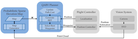
Figure 1. Probabilistic sparse elevation map generation and the QABV planner, marked in blue, are the main components of the proposed autonomous navigation approach for map exploration and accuracy toward drone landing. The flight controller and the vision system are used by the proposed approach during the map generation process.

For terrain mapping, we propose a “Probabilistic Sparse Elevation Map” to represent the area underneath a drone. As illustrated in Figure 1, the SVO approach takes image frames from a down-looking single camera attached to the drone, estimates the drone position, and generates point cloud data where each point is represented with a normal distribution. To generate the proposed map, we use point cloud data as height measurements and apply new measurements continuously with Bayes inference to increase the accuracy of the measurements. During this process, a path planner is also required to process map information and guide the drone to take the necessary measurements for map exploration and quality. When the map generation is completed, the final map can be used to identify safe landing areas for the drone.

For exploration, we propose the “Quality-Aware Best View (QABV) planner” to increase not only the accuracy of the map but also to decrease the traveled distance. To accomplish such a goal, we develop a novel information gain and dynamic path cost that allows the QABV planner to generate local waypoints considering map accuracy and exploration with traveled distance. In every planning iteration of QABV, an RRT with root node drone position is built and the best branch of the RRT is determined according to the information gain, which comprises the sum of the information contribution of each visible map cell for the subject branch. The intuition is that the more information we obtain from the visible area when we follow the RRT branch, the higher the map quality and exploration will increase. In this context, we calculate the information contribution of a visible map cell using its variance from the proposed probabilistic sparse elevation map information if it is updated before. If it is not, then we estimate its information contribution by calculating the height deviation of the visible area. After determining the best branch, the first node of the branch is sent to the position controller as the best waypoint. Through the proposed dynamic path cost approach, the QABV is capable of increasing the map exploration and accuracy while not increasing the traveled distance, thus ensuring traveling efficiency. We proposed using the node count between the subject node and the root node as the path cost and handling the dynamic path cost problem within the framework of control theory. We developed four novel approaches to increase efficiency by handling the QABV planner as the system to be controlled in order to regulate the information contribution of the generated paths. As a result, the path cost is increased to reduce the distance traveled or decreased to escape from a low-information area and avoid getting stuck.

The main contributions and outcomes of the study are summarized as follows:

• A probabilistic sparse elevation map generation algorithm with Bayes inference using SVO point cloud data and a down-looking single-camera setup. The generated map enables the representation of the sensor measurement accuracy to increase map quality by cooperating with the planner.
• A novel QABV planner for autonomous navigation with a dual focus: map exploration and quality. Generated paths via the novel information gain allow for visiting viewpoints that provide new measurements that increase the performance of the probabilistic sparse elevation map concerning exploration and accuracy.
• A novel dynamic path cost representation for the QABV planner to reduce the distance traveled and escape from a low-information area. To dynamically adjust the path cost, we propose four control methods: method 1 offers a simple approach with an on–off controller while method 2 employs a PD controller to adjust the path cost, and method 3 switches its control action depending on the reference while method 4 generates its reference depending on the map information.
• To show the performance improvements of the proposed approach, we present comparative simulation results. We demonstrate that the developed QABV planners have significantly better performances compared to the NBV planner regarding measurement accuracy and distance traveled.
• To verify the performance, we also solve the safe landing problem of a delivery drone within a realistic simulation environment. The results verify the usefulness of the proposed mapping and exploration approach.

2. Probabilistic Sparse Elevation Map Generation with SVO Point Cloud Data

In this section, we present the generation of the proposed probabilistic sparse elevation map that enhances the SVO point cloud data through the deployment of Bayes inference. The generated map provides measurement accuracy alongside the height of the terrain, which is processed by the proposed QABV planner to increase the accuracy of a location through Bayes inference.

2.1. SVO Point Cloud Data Generation

SVO estimates the position of image features (e.g., edges, points, and lines), and the estimation accuracy is defined by its uncertainty model [17,30]. In a single down-looking camera scenario, as illustrated in Figure 2, SVO first finds the transition vector $\mathit{d}=\overrightarrow{{\mathit{C}}_{\mathbf{0}}{\mathit{C}}_{\mathbf{1}}}$ between camera positions, and then solves the feature correspondence problem between consecutive images $I_0$ and $I_1$. Once an image feature correspondence is found between two images as $\mathit{u}$ and ${\mathit{u}}^{\prime }$, the position of the feature $\mathit{p}$ is estimated with triangulation.

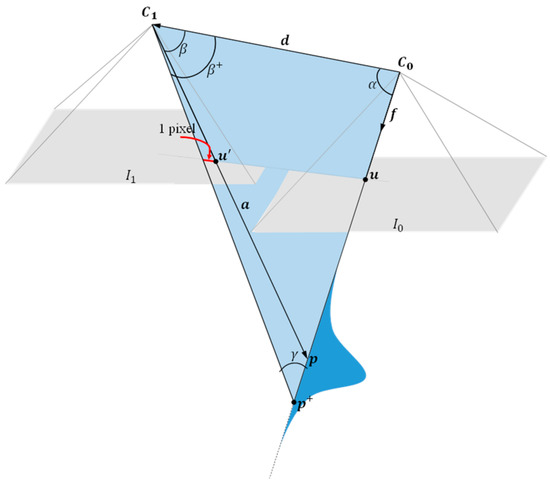
Figure 2. Illustration of the position estimation approach with SVO through a single down-looking camera.

As shown in Figure 2, the accuracy of this estimation is modeled as $N\left(\mathit{\mu },{\sigma }^2\right)$ and ${\sigma }^2$ corresponds to the assumption that a pixel error has occurred along the epipolar line passing through $\mathit{u}$ and ${\mathit{u}}^{\prime }$ while solving the feature correspondence problem. In this case, the position of the feature $\mathit{p}$ occurs in ${\mathit{p}}^{+}$, and the distance between them determines ${\sigma }^2$. To provide a clear explanation of the calculation of ${\sigma }^2$ and ${\mathit{p}}^{+}$, let us define the unit vector $\mathit{f}=\frac{\overrightarrow{{\mathit{C}}_{\mathbf{0}}\mathit{p}}}{\overrightarrow{\Vert {\mathit{C}}_{\mathbf{0}}\mathit{p}\Vert }}$ and the vector $\mathit{a}=\overrightarrow{{\mathit{C}}_{\mathbf{1}}\mathit{p}}$ as follows:

$$\mathit{a}=\overrightarrow{{\mathit{C}}_{\mathbf{0}}\mathit{p}}-\mathit{d}.$$

(1)

By using vector algebra, we can define the angle $\mathsf{\alpha }$ between vectors $\mathit{f}$ and $\mathit{d}$ as:

$$\mathsf{\alpha }=\arccos \left(\frac{\mathit{f}·\mathit{d}}{\Vert \mathit{d}\Vert }\right)$$

(2)

and the angle $\mathsf{\beta }$ between vectors $\mathit{a}$ and $-\mathit{d}$ as follows:

$$\mathsf{\beta }=\arccos \left(-\frac{\mathit{a}·\mathit{d}}{\Vert \mathit{a}\Vert \Vert \mathit{d}\Vert }\right).$$

(3)

We can add the angle spanning a pixel to $\mathsf{\beta }$ to find ${\mathsf{\beta }}^{+}$ when $\zeta$ is the camera focal length as [30]:

$${\mathsf{\beta }}^{+}=\mathsf{\beta }+2{\tan }^{-1}\left(\frac{1}{2\zeta }\right).$$

(4)

Now, we can calculate the angle $\gamma$ illustrated in Figure 2 by using the triangle sum theorem as follows:

$$\gamma =\mathsf{\pi }-\mathsf{\alpha }-{\mathsf{\beta }}^{+}.$$

(5)

Then, the norm of $\overrightarrow{{\mathit{C}}_{\mathbf{0}}{\mathit{p}}^{+}}$ is defined via the law of sines:

$$\overrightarrow{\Vert {\mathit{C}}_{\mathbf{0}}{\mathit{p}}^{+}\Vert }=\Vert \mathit{d}\Vert \frac{sin{\mathsf{\beta }}^{+}}{\sin \gamma }.$$

(6)

Therefore, when there is a pixel error while solving the feature correspondence problem for $\mathit{p}$, the measurement uncertainty is [30]:

$${\sigma }^2={(\Vert \overrightarrow{{\mathit{C}}_{\mathbf{0}}{\mathit{p}}^{+}}\Vert -\Vert {\overrightarrow{{\mathit{C}}_{\mathbf{0}}\mathit{p}}}^{}\Vert )}^2.$$

(7)

2.2. Probabilistic Sparse Elevation Map Generation via Bayesian Inference

The proposed probabilistic sparse elevation map $\mathit{M}$ uses a 2D matrix to represent the area underneath the drone on a grid, with each element ($Cell\left(i,j\right)$) corresponding to a point on the grid and representing a height measurement. During the generation of the map, each point $\mathit{p}=\left[x,y,z\right]$ in the SVO point cloud, along with its corresponding uncertainty (${\sigma }^2$), is continuously processed using Bayesian inference to update the corresponding $Cell\left(i,j\right)$ in $\mathit{M}$. This process takes place as the drone flies over an area, as shown in Figure 3.

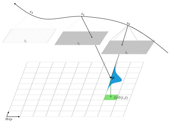
Figure 3. Update of a map cell with a point from SVO point cloud. By analyzing consecutive images from a single down-looking camera, the SVO algorithm does a probabilistic measurement of a point $\mathit{p}=\left[x,y,z\right]$ represented as normal distribution $N\left(\mathit{\mu },{\sigma }^2\right)$. $Cell\left(i,j\right)$ is updated with $z$ and ${\sigma }^2$ after matching $\mathit{p}$ in the 2D $xy$ map $\mathit{M}$.

In Algorithm 1, the pseudo-code of the proposed map generation approach is presented. Here, each $Cell\left(i,j\right)$ of $\mathit{M}$ is initialized with an unmapped cell defined as follows:

$$UnmappedCell=\left\{Cell\left(i,j\right)\right|Cell\left(i,j\right)\in \mathit{M},andCell\left(i,j\right)=\varnothing \}.$$

(8)

Then, $GetPointClou\mathit{d}()$ parses the SVO data stream and extracts every $\mathit{p}=\left[x,y,z\right]$ together with its ${\sigma }^2$. For each $\mathit{p}$ in the point cloud, $GetRelatedCell\left(\mathit{M},\mathit{p}\right)$ retrieves the corresponding $Cell\left(i,j\right)$ according to the $x$ and $y$ positions of $\mathit{p}$ so that it can be updated. In updating $Cell\left(i,j\right)$:

• If it is an unmapped cell, then its height $z$ and variance ${\sigma }^2$ are updated via $\mathit{p}$.
• If it is updated before but has more than $\pm 1\mathrm{cm}$ height error (i.e., a threshold value), then it is defined as an inaccurate cell as follows:

$$InaccurateCell=\left\{Cell\left(i,j\right)\right|Cell\left(i,j\right)\in \mathit{M},and{\sigma }^2>0.00001\},$$

(9)

and updated with $N\left(\mathit{\mu },{\sigma }^2\right)$ by applying the Bayes inference that is defined as follows:

$$N_{new}\left({\mathit{\mu }}_n,{\sigma }_n^2\right)=N_{old}\left({\mathit{\mu }}_o,{\sigma }_o^2\right)N\left(\mathit{\mu },{\sigma }^2\right).$$

(10)

where $\mathit{\mu }$ is the height measurement $z$, and $N_{old}\left({\mathit{\mu }}_o,{\sigma }_o^2\right)$ is the prior distribution. The resulting ${\mathit{\mu }}_n$ and ${\sigma }_n^2$ are defined using Bayes inference as:

$${\mathit{\mu }}_n=\frac{{\sigma }_o^2}{{\sigma }_o^2+{\sigma }_{}^2}\mathit{\mu }+\frac{{\sigma }_{}^2}{{\sigma }_o^2+{\sigma }_{}^2}{\mathit{\mu }}_o$$

(11)

$${\sigma }_n^2=\frac{1}{\frac{1}{{\sigma }_o^2}+\frac{1}{{\sigma }^2}}.$$

(12)

The generation of $\mathit{M}$ continues by parsing the SVO point cloud and updating the corresponding $Cell\left(i,j\right)$ until one of the selected stop criteria, such as map exploration or map accuracy, is satisfied. The map exploration measure is defined as follows:

$$M_{Ma\mathit{p}}(\%)=\frac{n\left(\mathit{M}\right)-n\left(UnmappedCell\right)}{n\left(\mathit{M}\right)}x100.$$

(13)

Map accuracy, on the other hand, is a more challenging measure since inaccurate cells include all unmapped cells and is defined as:

$$M_{Acc}(\%)=\frac{n\left(\mathit{M}\right)-n\left(InaccurateCell\right)}{n\left(\mathit{M}\right)}x100.$$

(14)

The computational complexity of Algorithm 1 cannot be calculated since satisfying the stop criterion is dependent on external processes such as the QABV planner and SVO; however, for a single run inside the while loop, the complexity of the $GetPointCloud()$ is $\mathcal{O}\left(siz{e}_{pc}\right)$ where $siz{e}_{pc}$ is the size of the point cloud data. The for loop runs for every point in the cloud, and inside the loop, every operation costs the same amount of time, so its complexity is $\mathcal{O}\left(siz{e}_{pc}\right)$. Lastly, the complexity of checking either of the stop criterion defined in (13) and (14) is $\mathcal{O}\left(siz{e}_{\mathit{M}}\right)$, where $siz{e}_{\mathit{M}}$ is the size of $\mathit{M}$. In this case, total complexity is $\mathcal{O}\left(2siz{e}_{pc}+siz{e}_{\mathit{M}}\right)$.

Algorithm 1. Sparse Elevation Map Generation via Bayes Inference

1:$\mathit{M}\leftarrow$ Initialize with unmapped cells 2: while the stop criterion is not satisfied ($M_{Map}$ or $M_{Acc}$) 3: $pc\leftarrow GetPointClou\mathit{d}()$ 4:     for each $\mathit{p}$ in $pc$ do 5:         $Cell\left(i,j\right)\leftarrow GetRelatedCell\left(\mathit{M},\mathit{p}\right)$ 6:         if $Cell\left(i,j\right)$ is $Unmappe\mathit{d}Cell$ 7:             $Cell\left(i,j\right).height\leftarrow \mathit{p}.height$ 8:             $Cell\left(i,j\right).variance\leftarrow \mathit{p}.variance$ 9:         else if $Cell\left(i,j\right)$ is $InaccurateCell$ 10:             $Cell\left(i,j\right).height\leftarrow BayesInference\left(Cell\left(i,j\right).height,\mathit{p}.height\right)$ 11:             $Cell\left(i,j\right).variance\leftarrow BayesInference\left(Cell\left(i,j\right).variance,\mathit{p}.variance\right)$ 12:         end if 13:     end for 14: end while

Figure 4 is an example 3D illustration of the proposed probabilistic sparse elevation map constructed from $\mathit{M}$. Different than showing only height information such as in [17], our map keeps the variance information of the SVO point cloud and presents height information in a probabilistic way.

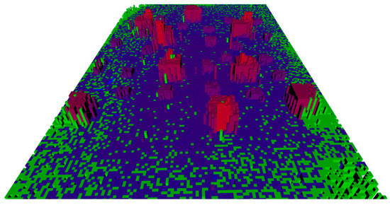
Figure 4. An example of constructed 3D sparse elevation map with SVO point cloud data. Here, the ground area is 12 m × 18.6 m and it consists of 10 cm × 10 cm map cells. Color codes indicate the status of the cells; green indicates inaccurate cells, and color tones between blue and red indicate cell height: blue for low, and red for high height. Void sections indicate unmapped cells.

3. Autonomous Navigation for Map Exploration and Accuracy

In this section, we present the proposed autonomous navigation method for map exploration and accuracy that is illustrated in Figure 1. Here, the developed QABV planner generates the best viewpoints for map exploration while considering measurement accuracy and distance traveled. The proposed QABV planner, similar to the NBV planner [20], generates a geometric tree with RRT [27] and selects the best branch of the tree (i.e., a series of waypoints that provides the best viewpoints) by analyzing the map M. The main differences between the QABV and NBV planners are:

• The QABV planner is capable of acquiring information and guiding the drone with a single down-looking camera unlike using a dual camera as in the NBV planner, as it uses the generated sparse probabilistic elevation map described in Section 2.
• Unlike the NBV planner which focuses only on map exploration, the proposed QABV planner has a dual focus on map exploration and quality thanks to a novel information gain function definition. The QABV analyzes the unmapped and inaccurate cells defined in (8) and (9) to generate the best waypoints such that new map cells are updated while the accuracy of previously updated cells is improved.
• The NBV planner has a global map coverage problem and gets stuck in large environments [21,22]. This increases the distance traveled or even causes failure in exploring all regions. On the other hand, the QABV planner uses a dynamic path cost to reduce the distance traveled.
• Especially in real-world applications, the path cost of the NBV planner becomes ineffective when the drone operates at a constant speed and the planner algorithm runs periodically. The QABV planner tackles this issue by processing the node numbers of the RRT branch as the path cost and adjusting its behavior dynamically while the map is being generated.

In the remaining part of this section, we first present a brief information NBV planner and describe its potentiation issues, then present all the details of the proposed QABV planner.

3.1. The NBV Planner: The Receding Horizon Next Best View Planner

As presented in Algorithm 2, the NBV planner employs a sampling-based receding horizon path planning paradigm for exploring a bounded 3D space $\mathit{V}\subset R^3$ via a drone equipped with a stereo camera [20]. Through the acquired information from depth images of the stereo camera, it generates an occupancy map $\mathcal{M}$, dividing $\mathit{V}$ into cubical volumes $\mathit{m}\in \mathcal{M}$ [31]. These cubical volumes can either be marked as free, occupied, or unmapped. The map $\mathcal{M}$ is used for both collision-free navigation through the known free space and for determining the exploration progress.

In [20], a collision-free vehicle position is $\mathit{\xi }={\left(x,y,z,\phi \right)}^T$, a path from ${\mathit{\xi }}_{k-1}$ to ${\mathit{\xi }}_k$ is denoted by $l_{k-1}^k$, and the cost of following this path is defined as:

$$c\left(l_{k-1}^k\right)=\sqrt{{\left(x_k-x_{k-1}\right)}^2+{\left(y_k-y_{k-1}\right)}^2+{\left(z_k-z_{k-1}\right)}^2}$$

(15)

In every planning iteration, starting from the current position of the vehicle ${\mathit{\xi }}_0$, a geometric tree $\mathbb{T}$ is incrementally built with RRT [27] by adding a new node $n$. The resulting $\mathbb{T}$ contains $N_{\mathbb{T}}$ nodes connected with collision-free and trackable paths, considering the dynamic and kinematic constraints of the drone.

NBV planner determines the best branch of $\mathbb{T}$ with a gain function, focusing on map exploration. For a given $\mathcal{M}$, the set of visible and unmapped cells from position $\mathit{\xi }$ is denoted as $Visible\left(\mathcal{M},\mathit{\xi }\right)$ [20]. Every cell in this set lies in the Field of View (FoV) of the camera and the direct line of sight does not cross other cells, so the cells are not occluded. In this case, the gain of a node $Gain\left(n\right)$ is the summation of unmapped cells that can be explored by the nodes along the branch. The gain of the node k is as follows [20]:

$$Gain\left(n_k\right)=Gain\left(n_{k-1}\right)+Visible\left(\mathcal{M},{\mathit{\xi }}_k\right)e^{-\lambda c\left(l_{k-1}^k\right)}$$

(16)

where $\lambda$ is the tuning factor for penalizing high path costs.

As presented in Algorithm 2, after every replanning of the NBV, the first segment of the branch to the best node $ExtractBestPathSegment\left(n_{best}\right)$ is returned and executed by the drone, where $n_{best}$ is the node with the highest gain. The remainder of the best branch is used to reinitialize $\mathbb{T}$ in the next run after re-evaluating its gain using the updated map $\mathcal{M}$ [20]. The creation of $\mathbb{T}$ is stopped at $N_{\mathbb{T}}=N_{max}$ in general, but if the best gain $g_{best}$ remains zero, tree construction is continued, until $g_{best}>0$. In the NBV algorithm, the map exploration problem is considered to be solved when $N_{\mathbb{T}}=N_{TOL}$ while $g_{best}$ remained zero. $N_{TOL}$ is a tolerance value that is significantly higher than $N_{max}$.

Algorithm 2. Receding Horizon Next Best View Planner [20]

1:${\mathit{\xi }}_0\leftarrow$ Current vehicle position 2: Initialize $\mathbb{T}$ with ${\mathit{\xi }}_0$ and, unless the first planner call, also previous best branch 3:$g_{best}\leftarrow 0$, set the best gain to zero 4:$n_{best}\leftarrow n_0$(${\mathit{\xi }}_{\mathbf{0}}$), set the best node to the root 5:$N_{\mathbb{T}}\leftarrow$ Number of initial nodes in $\mathbb{T}$ 6: while $N_{\mathbb{T}}<N_{max}$ or $g_{best}=0$ do 7:     Incrementally build $\mathbb{T}$ by adding $n_{new}\left({\mathit{\xi }}_{new}\right)$ 8:     $N_{\mathbb{T}}\leftarrow N_{\mathbb{T}}+1$ 9:     if $Gain\left(n_{new}\right)>g_{best}$ then 10:       $n_{best}\leftarrow n_{new}$ 11:       $g_{best}\leftarrow Gain\left(n_{new}\right)$ 12:     end if 13:     if $N_{\mathbb{T}}>N_{TOL}$ then 14:       Terminate exploration 15:     end if 16: end while 17:$l\leftarrow ExtractBestPathSegment\left(n_{best}\right)$ 18: Delete $\mathbb{T}$ 17: return $l$

The computational complexity of Algorithm 2 is dependent on the number of nodes in the tree $N_{\mathbb{T}}$, stereo camera range $d^{sensor}$, and a bounded 3D space to be explored $\mathit{V}$. The RRT creation complexity in a fixed environment is $\mathcal{O}\left(N_{\mathbb{T}}log\left(N_{\mathbb{T}}\right)\right)$, and the query of the best node is $\mathcal{O}\left(N_{\mathbb{T}}\right)$ [20]. A query complexity to map $\mathcal{M}$ is $\mathcal{O}\left(log\left(\mathit{V}/v^3\right)\right)$, where $v^3$ is a map element volume and collision check complexity is $\mathcal{O}\left(N_{\mathbb{T}}/v^{3}log\left(\mathit{V}/v^3\right)\right)$ for planning paths through known free space in $\mathcal{M}$ [20]. Additionally, the gains for every node in the RRT are computed. While considering a visible area by the stereo camera proportional to ${\mathit{V}}_{sensor}\propto {\left(d^{sensor}\right)}^3$, the number of queries to $\mathcal{M}$ approximates to ${\mathit{V}}_{sensor}/v^3$ for a node gain calculation. Additionally, the map elements on the ray $d^{sensor}/v$ are checked for visibility. So, the complexity of gain calculation for one node is $\mathcal{O}\left({\left(d^{sensor}/v\right)}^{4}log\left(\mathit{V}/v^3\right)\right)$ [20]. As a result, the total complexity of a single planning iteration is the sum of tree construction, collision-checking, and gain computation as follows [20]:

$$\mathcal{O}\left(N_{\mathbb{T}}log\left(N_{\mathbb{T}}\right)+N_{\mathbb{T}}/v^{3}log\left(\mathit{V}/v^3\right)+N_{\mathbb{T}}{\left(d^{sensor}/v\right)}^{4}log\left(\mathit{V}/v^3\right)\right).$$

(17)

The potential issues and improvement points of the NBV planner are as follows:

(P-i)

The gain function presented in (16) focuses only on map exploration without considering map quality; however, the measurement accuracy of the camera affects the quality of the map. By improving the $Visible\left(\mathcal{M},\mathit{\xi }\right)$ function, determining the exploration progress can be performed while improving the map quality.

(P-ii)

The path cost function in (15) uses the distance between adjacent nodes; when the algorithm runs periodically and drone speed is constant, then the distance between adjacent nodes is equal. Thus, the NBV planner cannot punish long-path costs. For a clear understanding, let us explain this issue via the scenario depicted in Figure 5. In this case, the path cost (15) is the same for the following paths:

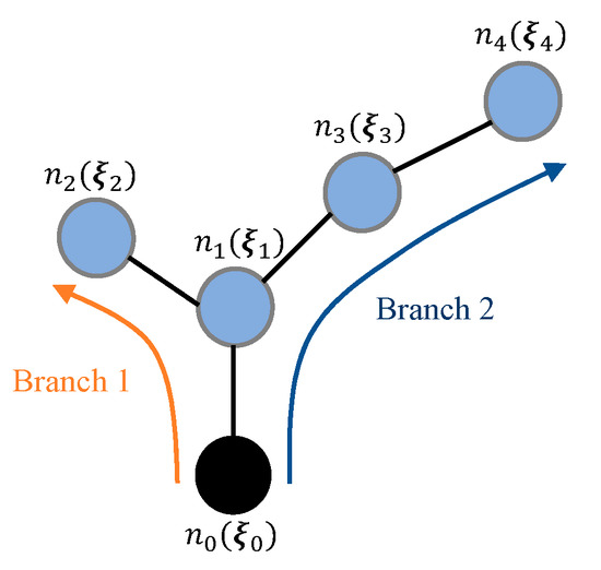Figure 5. Illustration of a geometric tree based on RRT.

$$c\left(l_1^2\right)=c\left(l_1^3\right)=c\left(l_3^4\right)$$

(18)

When visible unexplored map information at RRT Branch 1 is equal to the visible unexplored map information of both $n_3\left({\mathit{\xi }}_3\right)$ and $n_4({\mathit{\xi }}_4)$ in RRT Branch 2 as follows:

$$Visible\left(\mathcal{M},{\mathit{\xi }}_2\right)=Visible\left(\mathcal{M},{\mathit{\xi }}_3\right)+Visible\left(\mathcal{M},{\mathit{\xi }}_4\right),$$

(19)

then, according to (16), the gain of $n_2({\mathit{\xi }}_2)$ and $n_4({\mathit{\xi }}_4)$ are identical since (18) and (19) are equal. Thus, we can state that:

$$Visible\left(\mathcal{M},{\mathit{\xi }}_2\right)e^{-\lambda c\left(l_1^2\right)}=Visible\left(\mathcal{M},{\mathit{\xi }}_3\right)e^{-\lambda c\left(l_1^3\right)}+Visible\left(\mathcal{M},{\mathit{\xi }}_{new}\right)e^{-\lambda c\left(l_3^4\right)}$$

(20)

$$Gain\left(n_2\right)=Gain\left(n_4\right).$$

(21)

This shows that the NBV planner cannot decide in favor of Branch 1 despite having the same visible unexplored map information as Branch 2 at a shorter distance. Therefore, there is a need to improve the path cost function definition.

(P-iii)

As mentioned in [21,22], the NBV planner has a global map coverage problem and gets stuck in large environments. This can partly be handled by the careful tuning of the λ parameter in (16); however, this has to be completed for every environment and it typically requires several attempts. As a better approach, λ can be updated while the map is being explored rather than keeping it constant as is in the NBV planner.

3.2. The Proposed QABV Planner: Quality-Aware Best View Planner

The QABV planner presented in Algorithm 3 is a new local planner for guiding the drone to the best viewpoints with a dual focus, namely map exploration and quality. It increases the map quality during exploration, as it processes the probabilistic sparse elevation map $\mathit{M}$ presented in Section 2. The QABV planner employs a sampling-based receding horizon path planning paradigm such as the NBV planner as presented in Algorithm 3. In every planning iteration ($r$), $\mathbb{T}$ is generated with RRT, starting from ${\mathit{\xi }}_{\mathbf{0}}$, by incrementally adding new collision-free nodes (i.e., waypoints) until the number of nodes reaches $N_{\mathbb{T}}$.

Algorithm 3. Quality-Aware Best View Planner

1:${\mathit{\xi }}_0\leftarrow$ Current vehicle position 2: Initialize $\mathbb{T}$ with ${\mathit{\xi }}_{\mathbf{0}}$ in the first run, unless the previous best branch 3: Initialize ${\acute{g}}_{best}$ with −1 in the first run, unless the previous $g_{best}$ 4: Initialize $\mathsf{\Delta }{\mathit{g}}_{\mathit{b}\mathit{e}\mathit{s}\mathit{t}}$ as an empty vector in the first run 5: Initialize $\lambda$ with ${\lambda }_{init}$ in the first run 6: Set $\lambda$, update method in the first run: $\mathrm{method}\in \left\{1,2,3,4\right\}$ 7:$g_{best}\leftarrow 0$, set the best gain to zero 8:$n_{best}\leftarrow n_0$(${\mathit{\xi }}_{\mathbf{0}}$), set the best node to the root 9:$N_{\mathbb{T}}\leftarrow$ Number of initial nodes in $\mathbb{T}$ 10: switch $\mathrm{method}$ 11:     case 1: $\lambda \leftarrow Method1(\mathsf{\Delta }{\mathit{g}}_{\mathit{b}\mathit{e}\mathit{s}\mathit{t}},\lambda$) 12:     case 2: $\lambda \leftarrow Method2({\acute{g}}_{best},\mathsf{\Delta }{\mathit{g}}_{\mathit{b}\mathit{e}\mathit{s}\mathit{t}},\lambda$) 13:     case 3: $\lambda \leftarrow Method3({\acute{g}}_{best},\mathsf{\Delta }{\mathit{g}}_{\mathit{b}\mathit{e}\mathit{s}\mathit{t}},\lambda$) 14:     case 4: 15:       $M_{Acc}\leftarrow GetMapAccuracy\left(\mathit{M}\right)$ 16:       $\lambda \leftarrow Method4\left({\acute{g}}_{best},\mathsf{\Delta }{\mathit{g}}_{\mathit{b}\mathit{e}\mathit{s}\mathit{t}},\lambda ,M_{Acc}\right)$ 17: end switch 18: while $N_{\mathbb{T}}<N_{max}$ or $g_{best}=0$ do 19:     Incrementally build $\mathbb{T}$ by adding $n_{new}\left({\mathit{\xi }}_{new}\right)$ 20:     $N_{\mathbb{T}}$ ← $N_{\mathbb{T}}+1$ 21:     if $Gain\left(n_{new},\lambda \right)>g_{best}$ then 22:       $n_{best}\leftarrow n_{new}$ 23:       $g_{best}\leftarrow Gain\left(n_{new},\lambda \right)$ 24:     end if 25: end while 26: if ${\acute{g}}_{best}\ge \mathbf{0}$ 27:     $\mathsf{\Delta }{g}_{best}\leftarrow g_{best}-{\acute{g}}_{best}$ 28:     Append $\mathsf{\Delta }{g}_{best}$ to $\mathsf{\Delta }{\mathit{g}}_{\mathit{b}\mathit{e}\mathit{s}\mathit{t}}$ 29: end if 30:$\mathit{w}\mathit{p}\leftarrow ExtractBestPathWaypoint\left(n_{best}\right)$ 31: Delete $\mathbb{T}$ 32: return $\mathit{w}\mathit{p}$

The QABV planner provides solutions to the underlined issues of the NBV planner while determining the best branch of $\mathbb{T}$ in Algorithm 3 as follows:

• As a solution to (P-i), with a novel information gain function, the QABV planner determines the best branch of $\mathbb{T}$ to increase the measurement accuracy of $\mathit{M}$ and explores new areas. We propose the $InformationGain\left(\mathit{M},\mathit{\xi }\right)$, instead of $Visible\left(\mathit{M},\mathit{\xi }\right)$ of the NBV planner, to calculate the information contribution of the visible unmapped and inaccurate cells from position $\mathit{\xi }$. The $InformationGain\left(\mathit{M},\mathit{\xi }\right)$ is defined as follows:

$$InformationGain\left(\mathit{M},{\mathit{\xi }}_k\right)={\mathrm{v}}_{ucc}{\sigma }_k+{\displaystyle \sum }_{m=1}^{{\mathrm{v}}_{icc}}{\sigma }_m$$

(22)

$${\mathrm{v}}_{ucc}=VisibleUnmappe\mathit{d}CellCount\left(\mathit{M},{\mathit{\xi }}_k\right)$$

(23)

$${\mathrm{v}}_{icc}=VisibleInaccurateCellCount\left(\mathit{M},{\mathit{\xi }}_k\right)$$

(24)

where ${\mathrm{v}}_{ucc}$ is the set of visible unmapped cells defined in (8) and ${\mathrm{v}}_{icc}$ is the set of inaccurate cells defined in (9) which are calculated via $\mathit{M}$ as illustrated in Figure 6. Every cell in these sets lies in the FOV of the camera, and the direct line of sight does not cross other cells.

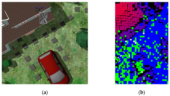
Figure 6. Illustration of ${\mathrm{v}}_{ucc}$ and ${\mathrm{v}}_{icc}$ in the visible area: (a) drone position and camera viewpoint in the simulation environment; and (b) corresponding $\mathit{M}$ segment according to the drone position. Unmapped cells are represented as white cells. Inaccurate cells are represented as green cells.

The variance of visible inaccurate cells (${\sigma }_m$) is obtained from the Bayes inference defined in (10), whereas that of visible unmapped cells $\left({\sigma }_k\right)$ is calculated from height deviations for the visible area ${\mathit{\xi }}_{\mathit{k}}$ as follows:

$${\sigma }_k=CalculateSigma\left(\mathit{M},{\mathit{\xi }}_k\right).$$

(25)

• As stated in (P-ii), if the planner algorithm runs periodically every $rT$ seconds, where r is the planning iteration, and T is the sampling period, while the drone flies at a constant speed, then the cost function given in (15) of the NBV planner becomes ineffective. Here, we solve (P-ii) by using the number of nodes between the subject node and the root node as the path cost instead of (15). Together with the new path cost and the information gain, the new gain function for RRT nodes to determine the best branch in Algorithm 3 in steps 21 and 23 is constructed as follows:

$$Gain\left(n_k,\lambda \right)=Gain\left(n_{k-1}\right)+InformationGain\left(\mathit{M},{\mathit{\xi }}_k\right)e^{-\lambda \eta }.$$

(26)

In (26), $\eta$ is the path cost representing the number of nodes between the root and the subject node, and $\lambda >0$ determines the behavior of the path cost. To test our proposal, let us handle the scenario again depicted in Figure 5. When the information contribution of visible unmapped and inaccurate cells in RRT Branch 1 is equal to that of both $n_3\left({\mathit{\xi }}_3\right)$ and $n_4({\mathit{\xi }}_4)$ in RRT Branch 2 as below:

$$InformationGain\left(\mathit{M},{\mathit{\xi }}_2\right)=InformationGain\left(\mathit{M},{\mathit{\xi }}_3\right)+InformationGain\left(\mathit{M},{\mathit{\xi }}_4\right)$$

(27)

then by using (26), the relation of node gain between $n_2({\mathit{\xi }}_2)$ and $n_4({\mathit{\xi }}_4)$ becomes:

$$InformationGain\left(\mathit{M},{\mathit{\xi }}_2\right)e^{-\lambda 2}>InformationGain\left(\mathit{M},{\mathit{\xi }}_3\right)e^{-\lambda 2}+InformationGain\left(\mathit{M},{\mathit{\xi }}_4\right)e^{-\lambda 3}$$

(28)

$$Gain\left(n_2,\lambda \right)>Gain\left(n_4,\lambda \right).$$

(29)

As can be seen from (29), the QABV planner always decides in favor of the shorter branch by using the new gain function given in (26).

• For (P-iii), we propose updating $\lambda >0$ to dynamically change the path cost within (26) while $\mathit{M}$ is being generated or updated. This allows the QABV planner to reduce the distance traveled while maintaining map coverage as follows:

  ○

  When there are many areas to explore nearby the drone, the information contribution of the nodes in $\mathbb{T}$ increases. In this case, we increase λ to aggressively penalize long paths. This increases the focus of the drone to explore nearby information-rich areas. Additionally, the distance traveled reduces since closer paths are being followed.

  ○

  The information contribution of the nodes diminishes while the nearby areas are being explored. In this case, the drone should exit the area, but aggressive path cost prevents further exploration and causes the drone to get stuck. We decrease λ to prevent this situation so that the drone can reach information-rich areas at longer distances.

In this context, we handle the λ generation problem from a control-theoretic perspective. The proposed QABV planner, presented in Algorithm 3, can be seen as a system to be controlled via the hyperparameter λ (i.e., control signal) such that the best node gain ($g_{best}$) (i.e., output signal) results in a waypoint satisfying the presented effects. We propose 4 novel methods to be used in Algorithm 3 in steps 11, 12, 13, and 16 based on control system theory to regulate the proposed QABV planner. The proposed control methods are shown in Figure 7 and will be explained in the remaining part of this section.

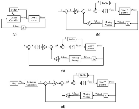
Figure 7. The proposed $\lambda$ updating methods for the QABV planner: (a) Method 1: on–off controller, (b) Method 2: PD controller, (c) Method 3: switching controller, and (d) Method 4: 2 DOF PD controller.

After obtaining the best branch of $\mathbb{T}$ via (22) and (26), the change in the best node gain $\left(g_{best}\right)$ is stored in Algorithm 3 in step 28 to be used in the proposed λ update methods in the next planning iterations. Then, the first waypoint of the branch to the best node $\mathit{w}\mathit{p}$ is determined with $ExtractBestPathWaypoint\left(n_{best}\right)$ and returned to the drone position controller, where $n_{best}$ is the node with the highest gain. The rest of the branch is used for initializing $\mathbb{T}$ after the first iteration. The creation of $\mathbb{T}$ is stopped at $N_{\mathbb{T}}=N_{max}$ in general, but if the best gain $g_{best}$ remains zero, tree construction is continued until $g_{best}>0$. The QABV planner depends on the generation of the probabilistic sparse elevation map, and it is terminated when Algorithm 1 finishes. Therefore, $N_{TOL}$ in Algorithm 2 is not used in the termination of the exploration.

The computational complexity of Algorithm 3 is dependent on the number of nodes $N_{\mathbb{T}}$ for RRT creation, the distance between adjacent nodes for collision checking, and the visible map segment ${\mathit{M}}^v$, which is centered at the drone position and proportional to the flight altitude for the node gain calculations. The complexity of the λ update methods is insignificant compared to the rest of the algorithm, and it will be mentioned in the remaining part of this section. The RRT creation complexity is $\mathcal{O}\left(N_{\mathbb{T}}log\left(N_{\mathbb{T}}\right)\right)$ as is in the NBV planner, and the query of the best node is $\mathcal{O}\left(N_{\mathbb{T}}\right)$. The complexity of a single query to $\mathit{M}$ is $\mathcal{O}\left(1\right)$ because the presented map in Section 2 stores data in a 2D matrix, and positions are encoded into matrix indexes as $\mathit{M}\left[\mathit{x}\right]\left[\mathit{y}\right]$. The collision check complexity for $N_{\mathbb{T}}-1$ path in the RRT is $\mathcal{O}\left(N_{\mathbb{T}}siz{e}_{{\mathit{M}}^p}\right)$, where $siz{e}_{{\mathit{M}}^p}$ is the size of a rectangle map segment with adjacent nodes in diagonal vertices. For node gain calculations of the RRT, the number of queries to $\mathit{M}$ is equal to the size of ${\mathit{M}}^v$ $\left(siz{e}_{{\mathit{M}}^v}\right)$. For visibility, a rectangle area with drone and subject positions in diagonal vertices is checked, and in the worst case, the number of queries to $\mathit{M}$ is equal to the size of ${\mathit{M}}^v$($siz{e}_{{\mathit{M}}^v}/4$) when checking for edges of ${\mathit{M}}^v$. So, the complexity of gain calculation for one node is $\mathcal{O}\left({\left(siz{e}_{{\mathit{M}}^v}\right)}^2/4\right)$. As a result, the total complexity of a single planning iteration is the sum of tree construction, collision check, and gain computation as follows:

$$\mathcal{O}(N_{\mathbb{T}}log\left(N_{\mathbb{T}}\right)+N_{\mathbb{T}}siz{e}_{{\mathit{M}}^p}+N_{\mathbb{T}}{\left(siz{e}_{{\mathit{M}}^v}\right)}^2/4).$$

(30)

3.2.1. λ Update Method 1: On–Off Controller Approach

As shown in Figure 7a, Method 1 acts like an on–off controller [32] to generate λ; however, rather than using an error signal, the QABV planner with Method 1 (QABV-1) observes $\mathsf{\Delta }{g}_{best}$ to understand if the information contribution of the area is increasing or decreasing and updates λ according to our update strategy as presented in Algorithm 4. $\mathsf{\Delta }{g}_{best}$ is calculated with the backward difference method:

$$\mathsf{\Delta }{g}_{best}=g_{best}-{\acute{g}}_{best}$$

(31)

in Algorithm 3 step 27, where ${\acute{g}}_{best}$ is the previous $g_{best}$ value from the previous planning iteration. Based on $\mathsf{\Delta }{g}_{best}$, QABV-1 increases λ when $\mathsf{\Delta }{g}_{best}>0$:

$${\lambda }_{new}=K\lambda .$$

(32)

On the other hand, when $\mathsf{\Delta }{g}_{best}<0$, QABV-1 decreases λ:

$${\lambda }_{new}=\lambda /K,$$

(33)

the λ change rate can be adjusted by $K>1$. Every operation in Method 1 takes constant time, therefore the computational complexity is $\mathcal{O}\left(1\right)$.

Algorithm 4. Method 1: On–off controller

1: $Method1(\mathsf{\Delta }{\mathit{g}}_{\mathit{b}\mathit{e}\mathit{s}\mathit{t}},\lambda$) 2:       if $\mathrm{size}\left(\mathsf{\Delta }{\mathit{g}}_{\mathit{b}\mathit{e}\mathit{s}\mathit{t}}\right)>\mathbf{0}$ 3:         $\mathsf{\Delta }{g}_{best}\leftarrow \mathsf{\Delta }{\mathit{g}}_{\mathit{b}\mathit{e}\mathit{s}\mathit{t}}\left[\mathit{e}\mathit{n}\mathit{d}\right]$ 4:          if $\mathsf{\Delta }{g}_{best}>0$ 5:           ${\lambda }_{new}\leftarrow K\lambda$ 6:         else 7:           ${\lambda }_{new}\leftarrow \lambda /K$ 8:         end if 9:       else 10:            ${\lambda }_{new}\leftarrow \lambda$ 11:          end if 12: return ${\lambda }_{new}$

3.2.2. λ Update Method 2: PD Controller Approach

As shown in Figure 7b, rather than directly setting λ such as in Method 1, the QABV planner with Method 2 (QABV-2), updates λ as follows:

$${\lambda }_{new}=\lambda +\mathsf{\Delta }\lambda$$

(34)

where $\mathsf{\Delta }\lambda$ is generated via PD controller defined as:

$$\mathsf{\Delta }\lambda =K_{P}E+K_D\mathsf{\Delta }{\overline{g}}_{best}.$$

(35)

Here, $K_P$ and $K_D$ are the proportional and derivative gains of the PD controller, respectively. As shown in Figure 7b, the derivative action of the PD controller is placed in the feedback loop to eliminate derivative kicks [33], and is implemented with a moving average filter over the past $w$ values of $\mathsf{\Delta }{g}_{best}$ $\left(\mathsf{\Delta }{\mathit{g}}_{\mathit{b}\mathit{e}\mathit{s}\mathit{t}}\right)$ from previous planning iterations of the planner:

$$\mathsf{\Delta }{\overline{g}}_{best}=\frac{1}{w}{\displaystyle \sum }_{\begin{array}{c}h=0\\ \end{array}}^{w-1}\mathsf{\Delta }{\mathit{g}}_{\mathit{b}\mathit{e}\mathit{s}\mathit{t}}\left[end-h\right].$$

(36)

The proportional action of the PD controller is driven via the error signal E:

$$E=R-{\acute{g}}_{best},$$

(37)

where R is the desired information contribution value (i.e., the reference signal) so that the best nodes provide the expected information contribution in every planning iteration. Note that (34) and (35) can be also seen as the velocity form of a PI controller. In defining $R$ in (37), we need to consider:

• If the value of R is too big, then λ may become saturated at later stages of the map generation process. Because when the stop criterion is close to being met, there will be limited information available in the environment, so the drone may not be able to collect enough information and the PD controller keeps decreasing λ to elevate $g_{best}$ to a big R value until λ saturates.
• If R is too small, then the PD controller may increase λ excessively at the first stages of the map generation process. Because in the beginning, there is plenty of information to gather from the environment, and information gain is at its highest point, this situation can slow down the exploration process and even make the drone get stuck in the early stages.

The implementation of Method 2 is presented in Algorithm 5. Note that if ${\lambda }_{new}\le 0$, to satisfy $\lambda >0$, we set ${\lambda }_{new}$ to positive small value $ϵ$. The computational complexity is $\mathcal{O}\left(w\right)$ and is dependent on the filter size in (36).

Algorithm 5. Method 2: PD controller

1: $Method2({\acute{g}}_{best},\mathsf{\Delta }{\mathit{g}}_{\mathit{b}\mathit{e}\mathit{s}\mathit{t}},\lambda$) 2:     if $\mathrm{size}\left(\mathsf{\Delta }{\mathit{g}}_{\mathit{b}\mathit{e}\mathit{s}\mathit{t}}\right)\ge w$ 3:         calculate $\mathsf{\Delta }{\overline{g}}_{best}$ using (36) 4:         $E\leftarrow R-{\acute{g}}_{best}$ 5:         $\mathsf{\Delta }\lambda \leftarrow K_{P}E+K_D\mathsf{\Delta }{\overline{g}}_{best}$ 6:         ${\lambda }_{new}\leftarrow \lambda +\mathsf{\Delta }\lambda$ 7:         if ${\lambda }_{new}\le 0$ 8:             ${\lambda }_{new}\leftarrow ϵ$ 9:         end if 10:       else 11:             ${\lambda }_{new}\leftarrow \lambda$ 12:     end if 13: return ${\lambda }_{new}$

3.2.3. λ Update Method 3: Switching Controller Approach

The QABV Planner with Method 3 (QABV-3) is a variation of QABV-2 with the same computational complexity and can be seen as a switching controller as shown in Figure 7c. In Algorithm 6, we presented the implementation where $\mathsf{\Delta }{\overline{g}}_{best}$ is calculated in (36).

We defined two switching conditions:

• When $R>{\acute{g}}_{best}$, the proportional action in the forward loop is activated to update λ using (35). Because when $\mathsf{\Delta }{\overline{g}}_{best}$ is small, only derivative action cannot decrease λ fast enough, and the drone gets stuck in the information-poor area. The proportional action solves this problem by reducing λ proportionally to the magnitude of E.
• When $R<{\acute{g}}_{best}$, the proportional action is deactivated. Because, in this case, map exploration and accuracy will increase beyond the desired level, therefore, only a derivative action updates λ to allow extra information and stabilize $g_{best}$ as follows:

$$\mathsf{\Delta }\lambda =K_D\mathsf{\Delta }{\overline{g}}_{best}.$$

(38)

In this way, when there is a change in $g_{best}$, the derivative action updates λ as much as $\mathsf{\Delta }{\overline{g}}_{best}$ to change $g_{best}$ in the reverse direction. So, the best viewpoints collect a similar amount of information from the environment during map generation.

Note that, if ${\lambda }_{new}\le 0$, ${\lambda }_{new}$ is set to $ϵ>0$.

Algorithm 6. Method 3: Switching controller

1: $Method3({\acute{g}}_{best},\mathsf{\Delta }{\mathit{g}}_{\mathit{b}\mathit{e}\mathit{s}\mathit{t}},\lambda$) 2:         if $\mathrm{size}\left(\mathsf{\Delta }{\mathit{g}}_{\mathit{b}\mathit{e}\mathit{s}\mathit{t}}\right)\ge w$ 3:             calculate $\mathsf{\Delta }{\overline{g}}_{best}$ using (36) 4:             $E\leftarrow$ initialize with zero 5:             if $R>{\acute{g}}_{best}$ 6:                 $E\leftarrow R-{\acute{g}}_{best}$ 7:             end if 8:             $\mathsf{\Delta }\lambda \leftarrow K_{P}E+K_D\mathsf{\Delta }{\overline{g}}_{best}$ 9:             ${\lambda }_{new}\leftarrow \lambda +\mathsf{\Delta }\lambda$ 10:             if ${\lambda }_{new}\le 0$ 11:                 ${\lambda }_{new}\leftarrow ϵ$ 12:             end if 13:         else 14:                 ${\lambda }_{new}\leftarrow \lambda$ 15:         end if 16: return ${\lambda }_{new}$

3.2.4. λ Update Method 4: 2 DOF PD Controller Approach

As shown in Figure 7d, rather than keeping R as a constant, the QABV planner with Method 4 (QABV-4) generates R dynamically while the map is generated via:

$$R=R_{min}+\left(R_{max}-R_{min}\right)e^{-M_{Acc}/\tau }$$

(39)

where $M_{Acc}$ is the map accuracy of the current planning iteration and is defined in (14). The desired information contribution value R is decreased exponentially from $R_{max}$ to $R_{min}$ as $M_{acc}$ is increasing. The speed is determined by the exponential decay constant $\tau$, and lower $\tau$ values speed up the decay from $R_{max}$ to $R_{min}$ as shown in Figure 8.

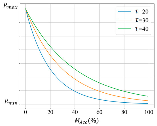
Figure 8. R against $M_{Acc}$ with different decay constants.

The motivation behind using $M_{Acc}$ is to estimate the amount of information the drone can gather from the environment is as follows:

• In the first planning iterations, the drone can gather maximum information from the environment as there is no prior information on the map and $M_{Acc}$ is zero. That is why we prefer a big $R$ value in the first planning iteration and set it to $R_{max}$, which is equal to the value of $g_{best}$ in the first planning iteration.
• As we progress through the planning iterations and represent the gathered information on the map, $M_{Acc}$ increases. As a result, available information in the environment becomes limited; therefore, we gradually decrease $R$ until it reaches its minimum value, $R_{min}$, towards the end of the map generation process.

In Algorithm 7, we presented the implementation of Method 4. Here,$E$ is defined in (37) and calculated with R as defined in (39). λ is updated using (35) after calculating $\mathsf{\Delta }{\overline{g}}_{best}$ via (36). Similarly, if ${\lambda }_{new}\le 0$, ${\lambda }_{new}$ is set to $ϵ>0$. When calculating the computational complexity, notice that the precalculated $M_{Acc}$ is obtained from the proposed map in Section 2. So, the complexity of Method 4 is the same as Methods 2 and 3.

Algorithm 7. Method 4: 2 DOF PD controller

1: $Method4\left({\acute{g}}_{best},\mathsf{\Delta }{\mathit{g}}_{\mathit{b}\mathit{e}\mathit{s}\mathit{t}},\lambda ,M_{Acc}\right)$ 2:     if $\mathrm{size}\left(\mathsf{\Delta }{\mathit{g}}_{\mathit{b}\mathit{e}\mathit{s}\mathit{t}}\right)\ge w$ 3:         calculate $\mathsf{\Delta }{\overline{g}}_{best}$ using (36) 4:         $R\leftarrow R_{min}$ + $\left(R_{max}-R_{min}\right)e^{-M_{Acc}/\tau }$ 5:         $E\leftarrow R-{\acute{g}}_{best}$ 6:         $\mathsf{\Delta }\lambda \leftarrow K_{P}E+K_D\mathsf{\Delta }{\overline{g}}_{best}$ 7:         ${\lambda }_{new}\leftarrow \lambda +\mathsf{\Delta }\lambda$ 8:         if ${\lambda }_{new}\le 0$ 9:             ${\lambda }_{new}\leftarrow ϵ$ 10:         end if 11:     else 12:         ${\lambda }_{new}\leftarrow \lambda$ 13:     end if 14: return ${\lambda }_{new}$

4. Comparative Performance Analysis

In this section, to validate our proposed approach and show its superiority, we present comparative experimental results. All experiments were conducted in Gazebo [34] simulation environment and the test drone used in the environment is specified in Table 1. The test drone has a down-looking camera that is used by SVO for position estimation and the creation of the point cloud. Figure 9 shows the simulation environment alongside a sample snapshot from the down-looking camera.

Table 1. Specifications of the simulation environment.

Drone Specifications
Motor-to-motor dimension	550 mm
Height	100 mm
Weight (with battery)	1282 g
Propellers	(2) 10 × 4.7 normal-rotation (2) 10 × 4.7 reverse-rotation
Motors	AC 2830, 850 kV
Camera Specifications
Image width	752 pixels
Image height	480 pixels
Image format	Black and white
Horizontal FOV	115 degrees
Update rate	20 Hz
Simulation Environment Apecifications for Rendering
Near clip plane	0.05
Far clip plane	15,000

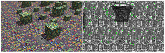
Figure 9. The test drone flies at a 2 m altitude in the simulation environment on the left side. On the right side, a sample picture captured by the down-looking camera is shown. The camera can see a 4 m × 6.2 m ground area at a 2 m altitude. Green points in the picture are corner features that are measured by SVO for position estimation and point cloud data.

The performance of the NBV planner and our proposal QABV planner are tested against 3 different maps shown in Figure 10. To compare the performances of the planners, the following criteria are used:

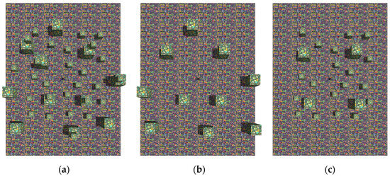
Figure 10. Test maps in Gazebo simulation environment: (a) map 1; (b) map 2; and (c) map 3. In the maps, cubes with side lengths of 1 m and 0.5 m are put on a flat surface with different positions, and each map is 18.6 m × 12 m in size.

• Map exploration as defined in (13);
• Map accuracy as defined in (14);
• Distance traveled to indicate the path length followed by the drone during the execution of Algorithm 1.

To consider the random behavior of RRT and to have a general understanding of the performance of the planners, all tests are repeated three times for each map.

In the test scenarios, the drone flies at a 2 m constant height on the XY plane in the map. ArduPilot flight controller [10] is used for the position controller of the drone and position estimations are supported by SVO. In our simulation studies, there was a need for the closed-loop system model since both planners require a system model of the drone to generate a feasible node tree considering the dynamic and kinematic constraints on the XY plane. In this context, we performed a naïve system identification experiment with a sampling (i.e., planning) period $T=3\mathrm{s}$ and fixed the linear velocity $V=0.2\mathrm{m}/\mathrm{s}$. The XY dynamics are obtained via the system identification toolbox of Matlab^® [35] and are as follows:

$$X\left(t\right)\cong 0.9944X\left(t-1\right)+9.197\times {10}^{-12}X\left(t-2\right)+2.86U_x\left(t-1\right)+0.1169U_x\left(t-2\right),U_x\left(t\right)=Vcos\theta \left(t\right)$$

(40)

$$Y\left(t\right)\cong 0.9968Y\left(t-1\right)+3.209\times {10}^{-15}Y\left(t-2\right)+2.894U_y\left(t-1\right)+0.08926U_y\left(t-2\right),U_y\left(t\right)=Vsin\theta \left(t\right),$$

(41)

where $\theta \left(t\right)$ is the yaw angle $(-\pi <\theta <\pi )$.

4.1. NBV Planner Results

NBV planner focuses on map exploration and does not consider map accuracy as given in (16). Thus, we defined the stop criterion as 95% map exploration. Additionally, as an enhancement to the NBV planner and for a fair comparison, we used the map representation defined in Section 2 instead of the occupancy map in the original study [20].

In Table 2, the averaged test results are shown for each map when $\lambda$ in (16) is set as 0.5. On average, the drone travels 79.29 m to explore 95% of the map and 74.2% of the explored map is accurate according to Bayes inference defined in (10) in Section 2 with SVO point cloud measurements.

Table 2. Experiment results for the NBV planner.

Performance Criteria	Map 1	Map 2	Map 3	Average
Map Exploration (%)	95.00	95.00	95.00	95.00
Map Accuracy (%)	72.00	73.00	77.70	74.20
Distance Traveled (m)	82.60	73.50	81.76	79.29

To obtain more insight into the NBV planner, we can look at the test result in Figure 11. The resultant elevation map from the top view is shown in Figure 11a. Although inaccurate cells also need to be visited again to become accurate with Bayes inference, the path created by the planner focuses on only exploring empty cells. Furthermore, the drone got stuck as mentioned in (P-iii). Because in Figure 11b, map exploration, and accuracy remain stable at iterations between 70 and 100, and a tangle occurs in Figure 11c. This results in low $g_{best}$, as we can see from Figure 11d, and the drone stays at the local minimum until the local minimum gain drops off.

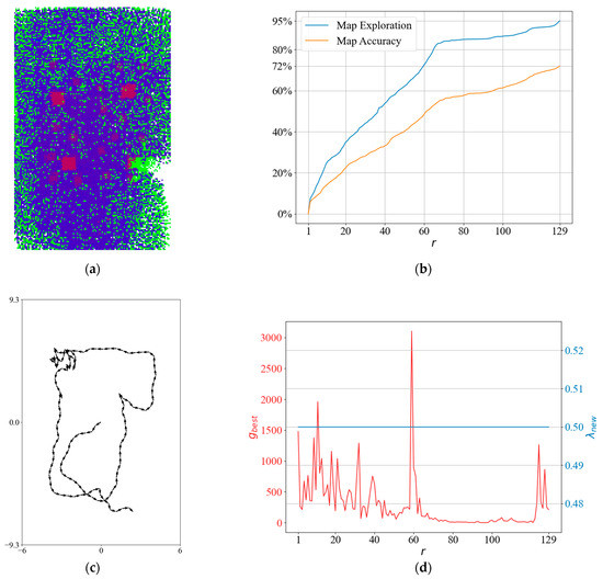
Figure 11. A detailed result for the NBV planner: (a) generated sparse elevation map (top view); (b) map rxploration and map accuracy; (c) the planned path; and (d) $g_{best}$ and $\lambda$.

4.2. QABV-1 Planner Results

The QABV-1 planner focuses on map accuracy and exploration at the same time as given in (22) and (26) in Section 3, so the stop criteria are chosen as 75%, 80%, and 85% map accuracy as defined in (14). We set ${\lambda }_{init}$ in Algorithm 3 to the same $\lambda$ value of NBV as ${\lambda }_{init}=0.5$.

In the QABV-1 planner tests, we examined how $K$ is affecting the performance by analyzing the results for $K\in \left\{1.2,1.3,1.4\right\}.$ Table 3, Table 4 and Table 5 show the averaged test results for each test map and each $K$ value. As can be seen from the results, the drone generally travels more in Map 1 to achieve similar results in other maps. The reason for this behavior can be explained by the number and different positions of the cubes. Because of the nature of the camera view angle, cubes occlude the area behind if they are intercepting the line of sight of the camera. The planner finds alternative routes for those occluded areas which naturally causes longer distance traveled.

Table 3. QABV-1 planner test results for $K=1.2$.

Performance Criteria		Map 1	Map 2	Map 3	Average
Map Accuracy 75%	Map Exploration (%)	96.60	93.60	93.25	94.48
	Distance Traveled (m)	68.03	64.45	57.15	63.21
Map Accuracy 80%	Map Exploration (%)	96.80	96.80	95.25	96.28
	Distance Traveled (m)	87.00	71.94	67.06	75.33
Map Accuracy 85%	Map Exploration (%)	98.50	97.75	96.50	97.58
	Distance Traveled (m)	101.48	83.85	73.35	86.23

Table 4. QABV-1 planner test results for $K=1.3$.

Performance Criteria		Map 1	Map 2	Map 3	Average
Map Accuracy 75%	Map Exploration (%)	95.00	93.33	91.66	93.33
	Distance Traveled (m)	63.59	68.13	68.28	66.67
Map Accuracy 80%	Map Exploration (%)	97.20	97.00	95.50	96.57
	Distance Traveled (m)	81.55	73.15	73.00	75.90
Map Accuracy 85%	Map Exploration (%)	98.60	98.00	97.66	98.09
	Distance Traveled (m)	91.50	94.37	77.15	87.67

Table 5. QABV-1 planner test results for $K=1.4$.

Performance Criteria		Map 1	Map 2	Map 3	Average
Map Accuracy 75%	Map Exploration (%)	95.00	94.80	89.00	92.93
	Distance Traveled (m)	82.8	59.21	59.69	67.23
Map Accuracy 80%	Map Exploration (%)	97.20	95.00	95.33	95.84
	Distance Traveled (m)	95.24	74.00	69.70	79.65
Map Accuracy 85%	Map Exploration (%)	98.60	97.25	97.00	97.62
	Distance Traveled (m)	119.55	85.29	87.82	97.55

To compare the performance of the QABV-1 planner against different $K$ values, we qabv-1can look at the average performance of the method on the test maps. In Figure 12, the average performances of map exploration and distance traveled are presented. Map accuracy is the stop criterion, which is why it is the same for all test cases. As can be seen from the figure, QABV-1 performs better with $K=1.2$ because the drone travels less while having a better map exploration on average compared to $K=1.3$ and $K=1.4$.

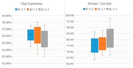
Figure 12. Analyzing test results for different hyperparameters for QABV-1 planner. Average map exploration and distance traveled from 75%, 80%, and 85% map accuracy test results are shown.

To obtain more insight into the QABV-1 planner, we can look at the test result in Figure 13 when $K=1.2$ and the stop criterion is 75% map accuracy. The resultant elevation map is shown in Figure 13a. Notice that QABV-1 is updating $\lambda$ during map exploration differently than NBV. Although the drone stays in a low-gain area during iterations between 70 and 100 because map statistics remain stable in Figure 13b, and a tangle occurs in the followed path in Figure 13c, QABV-1 decreases $\lambda$ to escape from the low-gain area and go to high-gain areas at a longer distance. After that, QABV-1 starts to increase $\lambda$ to reduce the distance traveled. After iteration 70, $\lambda$ is decreased according to the decreasing $g_{best}$ value and is increased again after iteration 100 with the increasing $g_{best}$ value (See Figure 13d).

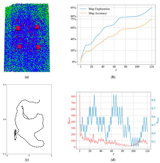
Figure 13. A detailed result of the QABV-1 planner: (a) generated sparse elevation map (top view); (b) map exploration and map accuracy; (c) the planned path when $K=1.2$; and (d) $g_{best}$ and $\lambda$.

4.3. QABV-2 Planner Results

In the QABV-2 planner tests, we set the moving average filter size as $w=5$, ${\lambda }_{init}=0.5$, and $K_P=-0.0001$ and $K_D=0.001$ to scale with the magnitude of $E$ and $\mathsf{\Delta }{\overline{g}}_{best}$ in (35). Note that we set $K_P<0$ as there is an inverse relation between $\lambda$ and $g_{best}$. We examined the performance for $R\in \left\{200,300\right\}$. Table 6 and Table 7 show the averaged test results for test maps.

Table 6. QABV-2 planner test results for $R=200$.

Performance Criteria		Map 1	Map 2	Map 3	Average
Map Accuracy 75%	Map Exploration (%)	95.67	93.33	91.66	93.55
	Distance Traveled (m)	62.81	65.27	59.12	62.40
Map Accuracy 80%	Map Exploration (%)	97.33	94.66	94.66	95.55
	Distance Traveled (m)	75.56	79.75	71.65	75.65
Map Accuracy 85%	Map Exploration (%)	98.00	98.66	96.00	97.55
	Distance Traveled (m)	102.5	84.18	83.08	89.92

Table 7. QABV-2 planner test results for $R=300$.

Performance Criteria		Map 1	Map 2	Map 3	Average
Map Accuracy 75%	Map Exploration (%)	95.67	94.33	93.67	94.56
	Distance Traveled (m)	57.45	56.00	52.61	55.35
Map Accuracy 80%	Map Exploration (%)	97.00	96.50	95.00	96.17
	Distance Traveled (m)	73.79	77.13	78.10	76.34
Map Accuracy 85%	Map Exploration (%)	97.67	98.00	96.67	97.45
	Distance Traveled (m)	93.18	80.66	91.55	88.46

To compare the performance of the QABV-2 planner against different $R$ values, we can look at the average performance of the method on the test maps. In Figure 14, the average performance of map exploration and distance traveled are shown. As can be seen from the figure, QABV-2 performs better with $R=300$ because the drone travels less while having more map exploration on average compared to $R=200$.

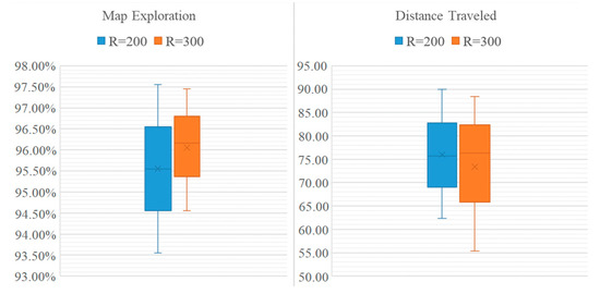
Figure 14. Analyzing test results for different hyperparameters for QABV-2 planner. Average map exploration and distance traveled from 75%, 80%, and 85% map accuracy test results are shown.

To obtain more insight into the QABV-2 planner, we can look at the test result in Figure 15 when $R=300$ and the stop criterion is 75% map accuracy. The resultant elevation map from the top view is shown in Figure 15a. Notice that QABV-2 updates $\lambda$ more smoothly by using a PD controller than QABV-1 in Figure 13. On the other hand, QABV-2 waits before updating $\lambda$ more than QABV-1 until enough information is gathered because of the moving average filter that is defined in (36) in Section 3.2.2; however, QABV-1 only waits for the calculation of $\mathsf{\Delta }{g}_{best}$ and starts updating $\lambda$ in the third iteration.

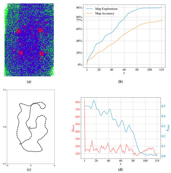
Figure 15. A detailed result of the QABV-2 planner: (a) generated sparse elevation map (top view); (b) map exploration and map accuracy; (c) the planned path when $R=300$; and (d) $g_{best}$ and $\lambda$.

4.4. QABV-3 Planner Results

In the QABV-3 planner tests, we used the same values as the QABV-2 planner tests. Table 8 and Table 9 show the averaged test results for each test map and each $R$ value.

Table 8. QABV-3 planner test results for $R=200$.

Performance Criteria		Map 1	Map 2	Map 3	Average
Map Accuracy 75%	Map Exploration (%)	94.00	94.66	93.00	93.89
	Distance Traveled (m)	68.41	54.86	53.62	58.96
Map Accuracy 80%	Map Exploration (%)	97.33	96.00	95.33	96.22
	Distance Traveled (m)	75.18	66.16	63.27	68.20
Map Accuracy 85%	Map Exploration (%)	97.33	97.33	98.00	97.55
	Distance Traveled (m)	89.76	95.88	89.62	91.75

Table 9. QABV-3 planner test results for $R=300$.

Performance Criteria		Map 1	Map 2	Map 3	Average
Map Accuracy 75%	Map Exploration (%)	96.00	95.00	94.00	95.00
	Distance Traveled (m)	55.30	52.12	56.70	54.71
Map Accuracy 80%	Map Exploration (%)	97.00	96.33	94.33	95.89
	Distance Traveled (m)	66.46	62.78	71.31	66.85
Map Accuracy 85%	Map Exploration (%)	97.66	96.66	96.00	96.77
	Distance Traveled (m)	77.90	87.43	89.42	84.92

To compare the performance of the QABV-3 planner against different $R$ values, we can look at the average performance of the method on the test maps. In Figure 16, the average performance of map exploration and distance traveled are shown. As can be seen from the figure, QABV-3 performs better with $R=300$ because the drone travels less while having more map exploration on average compared to $R=200$.

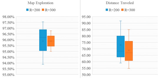
Figure 16. Analyzing test results for different hyperparameters for QABV-3 planner. Average map exploration and distance traveled from 75%, 80%, and 85% map accuracy test results are shown.

To obtain more insight into the QABV-3 planner, we can look at the test result in Figure 17 when $R=300$ and the stop criterion is 75% map accuracy. The resultant elevation map from the top view is shown in Figure 17a. Notice that QABV-3 allows for $g_{best}>R$ with its switching controller compared to QABV-2 in Figure 15.

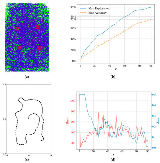
Figure 17. A detailed result of the QABV-3 planner: (a) generated sparse elevation map (top view); (b) map exploration and map accuracy; (c) the planned path when $R=300$; and (d) $g_{best}$ and λ.

4.5. QABV-4 Planner Results

In the QABV-4 tests, we set $R_{max}=1000$ and examined the performance for $R_{min}\in \left\{200,300\right\}$ and $\tau \in \left\{20,30,40\right\}$. The remaining parameters are set to the same values as QABV-3. Table 10 and Table 11 show the results for $R_{min}=200$ and $R_{min}=300$, respectively.

Table 10. QABV-4 planner test results for $R_{min}=200$.

Decay Constant	Performance Criteria		Map 1	Map 2	Map 3	Average
τ = 20	Map Accuracy 75%	Map Exploration (%)	95.00	94.00	95.00	94.67
		Distance Traveled (m)	71.99	64.82	62.52	66.44
	Map Accuracy 80%	Map Exploration (%)	96.60	96.00	96.00	96.20
		Distance Traveled (m)	73.53	72.56	71.67	72.59
	Map Accuracy 85%	Map Exploration (%)	98.00	98.60	97.60	98.07
		Distance Traveled (m)	95.78	88.61	86.86	90.42
τ = 30	Map Accuracy 75%	Map Exploration (%)	93.66	93.00	95.33	94.00
		Distance Traveled (m)	67.87	64.78	62.52	65.06
	Map Accuracy 80%	Map Exploration (%)	96.00	93.66	96.33	95.33
		Distance Traveled (m)	92.26	88.13	71.67	84.02
	Map Accuracy 85%	Map Exploration (%)	98.33	98.33	97.66	98.11
		Distance Traveled (m)	96.18	100.1	86.86	94.38
τ = 40	Map Accuracy 75%	Map Exploration (%)	95.66	93.33	91.33	93.44
		Distance Traveled (m)	69.37	60.07	64.12	64.52
	Map Accuracy 80%	Map Exploration (%)	95.66	96.33	95.00	95.66
		Distance Traveled (m)	72.24	70.76	71.56	71.52
	Map Accuracy 85%	Map Exploration (%)	97.33	97.66	95.66	96.88
		Distance Traveled (m)	94.74	86.67	85.76	89.06

Table 11. QABV-4 planner test results for $R_{min}=300$.

Decay Constant	Performance Criteria		Map 1	Map 2	Map 3	Average
τ = 20	Map Accuracy 75%	Map Exploration (%)	93.00	92.33	92.00	92.44
		Distance Traveled (m)	70.36	62.40	60.00	64.25
	Map Accuracy 80%	Map Exploration (%)	96.00	96.33	93.66	95.33
		Distance Traveled (m)	80.94	78.72	69.45	76.37
	Map Accuracy 85%	Map Exploration (%)	97.33	97.00	96.00	96.78
		Distance Traveled (m)	93.29	97.04	78.58	89.64
τ = 30	Map Accuracy 75%	Map Exploration (%)	96.33	95.66	94.00	95.33
		Distance Traveled (m)	50.39	56.61	57.08	54.69
	Map Accuracy 80%	Map Exploration (%)	96.33	95.33	96.00	95.89
		Distance Traveled (m)	70.5	73.19	68.6	70.76
	Map Accuracy 85%	Map Exploration (%)	98.00	98.20	97.00	97.73
		Distance Traveled (m)	107.6	92.61	76.35	92.19
τ = 40	Map Accuracy 75%	Map Exploration (%)	94.33	94.00	93.00	93.70
		Distance Traveled (m)	69.81	58.06	61.81	63.23
	Map Accuracy 80%	Map Exploration (%)	96.00	95.00	95.00	95.33
		Distance Traveled (m)	78.95	78.71	69.51	75.72
	Map Accuracy 85%	Map Exploration (%)	97.66	97.66	97.00	97.44
		Distance Traveled (m)	93.02	82.93	86.56	87.50

To compare the performance of the QABV-4 planner with different $R_{min}$ and $\tau$ settings, we can examine the average performances presented in Figure 18. As can be seen, QABV-4 performs better with $R_{min}=300$ and $\tau =30$ since the drone travels less while having more map exploration on average than other combinations.

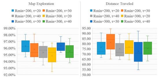
Figure 18. Analyzing test results for different hyperparameters for QABV-4 planner. Average map exploration and distance traveled for 75%, 80%, and 85% map accuracy test results are shown.

To obtain more insight into the QABV-4 planner, we can look at the test result in Figure 19 when $R_{min}=300$, $\tau =30,$ and the stop criterion is 75% map accuracy. The resultant elevation map from the top view is shown in Figure 19a. In Figure 19b, notice that map exploration and accuracy remain stable at iterations between 70 and 100 because in Figure 19c, we can see that the planned path is overlapping. In Figure 19d, notice that λ is decreased at the same iterations to keep $g_{best}$ at $R$. Also notice that λ is not increased at the first iterations as is in QABV-2 in Figure 15d because $R$ is set to $R_{max}$ at the first iteration according to (39) in Section 3.2.4, and λ is decreased to elevate $g_{best}$. On the other hand, in the QABV-2 test, $R$ is set to 300, and λ is increased to reduce $g_{best}$.

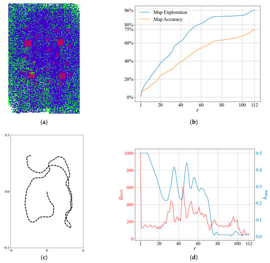
Figure 19. A detailed result of the QABV-4 planner: (a) generated sparse elevation map (top view); (b) map exploration and map accuracy; (c) the planned path when $R_{min}=300,\tau =30$; and (d) $g_{best}$ and λ.

4.6. Overall Performance Comparison

To make an overall performance comparison, we tabulate the baseline NBV planner results against the best resulting QABV planners which are:

• QABV-1 when $K=1.2$;
• QABV-2 when $R=300,K_P=-0.0001,K_D=0.001,w=5$;
• QABV-3 when $R=300,K_P=-0.0001,K_D=0.001,w=5$;
• QABV-4 when $R_{max}=1000,R_{min}=300,\tau =30,K_P=-0.0001,K_D=0.001,w=5$.

As tabulated in Table 12, when the test stop criterion is 75% map accuracy, the QABV planner significantly reduces the distance traveled compared to the NBV planner:

Table 12. Baseline NBV planner performance results against the best resulting QABV planners.

Planner	Performance Criteria	Map 1	Map 2	Map 3	Average
NBV planner	Map Accuracy (%)	72.00	73.00	77.70	74.20
	Map Exploration (%)	95.00	95.00	95.00	95.00
	Distance Traveled (m)	82.60	73.50	81.76	79.29
QABV-1 planner	Map Accuracy (%)	75.00	75.00	75.00	75.00
	Map Exploration (%)	96.60	93.60	93.25	94.48
	Distance Traveled (m)	68.03	64.45	57.15	63.21
QABV-2 planner	Map Accuracy (%)	75.00	75.00	75.00	75.00
	Map Exploration (%)	95.67	94.33	93.67	94.56
	Distance Traveled (m)	57.45	56.00	52.61	55.35
QABV-3 planner	Map Accuracy (%)	75.00	75.00	75.00	75.00
	Map Exploration (%)	96.00	95.00	94.00	95.00
	Distance Traveled (m)	55.30	52.12	56.70	54.71
QABV-4 planner	Map Accuracy (%)	75.00	75.00	75.00	75.00
	Map Exploration (%)	96.33	95.66	94.00	95.33
	Distance Traveled (m)	50.39	56.61	57.08	54.69

• 20.28% less distance traveled using QABV-1;
• 30.19% less distance traveled using QABV-2;
• 31% less distance traveled using QABV-3;
• 31.02% less distance traveled using QABV-4;

while having negligible differences in map exploration and accuracy.

From the results presented in Table 13, when the test stop criterion is 80% map accuracy, the QABV planner continues to reduce the distance traveled although 7.8% more map accuracy is being asked compared to the NBV planner:

Table 13. The best resulting QABV planners with stop criteria of 80% and 85% map accuracy.

Planner	Performance Criteria		Map 1	Map 2	Map 3	Average
QABV-1 planner	Map Accuracy 80%	Map Exploration (%)	96.80	96.80	95.25	96.28
		Distance Traveled (m)	87.00	71.94	67.06	75.33
	Map Accuracy 85%	Map Exploration (%)	98.50	97.75	96.50	97.58
		Distance Traveled (m)	101.48	83.85	73.35	86.23
QABV-2 planner	Map Accuracy 80%	Map Exploration (%)	97.00	96.50	95.00	96.17
		Distance Traveled (m)	73.79	77.13	78.10	76.34
	Map Accuracy 85%	Map Exploration (%)	97.67	98.00	96.67	97.45
		Distance Traveled (m)	93.18	80.66	91.55	88.46
QABV-3 planner	Map Accuracy 80%	Map Exploration (%)	97.00	96.33	94.33	95.89
		Distance Traveled (m)	66.46	62.78	71.31	66.85
	Map Accuracy 85%	Map Exploration (%)	97.66	96.66	96.00	96.77
		Distance Traveled (m)	77.90	87.43	89.42	84.92
QABV-4 planner	Map Accuracy 80%	Map Exploration (%)	96.33	95.33	96.00	95.89
		Distance Traveled (m)	70.5	73.19	68.6	70.76
	Map Accuracy 85%	Map Exploration (%)	98.00	98.20	97.00	97.73
		Distance Traveled (m)	107.6	92.61	76.35	92.19

• 5% less distance traveled using QABV-1;
• 3.72% less distance traveled using QABV-2;
• 15.69% less distance traveled using QABV-3;
• 10.76% less distance traveled using QABV-4;

while having negligible differences in map exploration; however, the distance traveled increases when the stop criterion is 85% map accuracy.

Lastly, to compare the performance of the dynamic λ update methods, Figure 20 visualizes the test results in Table 12 and Table 13 for average map exploration and distance traveled. Referring to the figure, the average map exploration is around 96% for each method, and QABV-4 performs slightly better than others; however, the average distance traveled differs between the methods, and QABV-3 performs significantly better than the others with 68.82 m. Although the map exploration performance of the QABV-4 is slightly better, its performance in reducing the distance traveled makes the QABV-3 to be the first choice of implementation. On the other hand, QABV-1 is the least performant method but the easiest to implement at the same time.

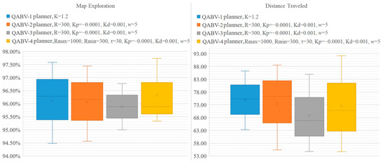
Figure 20. Analyzing test results for different QABV planner dynamic λ update methods. Average map exploration and distance traveled for 75%, 80%, and 85% map accuracy test results are shown.

5. A Real-World Scenario

To see the performance of the proposed planner in a real-world scenario such as delivering a package to a residential area, the map in Figure 21 is generated. In the scenario, the drone flies at a 5 m constant height on the x-y plane. Thus, the down-looking camera of the drone can see a broader area than before since the drone flight altitude is increased. Additionally, the distance between adjacent nodes in the RRT tree is increased in response to a broader visible area of the camera.

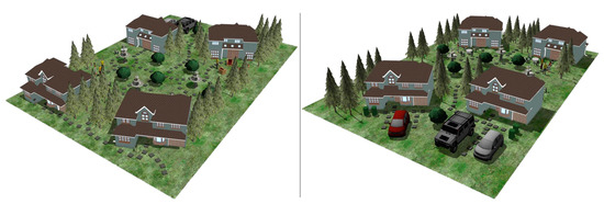
Figure 21. Test map for real-world scenario tests. The map is 37.2 m × 24 m in size, and it represents the backyard of the houses.

Table 14 shows test results when the stop criterion is 95% map exploration for the NBV planner and 75% map accuracy for the QABV planner. Tests are repeated for each dynamic λ update method with the same parameters as given in Section 4.6. Referring to Table 14, there is a noticeable increase in the average distance traveled results because of two main reasons. First, the map area is doubled, and second, big objects are causing occlusions for the camera; more specifically, the houses in the environment are affecting the visibility of the area behind since they are closer to the camera because of their height.

Table 14. Performance measures of NBV and QABV planners in real-world scenario test.

Performance Criteria	NBV Planner	QABV-1 Planner	QABV-2 Planner	QABV-3 Planner	QABV-4 Planner
Map Exploration (%)	95.00	95.00	95.50	95.50	95.50
Map Accuracy (%)	74.00	75.00	75.00	75.00	75.00
Distance Traveled (m)	276.34	216.41	205.90	200.88	203.29

When the planners are calculating the gain of the RRT nodes, the nodes nearby the houses obtain low gains because of the occlusion. That is why in Figure 22, we can see that the drone prefers to travel in the non-occluded area until the information depletes because in Figure 22a, the middle of the map is marked with blue cells indicating that the garden is relatively lower than other objects, and the drone prefers to stay in this region more as we can see from the tangles in the followed path in Figure 22c; however, when the drone finds itself in a low-information gain area, the dynamic cost function decreases λ and the QABV planner selects the nodes nearby the houses as the best viewpoints.

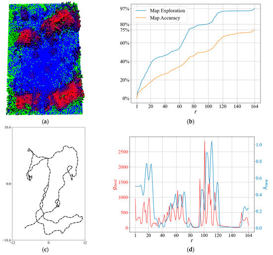
Figure 22. A detailed result of the QABV-3 planner in a real-world scenario: (a) generated sparse elevation map (top view); (b) map exploration and map accuracy; (c) the planned path when $R=300,k_{\mathit{p}}=0.0001,k_{\mathit{d}}=0.001,w=5$; and (d) $g_{best}$ and λ.

6. Conclusions and Future Work

In this study, we proposed a new terrain mapping and exploration system to be used for autonomous drone landings. For mapping, we presented the probabilistic sparse elevation map to enable the representation of sensor measurement error. For exploration, we presented the QABV planner for autonomous drone navigation with a dual focus: map exploration and quality. We showed that by exploiting the probabilistic nature of the proposed map with the novel information gain function, the QABV planner increases the measurement accuracy while exploring the map.

To reduce the distance traveled, we presented that using the node count as path cost is very effective in our scenario rather than the distance between adjacent nodes as was in the NBV planner. Furthermore, we presented four different control methods to dynamically adjust the path cost. We showed that the QABV planner can be seen as a system to be controlled via λ such that shorter paths are generated when the drone is in an information-rich area, or longer paths are allowed to exit from an information-poor area and to avoid getting stuck. In simulation studies, we tested our proposals against the NBV planner and verified their usefulness. In particular, QABV-3 and QABV-4 achieved superior results regarding the distance traveled and map quality. Although QABV-4 has slightly better map exploration performance, its performance in reducing the distance traveled makes the QABV-3 the first option for implementation.

One limitation of our proposed system is that the drone flies at a constant altitude while the probabilistic sparse elevation map is generated. This may limit the accuracy and resolution of the map, especially in areas with varying terrain or elevation. Another limitation is the use of hyperparameters in the λ update methods such as K, R, and $\tau$ which must be determined in a heuristic mannner. In the test results section, our analysis shows that the performance of the methods is sensitive to these parameters, and better-determined values can result in better performances.

As for our future work, we will focus on addressing these limitations by exploring adaptive control methods for generating elevation maps and automating the determination of hyperparameters. Furthermore, we plan to work on the proposed approach and deploy it in a real-world environment to examine how it performs in the presence of real-world uncertainties.

References

- Wang, S.; Han, Y.; Chen, J.; Zhang, Z.; Wang, G.; Du, N. A Deep-Learning-Based Sea Search and Rescue Algorithm by UAV Remote Sensing. In Proceedings of the 2018 IEEE CSAA Guidance, Navigation and Control Conference (CGNCC), Xiamen, China, 10–12 August 2018; IEEE: New York, NY, USA, 2018; pp. 1–5. [Google Scholar]
- Wang, C.; Liu, P.; Zhang, T.; Sun, J. The Adaptive Vortex Search Algorithm of Optimal Path Planning for Forest Fire Rescue UAV. In Proceedings of the 2018 IEEE 3rd Advanced Information Technology, Electronic and Automation Control Conference (IAEAC), Chongqing, China, 12–14 October 2018; IEEE: New York, NY, USA, 2018; pp. 400–403. [Google Scholar]
- Chen, S.; Meng, W.; Xu, W.; Liu, Z.; Liu, J.; Wu, F. A Warehouse Management System with UAV Based on Digital Twin and 5G Technologies. In Proceedings of the 2020 7th International Conference on Information, Cybernetics, and Computational Social Systems (ICCSS), Guangzhou, China, 13–15 November 2020; IEEE: New York, NY, USA, 2020; pp. 864–869. [Google Scholar]
- Liu, H.; Chen, Q.; Pan, N.; Sun, Y.; An, Y.; Pan, D. UAV Stocktaking Task-Planning for Industrial Warehouses Based on the Improved Hybrid Differential Evolution Algorithm. IEEE Trans. Ind. Inform. 2021, 18, 582–591. [Google Scholar] [CrossRef]
- Masmoudi, N.; Jaafar, W.; Cherif, S.; Abderrazak, J.B.; Yanikomeroglu, H. UAV-Based Crowd Surveillance in Post COVID-19 Era. IEEE Access 2021, 9, 162276–162290. [Google Scholar] [CrossRef]
- Song, H.; Yoo, W.-S.; Zatar, W. Interactive Bridge Inspection Research Using Drone. In Proceedings of the 2022 IEEE 46th Annual Computers, Software, and Applications Conference (COMPSAC), Alamitos, CA, USA, 27 June–1 July 2022; IEEE: New York, NY, USA, 2022; pp. 1002–1005. [Google Scholar]
- Worakuldumrongdej, P.; Maneewam, T.; Ruangwiset, A. Rice Seed Sowing Drone for Agriculture. In Proceedings of the 2019 19th International Conference on Control, Automation and Systems (ICCAS), Jeju, Republic of Korea, 15–18 October 2019; IEEE: New York, NY, USA, 2019; pp. 980–985. [Google Scholar]
- Raivi, A.M.; Huda, S.M.A.; Alam, M.M.; Moh, S. Drone Routing for Drone-Based Delivery Systems: A Review of Trajectory Planning, Charging, and Security. Sensors 2023, 23, 1463. [Google Scholar] [CrossRef] [PubMed]
- PX4 Autopilot. Available online: https://px4.io/ (accessed on 19 February 2023).
- ArduPilot. Available online: https://ardupilot.org/copter (accessed on 19 February 2023).
- Johnson, A.E.; Klumpp, A.R.; Collier, J.B.; Wolf, A.A. Lidar-Based Hazard Avoidance for Safe Landing on Mars. J. Guid. Control. Dyn. 2002, 25, 1091–1099. [Google Scholar] [CrossRef]
- Scherer, S.; Chamberlain, L.; Singh, S. Autonomous Landing at Unprepared Sites by a Full-Scale Helicopter. Robot. Auton. Syst. 2012, 60, 1545–1562. [Google Scholar] [CrossRef]
- Templeton, T.; Shim, D.H.; Geyer, C.; Sastry, S.S. Autonomous Vision-Based Landing and Terrain Mapping Using an MPC-Controlled Unmanned Rotorcraft. In Proceedings of the Proceedings 2007 IEEE International Conference on Robotics and Automation, Roma, Italy, 10–14 April 2007; IEEE: New York, NY, USA, 2007; pp. 1349–1356. [Google Scholar]
- Geyer, C.; Templeton, T.; Meingast, M.; Sastry, S.S. The Recursive Multi-Frame Planar Parallax Algorithm. In Proceedings of the Third International Symposium on 3D Data Processing, Visualization, and Transmission (3DPVT’06), Chapel Hill, NC, USA, 14–16 June 2006; IEEE: New York, NY, USA, 2006; pp. 17–24. [Google Scholar]
- Desaraju, V.R.; Michael, N.; Humenberger, M.; Brockers, R.; Weiss, S.; Nash, J.; Matthies, L. Vision-Based Landing Site Evaluation and Informed Optimal Trajectory Generation toward Autonomous Rooftop Landing. Auton. Robot. 2015, 39, 445–463. [Google Scholar] [CrossRef]
- Yang, T.; Li, P.; Zhang, H.; Li, J.; Li, Z. Monocular Vision SLAM-Based UAV Autonomous Landing in Emergencies and Unknown Environments. Electronics 2018, 7, 73. [Google Scholar] [CrossRef]
- Forster, C.; Faessler, M.; Fontana, F.; Werlberger, M.; Scaramuzza, D. Continuous On-Board Monocular-Vision-Based Elevation Mapping Applied to Autonomous Landing of Micro Aerial Vehicles. In Proceedings of the 2015 IEEE International Conference on Robotics and Automation (ICRA), Seattle, WA, USA, 26–30 May 2015; IEEE: New York, NY, USA, 2015; pp. 111–118. [Google Scholar]
- Forster, C.; Pizzoli, M.; Scaramuzza, D. SVO: Fast Semi-Direct Monocular Visual Odometry. In Proceedings of the 2014 IEEE international conference on robotics and automation (ICRA), Hong Kong, China, 31 May–5 June 2014; IEEE: New York, NY, USA, 2014; pp. 15–22. [Google Scholar]
- Delmerico, J.; Scaramuzza, D. A Benchmark Comparison of Monocular Visual-Inertial Odometry Algorithms for Flying Robots. In Proceedings of the 2018 IEEE international conference on robotics and automation (ICRA), Brisbane, Australia, 21–26 May 2018; IEEE: New York, NY, USA, 2018; pp. 2502–2509. [Google Scholar]
- Bircher, A.; Kamel, M.; Alexis, K.; Oleynikova, H.; Siegwart, R. Receding Horizon"next-Best-View" Planner for 3d Exploration. In Proceedings of the 2016 IEEE international conference on robotics and automation (ICRA), Stockholm, Sweden, 16–20 May 2016; IEEE: New York, NY, USA, 2016; pp. 1462–1468. [Google Scholar]
- Schmid, L.; Pantic, M.; Khanna, R.; Ott, L.; Siegwart, R.; Nieto, J. An Efficient Sampling-Based Method for Online Informative Path Planning in Unknown Environments. IEEE Robot. Autom. Lett. 2020, 5, 1500–1507. [Google Scholar] [CrossRef]
- Selin, M.; Tiger, M.; Duberg, D.; Heintz, F.; Jensfelt, P. Efficient Autonomous Exploration Planning of Large-Scale 3-d Environments. IEEE Robot. Autom. Lett. 2019, 4, 1699–1706. [Google Scholar] [CrossRef]
- Mittal, M.; Mohan, R.; Burgard, W.; Valada, A. Vision-Based Autonomous UAV Navigation and Landing for Urban Search and Rescue. In Proceedings of the Robotics Research: The 19th International Symposium ISRR, Hanoi, Vietnam, 6–10 October 2019; Springer: Cham, Switzerland, 2022; pp. 575–592. [Google Scholar]
- Zhang, Z.; Scaramuzza, D. Perception-Aware Receding Horizon Navigation for MAVs. In Proceedings of the 2018 IEEE International Conference on Robotics and Automation (ICRA), Brisbane, Australia, 21–26 May 2018; IEEE: New York, NY, USA, 2018; pp. 2534–2541. [Google Scholar]
- Davison, A.J.; Murray, D.W. Simultaneous Localization and Map-Building Using Active Vision. IEEE Trans. Pattern Anal. Mach. Intell. 2002, 24, 865–880. [Google Scholar] [CrossRef]
- Mueller, M.W.; Hehn, M.; D’Andrea, R. A Computationally Efficient Algorithm for State-to-State Quadrocopter Trajectory Generation and Feasibility Verification. In Proceedings of the 2013 IEEE/RSJ International Conference on Intelligent Robots and Systems, Tokyo, Japan, 3–7 November 2013; IEEE: New York, NY, USA, 2013; pp. 3480–3486. [Google Scholar]
- LaValle, S.M. Rapidly-Exploring Random Trees: A New Tool for Path Planning. Annu. Res. Rep. 1998. [Google Scholar]
- Karaman, S.; Frazzoli, E. Sampling-Based Algorithms for Optimal Motion Planning. Int. J. Robot. Res. 2011, 30, 846–894. [Google Scholar] [CrossRef]
- Yamauchi, B. A Frontier-Based Approach for Autonomous Exploration. In Proceedings of the 1997 IEEE International Symposium on Computational Intelligence in Robotics and Automation CIRA’97.’Towards New Computational Principles for Robotics and Automation, Monterey, CA, USA, 10–11 July 1997; IEEE: New York, NY, USA, 1997; pp. 146–151. [Google Scholar]
- Pizzoli, M.; Forster, C.; Scaramuzza, D. REMODE: Probabilistic, Monocular Dense Reconstruction in Real Time. In Proceedings of the 2014 IEEE International Conference on Robotics and Automation (ICRA), Hong Kong, China, 31 May–5 June 2014; IEEE: New York, NY, USA, 2014; pp. 2609–2616. [Google Scholar]
- Hornung, A.; Wurm, K.M.; Bennewitz, M.; Stachniss, C.; Burgard, W. OctoMap: An Efficient Probabilistic 3D Mapping Framework Based on Octrees. Auton. Robot. 2013, 34, 189–206. [Google Scholar] [CrossRef]
- Ogata, K. Two-Position or On–Off Control Action. In Modern Control Engineering; Prentice Hall: Upper Saddle River, NJ, USA, 2010; Volume 5, pp. 22–23. [Google Scholar]
- Ogata, K. PI-D Control. In Modern Control Engineering; Prentice Hall: Upper Saddle River, NJ, USA, 2010; Volume 5, pp. 590–591. [Google Scholar]
- Gazebo. Available online: https://gazebosim.org/home (accessed on 22 February 2023).
- System Identification Toolbox. Available online: https://nl.mathworks.com/products/sysid.html (accessed on 22 February 2023).
Disclaimer/Publisher’s Note: The statements, opinions and data contained in all publications are solely those of the individual author(s) and contributor(s) and not of MDPI and/or the editor(s). MDPI and/or the editor(s) disclaim responsibility for any injury to people or property resulting from any ideas, methods, instructions or products referred to in the content. |
© 2023 by the authors. Licensee MDPI, Basel, Switzerland. This article is an open access article distributed under the terms and conditions of the Creative Commons Attribution (CC BY) license (https://creativecommons.org/licenses/by/4.0/).