Abstract
The existence of information silos between vehicles and parking lots means that Unmanned Ground Vehicles (UGVs) repeatedly drive to seek available parking slots, resulting in wasted resources, time consumption and traffic congestion, especially in high-density parking scenarios. To address this problem, a novel UGV parking planning method is proposed in this paper, which consists of cooperative path planning, conflict resolution strategy, and optimal parking slot allocation, intending to avoid ineffective parking seeking by vehicles and releasing urban traffic pressure. Firstly, the parking lot induction model was established and the IACA–IA was developed for optimal parking allocation. The IACA–IA was generated using the improved ant colony algorithm (IACA) and immunity algorithm. Compared with the first-come-first-served algorithm (FCFS), the normal ant colony algorithm (NACA), and the immunity algorithm (IA), the IACA–IA was able to allocate optimal slots at a lower cost and in less time in complex scenarios with multi-entrance parking lots. Secondly, an improved conflict-based search algorithm (ICBS) was designed to efficiently resolve the conflict of simultaneous path planning for UGVs. The dual-layer objective expansion strategy is the core of the ICBS, which takes the total path cost of UGVs in the extended constraint tree as the first layer objective, and the optimal driving characteristics of a single UGV as the second layer objective. Finally, three kinds of load-balancing and unbalanced parking scenarios were constructed to test the proposed method, and the performance of the algorithm was demonstrated from three aspects, including computation, quality and timeliness. The results show that the proposed method requires less computation, has higher path quality, and is less time-consuming in high-density scenarios, which provide a reasonable and efficient solution for innovative urban mobility.
1. Introduction
The overabundance of vehicle ownership has led to a shortage of parking slots, making the challenge to find parking a key hot topic in today’s urban traffic [1]. The majority of parking areas that are subterranean, have vast areas, more storage space, and space constraints, are found in large retail malls, hospitals, parks, etc., and have poor security management [2,3]. There is a problem of prolonged queues and even deadlock for the vehicles that need to be parked. The current parking system generally reports the number of available slots, but is unable to pinpoint their exact position or rationally distribute parking slots or map out travel routes for vehicles. Vehicles may seek parking slots repeatedly if several vehicles attempt to park in the same slot. This causes congestion and has an emotional impact on drivers [4]. Therefore, we systematically take into account the traffic congestion that the multi-UGV-based parking system faces, and we make decisions starting from the selection of parking slots for vehicles, the best driving path, and then conflict resolution of multiple vehicles, starting as soon as the vehicles arrive at the entrance of the parking lot. This paper aims to provide each vehicle with a reasonable and efficient planning solution to fundamentally improve urban mobility and release urban traffic congestion.
1.1. Literature Review
1.1.1. Innovative Urban Parking Lot
The traditional unattended parking lot makes it typically difficult to have uniform vehicle entry and exit. The exit and entrance of the parking lot are prone to congestion, making it challenging to coordinate the sequence of vehicle entry and exit, notably during the peak commuter period. To keep a standard parking lot operating normally, a considerable amount of labor and material resources is required. This issue can be resolved using an intelligent vehicle and a parking guiding system. For instance, when there is heavy traffic and several vehicles need to park, they simultaneously send out a guidance request at the entrance to the parking lot. The intelligent parking guidance system receives the above information and promptly creates a parking plan for each car based on the available parking slots in the parking lot. The parking garage has a high density and significantly optimizes land utilization because the entire intelligent process does not necessitate the involvement of drivers or employees, and there is no designated space for opening and closing car doors.
In order to establish a highly intelligent automatic parking road map, Shidian et al. [5] proposed an automatic parking system based on parking scene recognition, machine vision and pattern recognition technology, which involved circumferential recognition of vertical parking scenes, planning a reasonable parking path, and developing a path tracking control strategy.
In order to take into account the risks and limitations associated with parking, Chulhoon et al. [6] developed a new parking framework architecture that includes vehicles equipped with independent surround-view monitors that can scan the entire parking lot for valid empty spaces. They also added four modules for sensing, localization, planning, and control. However, if there are too many vehicles, the aforementioned method will add more highly advanced sensors to the vehicle system, which could result in significant input costs.
Fog-computing-based smart parking architecture was presented by Chaogang et al. [7], with an emphasis on fog nodes in parking lots. Such architecture enables the supply of real-time parking space information and the processing of parking requests through the information processing in the cloud center.
As weighting variables for allocating parking slots, Liu et al. [8] took into account the duration of time, cost, empty slots, and the walking distance from the parker’s current location to the parking lot. The idea was to increase the system’s overall cost in order to boost the efficient use of parking spaces. However, all of the aforementioned techniques are only effective when parking a single vehicle; dealing with parking situations where there is a heavier volume of traffic is challenging. The strategy put forth in this study, however, is able to manage both single-vehicle parking as well as simultaneous arrival of several automobiles at the parking lot.
1.1.2. Parking Slot Allocation
The key objective in the operational flow of the parking lot guidance system is to create a fair slot allocation scheme for the vehicles entering the parking lot. This aspect of the work is comparable to the AGV trolley task scheduling strategy based on intelligent optimization algorithms [9]. For instance, an improved genetic algorithm for assessing AGV power operation has been included [10,11,12,13]. The genetic algorithm delivery region was divided, a functional delivery plan was created, the weight target was established, and the division method was used to determine the optimal approach [11]. In the scheduling approach, the generality of the two-layer genetic algorithm, adaptive genetic algorithm, and hybrid genetic algorithm was compared and examined [12]. Wang et al. [13] employed the MMA system as a task scheduling strategy, adequately mapped the shortest path to the minimal completion time, and developed an upgraded MMA system to solve the global optimal solution for the issue of premature convergence of the ant colony algorithm to the local optimal solution.
In order to handle the parking allocation problem in a large smart parking environment, Xie et al. [14] developed a collaborative strategy based on system-side deep reinforcement learning. In this paper, an improved ant colony algorithm combined with an immune algorithm (IACA–IA) is used as a solver to determine the ideal allocation model solution, which can take into account the best cost of the multi-intelligent vehicle system for the entire guided period of the parking system and the minimum time consumption of all tasks.
1.1.3. Path Planning
The parking system must design a feasible path for each intelligent vehicle based on the outcome of allocating each vehicle’s slot. The most advanced research on path planning typically employs a heuristic search, particularly with the aid of algorithms such as A* and directed D*, which are driven by heuristic functions [15]. Heuristic search algorithms typically have superior performance, although traditional approaches take longer to solve [16].
With the introduction of extended distance, bidirectional search [17], and smoothness into path planning, Wang et al. [18] created an upgraded A* algorithm called the EBS-A* algorithm, which had a partial positive impact on the turn count characteristics and planning quality of vehicles. The incorporation of extra variables, however, might make planning more complex, and complicate it when ensuring that the A* algorithm solves problems quickly.
In order to boost the effectiveness of the algorithm’s solution, Zhao et al. [19] weighted the heuristic function of the A* algorithm for the mobile robot path planning problem in an indoor environment. The cosine value of the angle was added as an additional parameter to Jiang et al.’s [20] heuristic algorithm, which they then modified by adding extra values. There are fewer useless points with the same F-value in comparisons and expansion nodes.
Typically, the H-value in the A* algorithm is an estimated value that is derived from the estimation of the information of the unknown point. Additionally, the H-size value is never greater than the actual consumption from the starting point to the ending point. The A* algorithm’s speed and its ability to search for the optimal solution depend on how well the H-value is balanced. This study suggests an A* algorithm with an adaptive H-value based on [19,20], which can correct the H-value to make it infinitely close to the true consumption value and fundamentally optimize the A* algorithm.
In high-density parking circumstances, the improved A* algorithm is ideally suited for use by many intelligent vehicle systems and can achieve a positive result with little algorithm expansion.
1.1.4. Path Conflict Resolution
There are numerous type of path conflicts, including for the initial planning of vehicle paths by planning algorithms, such as node conflicts between vehicles, chase conflicts, and phase conflicts [21,22]. Therefore, a reasonable conflict avoidance strategy is required to prevent vehicle collisions while traveling. Conflict-Based Search (CBS) is one of the classic methods to solve path conflicts. The traditional CBS algorithm (TCBS) is computationally intensive in the face of larger maps and node redundancy in complex environments. CBS has a two-layer framework construction, where the bottom algorithm completes the path planning of a single intelligent vehicle and the upper algorithm is responsible for detecting and resolving path conflicts. The authors of [23,24,25] improved the CBS algorithm’s efficiency in finding solutions, but there is no assurance that the outcomes will be the best ones.
An improved CBS (ECBS) algorithm that can identify disputes online was developed based on the study [26]. It included the CBS (Explicit Estimation CBS, EECBS) algorithm, which combines the explicit estimation approach to predict the extension of the upper constraint tree by learning online. Li et al. [27] increased the algorithm’s success rate in locating the best solution. However, the algorithm’s performance was enhanced without taking into account its enormous computational volume and lengthy solution time. In this study, we propose a dual-objective expansion model of the CBS upper-level algorithm based on the constraint tree nodes, which resolves the incompatibility between both the algorithm’s high performance and low computational effort and overcomes the instability of the single-objective model solution.
To support the cooperative planning of multiple UGVs in complicated parking lots, the ICBS approach is further optimized in this research concerning the relative priority relations of multiple UGVs. In conclusion, to the best of our knowledge, the ant colony algorithm and A* algorithm have not been effectively used in the literature to solve the UGV scheduling planning problem for multi-entry parking lots, which is the focus of this paper.
1.2. Our Contributions
According to the current state of research, there is a dearth of analysis pertaining to the simultaneous application of parking guidance for self-driving vehicles at diverse entries for high-density intelligent parking lots for innovative urban mobility. In reality, there are situations where several vehicles pull into the parking lot quickly to submit guidance applications. In order to reduce the amount of time spent on each activity over the entire guidance phase of the parking system, this study builds a matching dynamic allocation and guidance model of parking slots.
The proposed guidance system in this paper largely comprises scheduling procedures for parking slot assignment and collision-free path planning algorithms, intending to address the challenge of scheduling multiple UGVs in high-density parking situations. Additionally, in the parking scenario, an immune algorithm with a high diversity maintenance mechanism is applied to maximize adaptability. Through simulation experiments, it was discovered that the method proposed in this study searches for optimal solutions that are more desirable and have less node expansion, meaning that the algorithm solves problems more quickly. The problem of repeatedly searching for parking slots for a vehicle can be lessened using this method, which can also optimize the actual total cost of the parking system and the viability of the vehicle path. The main contributions of this article are as follows:
- An improved ant colony algorithm is proposed in this paper to address the initial blind search that arises for the application of the ant colony algorithm in the practical parking scenario. This blind search affects the algorithm’s search efficiency. Parking scheduling scenarios benefit more from the algorithm’s increased traversability and decreased number of turns made by the vehicle.
- The improved ant colony algorithm and the immune algorithm are combined to create a hybrid algorithm. This fusion aims to increase the adaptability and fit of the ant colony algorithm applied to the scenario of parking slot allocation to further optimize the scheduling sequence of parking slots, as the parameters used in the ant colony algorithm selection are not constant across scenarios.
- A functionally adaptive A* underlying algorithm is proposed, the original weighting strategy is contrasted, and the heuristic function is adjusted. To achieve the expansion objective of minimizing the system cost with the best individual vehicle driving characteristics to generate collision-free paths for multiple UGVs, the upper constraint tree adopts a dual-objective expansion mode. The expansion mode aims to reduce the number of calls to the underlying algorithm and simplify the complexity of the constraint tree expansion.
2. Parking Lot Guidance Problem Description
Figure 1 depicts a multi-entrance high-density parking lot, which contrasts with the conventional single-entrance parking lot and will be used as an example in this work. In single-entry parking lots, vehicles entering the lot are typically not inconvenienced by other vehicles; however, in multi-entry parking lots, conflicts such as confronting each other and overtaking are more likely to arise due to the diverse directions of vehicles.
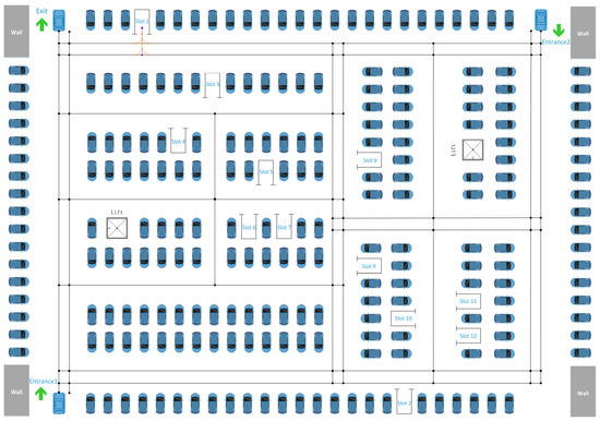
Figure 1.
The underground city parking lot with 234 parking slots can be used to plan the movement and parking of vehicles through a guidance system.
The purpose of the guidance is to allocate acceptable parking slots and plan routes for the cars that will be parked there, which calls for effective planning algorithms to reduce the cost of the parking system’s guidance as well as the operating costs and power consumption of the vehicles.
2.1. Basic Assumptions and Conditions
Figure 1’s parking lot shows two elevator compartments, Entrance 1 at the bottom left, Entrance 2 at the top right, and an exit at the top left. After applying for parking assistance, the motorist moves his vehicle to the entrance and out of the parking space. Following these presumptions, the guidance system was installed in the parking lot:
(1) Guidance applications are issued simultaneously by several vehicles in a short amount of time;
(2) On the road, the vehicles are traveling in either a single-lane or double-lane bidirectional mode. In other words, there are two routes by which the road segment can be passed;
(3) The average speed and straight-line speed of all cars are Vs = 3 m/s;
(4) In the parking lot, cars turn in the same direction and at the same pace;
(5) Assigned vehicles adhere to the guidance program for parking; assigned vehicles are not permitted to access unassigned or other entrances, or to access other slots for parking;
2.2. Guidance System Architecture
The architecture of the parking guidance system primarily consists of planning the optimal route and resolving conflicts between vehicles when parking. In Figure 2, the flow is demonstrated.

Figure 2.
The architecture of the urban parking guidance system.
- Parking slots allocation: The scheduling algorithm takes into account the stopping and waiting time, time through a straight line, turning time, and traffic time of the vehicles, starting from the least time-consuming of all tasks in the entire guided time period of the parking system. Each vehicle’s ideal target position is defined.
- Path planning: The bottom layer algorithm carries out global path planning for each vehicle by taking into account the driving cost and power consumption of the vehicle in-depth, based on the optimal depot position determined by the scheduling algorithm.
- Path conflict resolution: The upper-layer algorithm finally creates a collision-free path for the multi-intelligent vehicle system by resolving the underlying path conflict problem within the CBS framework. The planning of operating pathways requires less computation and time while maintaining the safety of vehicle trajectories.
2.3. Factors Influencing the Allocation of Parking Slots
This section outlines the model’s inputs and discusses the variables that affect parking slot allocation. The parking lot plan in Figure 1 serves as an illustration of the parking lot modeling procedure. The parking lot has 238 slots, each of which is 3 m wide and has m = 12 valid parking slots (Slots 1 through 12). At the node, the vehicle’s turning trajectory is 4.7 m. The reverse parking trajectory is approximately a quarter-circle with radius Ls1 = 1.5 m when the car approaches the front of the parking place. The r1 = 0.5 means that the parking speed when turning is 0.5 times the parking speed when going straight, while parking in reverse is done at a speed equal to straight line travel speed r2 = 0.3 times.
When building the parking spot allocation model, the key influencing aspects should be taken into full consideration [28,29,30]. It is ascertained through the analysis of pertinent studies that the straight line time, the number of curves, the parking situation on both sides of the effective parking slot, and the duration of the shade are the factors taken into consideration by the guidance system for the allocation of parking slots. The ability of intelligent cars to realize autonomous valet parking has increased thanks to advancements in science and technology. By relying on their own high-precision sensors and the cloud scheduling of intelligent parking lots, these vehicles can park themselves more successfully and with less difficulty than they could manually. As a result, the selection of a parking spot is not influenced by the parking conditions on either side of the parking slot. Currently, underground parking is the norm in order to maximize the use of available space and protect automobiles from the sun’s rays. This research identifies four primary factors for parking spot distribution by combining the aforementioned criteria:
1. Straight time: The uniform speed Vs of the road segment is used as the basis for the calculation to guide vehicle i (i = 1, 2,..., n) to park in slot m (m = 1, 2,..., j), the straight time Ts,i of vehicle i is
where the length of the kth section affects coefficient δk. When Lk ≥ 35 m, δk = 1.25; Lk ≤ 12 m, δk = 0.7, and δk = 1 in the remaining road portion. When driving on a longer, two-lane, two-way road, where driving is safer, it may be reasonable to increase the speed of the vehicle. In practice, thorough analysis of the safety of vehicle driving allows the speed of the vehicle to be adjusted according to the condition of the road. When traveling on a single-lane, two-way road, the vehicle’s speed can be suitably adjusted to make room for maneuvering and to prevent collisions. The average driving static speed Vs, or δk = 1, is the speed in the majority of occurrences. Lk also specifies the length of the kth segment.
2. Number of turns: The complexity and smoothness of the intended path are both impacted by the number of turns. The turning time of vehicle i (i = 1, 2,..., n) equals
where x is the number of turns the vehicle must make from the parking lot’s entrance to reach the designated slot. γi,m is a Boolean variable, γi,m = {0,1}, if γi,m = 1, then vehicle i goes through at least one turn, if γi,m = 0, then there are no turns, and ti,k is the time needed for a vehicle to go through a turn. t is the additional utility factor for a single curve, t >1.
3. Traffic time: The current vehicle should instantly implement stop-and-wait procedures, waiting until the vehicle in front of it is entirely parked in the parking slot before continuing to drive. This is critical to stop a collision and subsequently affects the system’s safety. Figure 3 portrays the two phases of the trajectory of reversing into the parking slot: the round trajectory in front of the parking slot (black dashed line) and the straight route inside the parking area (red dashed line).
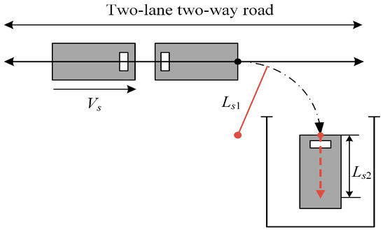
Figure 3.
Diagram of UGVs reversing into the parking slot.
Ls1 is the turning trajectory’s approximate circle radius. The last entry’s Ls2 distance is measured in a straight line. The weight of the vehicle trajectories in these two phases and the time Ta,i required to reverse into the parking slot can be determined using the preceding figure and the presumptions:
The time spent in traffic includes the time needed to back into parking slot Ta,i. Additionally, this time is used up as the current car pulls into its designated parking area.
4. Stop-and-wait time: The guided automobiles in the parking lot must all come to a stop and wait at the entry according to their respective vehicle serial numbers before the scheduling task can officially begin. The vehicle stop-and-wait time Tw has a set value of 8 s because each vehicle and each task has the same function and the time is short.
Vehicles requesting parking are given R tasks by the parking guidance system, and each task’s completion time takes into account the straight, turn, traffic, and stop-and-wait times. From Equations (1)–(5), the completion time Tir for the execution of the r-th (r = 1, 2, …, k) task by the i-th (i = 1, 2, …, n) vehicle is:
The consumed time cost of the system guiding all vehicles to complete the task is:
2.4. Problem Model
The following optimization formulation is the multi-intelligent vehicle scheduling problem in a multi-entry high-density parking lot parking situation:
Building the scheduling model must take the time cost of the parking lot and the multi-intelligent vehicle system into account to ensure the efficient functioning of the parking system [31,32]. As a result, we created Equation (8) with the objective function of the shortest amount of time needed to finish every activity over the entire parking system-guided time period. Equation (9), where R is the total number of tasks, states that each legitimate task in the task list must be carried out. There can only be one vehicle allocated to each task, according to constraint (10). The safety of the multi-intelligent vehicle system’s operation is ensured by constraint (11), which guarantees the system’s collision-free motion, where C is the anticipated number of collisions when the vehicle completes the task. Equation (12) limits the number of vehicles that can park in a parking slot to only one. Equation (13) shows that neither the total number of allotted parking slots nor the total number of vehicles that must be parked exceeds the number of all legally available unoccupied spots in the parking lot. Constraint (14) assures that the amount of time needed for each vehicle to finish this work does not go beyond the amount of time in which the vehicle’s current power can finish it, represented by Er.
3. IACA–IA Based Task Scheduling Algorithm
The objective of scheduling for the parking system is to guarantee the parking lot’s operational effectiveness while taking into account both its operating cost and time cost. For drivers, scheduling entails ensuring parking dependability, avoiding the repetitive parking search phenomenon of conventional parking methods, achieving safety standards while lowering driving costs, minimizing the variance of driving costs for each vehicle, and putting the balance and rationality of the scheduling algorithm into action.
3.1. Application of Conventional Scheduling Algorithms
3.1.1. FCFS Method
One of the most common scheduling methods is First Come First Served (FCFS). When processing tasks, FCFS will process the first-ready tasks in a certain order, with the second-ready tasks being placed at the end of the ready queue. The system will then schedule the tasks according to the order in which the tasks were received. When the FCFS algorithm is utilized for parking lot scheduling, the vehicle that arrives at the parking lot first has a higher parking priority and will enter the lot first to find a parking slot. Because there are no parking guiding instructions, the parker can only wander around the parking lot to find a parking slot. When the vehicle arrives at the parking slot, it must determine whether the space is occupied, before driving away if it is. Although the FCFS method is straightforward to use, the planning outcome lacks scientific rationale.
3.1.2. NACA
The normal ant colony algorithm (NACA) is a swarm intelligence algorithm that mimics how ants search for a path when foraging. The route is chosen based on the pheromones that foraging ants leave behind. The quantity of pheromones released by passing ants is proportional to the number of ants passing through a path, and the likelihood that ants will choose a path is proportional to the strength of the pheromones on the path, creating a positive feedback mechanism that eventually helps ants find a path. The traveler problem, which necessitates balancing the relationships between each city and the beginning and terminating places, is comparable to how NACA tackles the vehicle scheduling problem.
The state transfer probability formula for the NACA core is as follows:
where Pijk is the likelihood that an ant will move from position i to position j. The next choice of position for ant k is indicated by allowedk = {0, 1, …, n − 1} − tabuk. The estimated number of ants traveling from position i to position j is indicated by the expectation heuristic factor ηij.
Although NACA’s solution performance is more robust, its convergence speed is slow. Additionally, because of the presence of a positive feedback mechanism, the gap between the pheromones on each path widens as the number of iterations rises, so the solution that is ultimately produced may not be the best one.
3.2. Improved Ant Colony Scheduling Algorithm
Although NACA can address the assignment results, the solution results are typically poor when utilized to handle the vehicle scheduling problem in a parking scenario. The planning results of NACA are unable to properly account for the prior features of vehicle travel. The main issues with adopting NACA for scheduling are its slow convergence speed, ease of entering local optima, and inadequate scenario adaption.
In the NACA method, the starting values remain constant, and the choice of the subsequent node mostly depends on the desired heuristic factor. The algorithm’s initial stage has inadequate randomization, and it takes longer for positive feedback to start working. As a result, the algorithm’s initial stage convergence is slow. If the initial substandard solution prevails, stronger pheromones will draw in more ants and direct the entire system to evolve in that direction, causing the algorithm to enter a local optimum. Compared to other classic algorithms, NACA finds it more problematic to exit the suboptimal solution.
This work suggests an improved ant colony algorithm (IACA) with higher search randomness, faster convergence, and greater suitability for parking scheduling scenarios in order to address the aforementioned issues. This paper primarily uses the following three optimization techniques: (1) modifying the algorithm’s initial search strategy for the next place; (2) using the expectation factor to increase the path selection’s priority; and (3) using a novel pheromone compression technique.
3.2.1. Chaos Search Strategy
The two phases of the NACA process are typically referred to as the adaption phase and the collaboration phase. The diversity of the adaptation phase is largely what determines whether the optimal solution can be produced in the collaboration phase, making the adaptation phase of NACA more significant. During the adaptation phase, each candidate solution continuously modifies its own structure in response to the information that has accumulated. As a result, during the adaptation phase, we should make the algorithm accept as many different types of search strategies as we can, ensuring that the diverse strategies almost entirely cover the viable domain. We use the chaotic sequence produced by the chaotic mapping to replace the pseudo-random number sequence and use the chaotic sequence to serve as the foundation for the ant colony’s selection of the next vehicle position, thereby increasing the diversity of the algorithm’s search. This is done in accordance with the randomness, ergodicity, and long-term unpredictability of chaotic mapping. This approach typically produces better outcomes than using pseudo-random numbers.
We choose the more common Circle mapping:
where a = 0.5 and b = 2.2. The system denoted by Equation (16) is in a state of complete chaos.
The chaotic search strategy for the next parking slot j is shown in Table 1.

Table 1.
Pseudocode of chaotic search.
Where Nk+1 is the number of unoccupied slots and Zk+1 is the chaotic variable. The next place is chosen using a chaotic search method to increase the algorithm’s ability to perform a global search when a random integer is less than the chaotic perturbation probability Pz. When this random number is greater than or equal to Pz, it enters the non-chaotic search state. When it is lower than another random number, h1, it searches according to the likelihood of pheromone strength. The next place is chosen using a roulette search when this random integer is bigger than or equal to h1. Additionally, the following technique is used to control the range of h1.
where q is the algorithm’s iteration count. This increases the likelihood that probabilistic search techniques will be used during the algorithm’s adaptation phase in the unaltered state to hasten convergence. To enhance the algorithm’s ability to explore, increase the likelihood of the roulette wheel selecting the next slot during the collaboration phase.
3.2.2. Calculation of the Expectation Heuristic Factor
While NACA can address many issues in various contexts, its adaptability and generality depend largely on the application circumstance. Our goal for the vehicle scheduling issue is that it always arrives at the target site in the shortest amount of time and at the lowest possible cost. The state transfer probability Pijk of NACA’s predicted heuristic factor ηij often takes the inverse of the distance between positions i and j, indicating that the likelihood of picking a path with a shorter length is higher. In addition to the distance traveled by the vehicle, the number of turns is another evaluation metric to be taken into account. As a result, we relate the number of turns a vehicle makes along a certain route to the expected heuristic factor:
where c and d are the normalized coefficients. The implementation of the turn count is intended to reduce the number of turns that cars take, or, in the case of two driving-cost-equivalent routes, to increase the visibility of the route with fewer turns. Second, it avoids sudden curves at high speeds, especially when two vehicles are simultaneously turning on a two-lane, two-way road, to prevent crashes that can endanger the vehicle’s safety while it is operating. This change enhances the algorithm’s performance.
3.2.3. Pheromone Compression Strategy
In order to prevent the algorithm from searching only certain pheromone maximum-paths at later stages, or not searching certain smaller pheromone paths, the pheromone will be updated globally when the algorithm completes each cycle. This is done to prevent the gap between pheromones on each path growing wider and wider due to the positive feedback mechanism as the number of iterations increases. This study employs Equation (19) to condense the updated ant pheromones following each generation of a global update:
where σ0 is the beginning value of pheromone concentration, σmax(t) is the maximum pheromone concentration of this iteration, σmin(t) is the minimum pheromone concentration of this iteration, and σ0 + σij(t) can be extended as the pheromone in its path grows, making the compression effect more apparent. The goal of the pheromone compression strategy in this paper is to decrease the pheromone gap of each path, to give the next generation of ants a better chance to find the best solution, to enhance the algorithm’s ability to perform global optimization, and to avoid falling into the local optimal solution too soon.
3.3. IACA–IA Algorithm
There are two heuristic elements in Pijk. The heuristic pheromone factor α, or relative relevance of pheromones gathered by ants during movement in guiding the colony’s search, measures the degree of influence of pheromones on whether the current path is chosen. The strength of the role played by a priori and deterministic factors in the ant colony’s search for the best path can be seen in the magnitude of the expectation heuristic factor β, which represents the guiding nature of the pheromone on the path, guiding the ants to choose the path during the search. The degree of pheromone evaporation is also indicated by the pheromone evaporation coefficient ρ. When the value of ρ is too large, the pheromone evaporation on the path is excessive, which affects the effect of the positive feedback mechanism, and when the value of ρ is too small, the probability of previously searched paths being searched again skyrockets, which affects the algorithm’s ability to perform global searches.
NACA differs from other typical optimization methods in that it performs best when the right parameters are used. The parameters of heuristic components are typically chosen only based on empirical values; however, when the NACA is applied to various circumstances, the values of α, β, and ρ are plainly not invariant, necessitating considerable time and expense to experiment with the best parameter combinations. While the IA can eventually find the global optimal solution even if it starts with a population of subpar solutions, it does not place as much emphasis on the parameters of the algorithm or the quality of the initial solution.
We propose an IACA–IA algorithm to pre-solve the ideal set of parameters for IACA in the parking scheduling situation in order to overcome the aforementioned issues. This gives the algorithm improved convergence and flexibility. The incentive degree of each group of antibodies is calculated using the time required to complete one iteration of each ant colony algorithm and the induced cost T of this parking system.
The pseudocode of IACA–IA is shown in Table 2, where Gimu and Gant are the number of iterations of IA and IACA, respectively.
Table 2.
Pseudocode of IACA–IA.
4. ICBS-Based Multi-Intelligent Vehicle Planning Method
After IACA–IA resolves the slot allocation outcome, a reasonable planning strategy is also required. The movement mode of a single intelligent vehicle may be influenced by other vehicles due to the lack of a global picture of the multi-intelligent vehicle system, contributing to coordination issues and, in extreme circumstances, collision incidents. Multiple intelligent vehicles need to coordinate their planning, which emphasizes the significance of the path-planning algorithm and the conflict removal method. We adopt a central scheduling structure in a high-density parking lot, and the scheduling host will perform all of the planning calculations.
In this work, the planning of numerous intelligent vehicles is carried out using the CBS algorithm with a two-tier framework structure. Separate analyses and improvements are made to the two frameworks’ computational approaches. For the initial path planning of vehicles, we adopt a straightforward implementation of the A* algorithm at the bottom layer. We then propose an enhanced heuristic function-based adaptive dynamic A* algorithm (ADA*), which addresses the issue of the standard A* algorithm’s lengthy computation time [33]. For constraining tree nodes, the upper method introduces a bi-objective expansion mechanism. The performance of the method and its computational aspect are both improved by simultaneously considering the two phases mentioned above in the same framework in this paper.
4.1. ADA* Heuristic Function Optimization
The A* algorithm is a path-finding and map traversal algorithm with high accuracy. G(n) is the result we can accurately deduce from the calculation and H(n) is a heuristic function that approximates a value. The core of its search is to approximate the target point using the combined priority F(n) of nodes.
The A* algorithm’s search efficiency depends on the heuristic function. Particularly in the high-density parking lot scenario, where the map is more complicated, this might result in a significant accumulation of erroneous traversal nodes because the estimate of H(n) is always smaller than its true value, lowering the search efficiency. The algorithm can locate the shortest path and the search speed is quick if we can make the estimate of H(n) infinitely near to the true value. Because of this, Zhao et al. [19] weighted H(n) and came up with the following integrated priority:
where m is the weight coefficient. After the weighting process, the algorithm’s performance is enhanced. However, when the process iterates, the subsequent stages should gradually see the current node approach the target point, the size of H(n) approach the accurate amount, and the ratio of the weights m to the weights of G(n) approach 1:1. Evidently, using constant weights does not accommodate the entire algorithm traversal procedure. We enhance this foundation and utilize the adaptive concept from control theory to modifying the heuristic function to solve the aforementioned issues.
Equation (21) can make sure that the first search’s H-value can be adjusted to make it infinitely close to the real consumption value. The adaptive weight progressively becomes closer to 1 as the distance between the current node and the target point decreases. The algorithm’s traversal approach is fundamentally improved by ADA*, which also significantly speeds up the algorithm’s search time and decreases the amount of time needed for path planning.
4.2. Updating the Extended Model
With the planning scheme obtained by the underlying algorithm ADA*, the upper layer algorithm constructs a constraint tree with a binary tree structure. It then performs online conflict detection and adds constraints to the constraint tree to resolve conflicts (the constraint element information {ai, n, t1} indicates that the vehicle ai is prohibited from occupying node at moment t1), then calls ADA* once more to plan the vehicle paths that adhere to the constraints until it reaches the parking slot. The UGV system is rather large in this framework, and the ADA* is linearly related to the map scale. The planning method will result in a significant number of nodes inside the constraint tree expanding as more vehicles enter the parking lot. The normal constraint tree, on the other hand, is enlarged by a single cost function, resulting in several erroneous expansion amounts in numerous similar cost functions, repeatedly calling the underlying algorithm and substantially impairing planning efficiency.
A specific planning case is provided in Figure 4 below. In this study, the unweighted undirected graph for the problem of many intelligent vehicles planning their paths is built using a two-dimensional four-neighborhood raster map. Assume that Figure 4 depicts a specific area in a parking lot; yellow dots denote slots that have previously been occupied by other vehicles; and that there are three UGVs—a1, a2, and a3—in the parking lot. The starting positions, target positions, and initial planning paths of each of these vehicles are also shown.
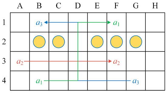
Figure 4.
The planning case uses the extended model of this paper. The starting points of UGVs a1, a2, and a3 are B4, A3, and G4, respectively, and the target points are F1, F3, and B1, respectively.
The unfolding partial constraint tree structure is depicted in Figure 5 if the normal constraint tree is enlarged in a single-objective way using the multi-intelligent vehicle system’s path cost as the objective function. The conflict position D3 at the root node R is discovered using the higher-level algorithm. R divides into two nodes for the constraint tree, R1 and R2, and two sets of conflict meta-information, {a1, D3, 3}, and {a2, D3, 3}, respectively. The goal function has the same cost of both 21 and the path conflict is identified again in R1 and R2, so the system cannot reasonably judge the node’s quality. As a result, this situation will continue to divide for numerous sub-nodes, R3, R4, R5, and R6, to carry out a conflict search once again.
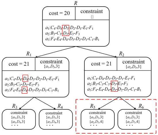
Figure 5.
Constraint tree extension model.
For the aforementioned issues, we build a dual-objective extension model with the best single-vehicle driving characteristics as the second layer objective and the path cost minimization of the multi-intelligent vehicle system as the first layer objective. Specifically, the first layer objective function is removed when the upper layer algorithm detects a path conflict if the total path cost is the same at the same level of the constraint tree, and the best solution is chosen by carefully taking into account the optimum driving features of a single vehicle. We define the optimum driving features of the vehicle as its power consumption and the shortest time to complete a task in order to highlight the differences. In the parking lot, there are three different driving styles, and each one has a different power consumption. We define the power consumption of the vehicle in the waiting state at 0.3 and the power consumption in the non-waiting (straight ahead, turning) state as 1, in order to guide the vehicle to reach the target point with the lowest possible cost. A new function is created by these parameters and the multi-intelligent vehicle system’s path cost:
In the formula:
ZRn is the combined priority of the second-level objective function of the Rnth constraint tree node. CRn is the total path cost of the Rnth constraint tree node. Tir and Eir are the time to perform task r of smart vehicle i, the least time-consuming of the Rnth constraint tree node, and the power consumption of smart vehicle i to perform task r, respectively. A smart vehicle is supposed to run a cell raster normally in one unit of time. We use the ratio of the sum of the two to the total path cost as a reference basis and add it to the total path cost to form the optimum driving characteristics for each smart vehicle, since there is only a slight difference between power consumption and task completion time for each smart vehicle after extensive calculations.
The method is used to once more deconflict the case of Figure 4’s beginning path. Figure 5 shows that the total path cost in the R1 and R2 constraint tree nodes is the same, indicating that the expansion strategy’s first layer of the objective function is also the same. We discover that, for the vehicle a2 in R1 after five units of time, the task completion time is the shortest, consistent with the judgment condition, and its operating duration and power consumption are 5. This is consistent with the idea of the dual-objective expansion model. ZR1 is 21.47 when we add the complete path cost of R1 to it. Vehicle a2 in R2 meets the judging criteria with a minimal task completion time of one wait and five units of straight travel, and its operating time and power consumption are 6 and 5.3, respectively. ZR2 is 21.54 when added to the overall path cost of R2. In order to continue the expansion and discard the children nodes of the R2 branch, the constraint elements are formed in accordance with conflicts in the planning scheme of node R1, which is computed to be more consistent with the expansion model (red dashed line). The expansion strategy with dual objectives has fewer nodes in the constraint tree, and the number of calls to the underlying algorithm is reduced from seven to five. As a result, the complexity of the constraint tree and the computation of the algorithm are both significantly reduced, especially in the complex environment of multi-vehicle systems, leading to a significant simplification effect.
The objective is to fully take into account the optimum driving features of each individual vehicle in addition to achieving the best multiple UGV systems. In a high-density parking environment with dense vehicles and narrow paths, we want a single vehicle to finish parking as soon as possible to minimize the impact on other vehicles and avoid generating more path conflicts, which makes the constraint tree more complex and therefore generates many invalid computation volumes. This is especially true when multiple vehicles are driving in a single-lane, two-way roadway at the same time. This model achieves the expanded purpose of lowering the system cost and maximizing the driving features of a single vehicle while overcoming the limitations of the single-objective model solution.
5. Simulation Verification
In order to solve the vehicle scheduling problem of simultaneous application for parking induction at different entrances of high-density parking lots, we combine a task scheduling algorithm, path planning, and conflict resolution algorithm in this section. We also design three traditional scenarios for simulation experiments. In addition to evaluating and analyzing the FCFS, NACA, and IA algorithms with the proposed IACA–IA scheduling algorithm, we also compare and contrast the ICBS and CBS algorithms.
5.1. Simulation Setup
All of the simulation tests in this section were performed on a computer with an Intel Core i9-10900 processor clocked at 2.80 GHz and 32 GB of RAM in environment matlab2021a. This study assumes that a single vehicle can occupy exactly one raster vertex and that a vehicle uses a one-time unit for each cell raster vertex during normal operation to create a two-dimensional, four-neighborhood raster map of the parking environment. The key parameters of the algorithm were set as follows:
m = 50, Pc = 0.8, Pm = 0.1, Pz = 0.06, Q0 = 45, Qi = 1, h1 = 1, Np = 120, Nc = 0.5, Gimu = 300, Gant = 800.
5.2. Analysis of IACA–IA Scheduling Algorithm
5.2.1. Scenario 1
Using Entrance 1 and Entrance 2, Scenario 1 (see Supplementary Materials) implements a load-balancing strategy. There are six vehicles at each entry, which is the same as the number of vehicles requesting parking guidance at Entrances 1 and 2. There are still 12 valid parking slots available in the parking lot, marked slots 1 through 12, and the vehicles that need to be parked stop at the entry in the order of their serial numbers and wait for the guidance system’s scheduling instructions.
Selection of Parameter Combinations
The training results of the IACA–IA algorithm were passed 300 times in matlab2021a, as shown in Table 3, and we selected the top 20 antibody sets in terms of incentive degree. The above antibody sets represent various combinations of the three parameters of the IACA pheromone heuristic factor α, expectation heuristic factor β, and pheromone evaporation coefficient ρ under the parking scenario in this paper.
Table 3.
The set of antibodies with the top 20 incentive degrees was taken as the IACA–IA simulation results.
According to Table 3, the parameter combination {α = 5.288, β = 6.865, ρ = 0.293} of the suboptimal solution has an incentive of 0.214, but the lowest one has one of 0.073, which is an almost threefold difference. In order to improve the scheduling algorithm’s ability to adapt to the scenario in this study, we select the best solution {α = 2.927, β = 4.308, ρ = 0.278} as the parameter combination for the IACA.
Simulation Results
We first assigned parking slots to 12 vehicles based on the optimal scheduling algorithm and then performed an extensive comparison with other algorithms from distinct viewpoints.
In the parking lot simulation for Scenario 1, shown in Figure 6, each vehicle is queued up at the entrance according to its serial number (vehicles 1 to 6 from top to bottom at Entrance 1, and vehicles 7 to 12 from bottom to top at Entrance 2).
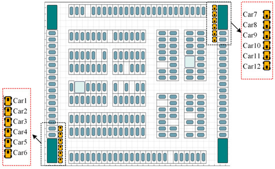
Figure 6.
Scenario 1 simulation.
The parking slot assignment result graph, which is depicted in Figure 7, reflects the scheduling outcome for each vehicle using the algorithm presented in this research. Figure 8 displays the induced costs for each vehicle using the FCFS, IA, NACA, and IACA algorithms. Figure 9 shows the costs for the three algorithms IA, NACA, and IACA after 800 iterations.

Figure 7.
Parking allocation results in Scenario 1.

Figure 8.
Parking cost for each vehicle in Scenario 1.
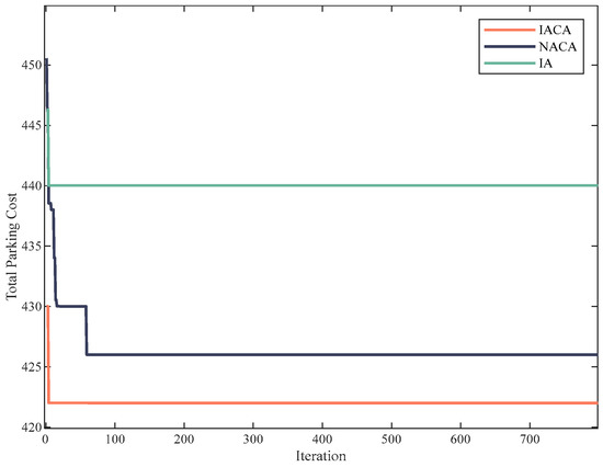
Figure 9.
Algorithm iteration result in Scenario 1.
Analysis of Results
The aforementioned experimental results show that a variety of algorithms can address these problems, but there is a big variation in how effective the solutions are. When using the FCFS method, the order of task generation is determined by the order in which the vehicles enter the parking lot. Utilizing FCFS, the parking system’s total guided cost is 486.2 while using IACA, the scheduling task’s total guided cost is 422. The cost sought by the algorithm in this work is 13.2% lower than the cost sought by the FCFS method, the cost per vehicle is more average, and the difference between the maximum cost and the minimum cost is no greater than 6. However, utilizing the FCFS method results in higher costs overall, as well as more differences in costs per vehicle. As an illustration, the cost of Vehicle 7 through Entrance 2 and Vehicle 12 from the same entrance is 15.3 and 73.9, respectively, which as almost five-fold difference.
IA and IACA both have high convergence abilities, as demonstrated in Figure 9, and both methods may converge in fewer than 10 iterations. However, the solution found by IA is not ideal and costs 440, whereas the optimal solution obtained by the approach in this study is 422. After 66 iterations, NACA achieves a cost of 426, which is higher than the approach presented in this study but lower than IA, and was slightly slower to converge.
5.2.2. Scenario 2
Using Entrance 1 and Entrance 2, Scenario 2 (see Supplementary Materials) implements a load-unbalancing strategy. The number of vehicles requesting parking guidance at Entrances 1 and 2 differs and is less than the number of available spaces; Entrance 1 has two vehicles, and Entrance 2 has seven vehicles. There are still 12 valid parking slots available in the parking lot, marked slots 1 through 12, and the vehicles that need to be parked stop at the entrance in the order of their serial numbers and wait for the guidance system’s scheduling instructions.
Simulation Results
We first assigned parking slots to nine vehicles based on the optimal scheduling algorithm and then performed an extensive comparison with other algorithms from distinct viewpoints.
In the parking lot simulation for Scenario 2, shown in Figure 10, each vehicle is queued up at the entrance according to its serial number (Vehicles 1 to 2 from top to bottom at Entrance 1, and Vehicles 3 to 9 from bottom to top at Entrance 2).

Figure 10.
Scenario 2 simulation.
The parking slot assignment result graph, which is depicted in Figure 11, reflects the scheduling outcome for each vehicle using the algorithm presented in this research. Figure 12 displays the induced costs for each vehicle using the FCFS, IA, NACA, and IACA algorithms. Figure 13 shows the costs for the three algorithms—IA, NACA, and IACA—after 800 iterations.
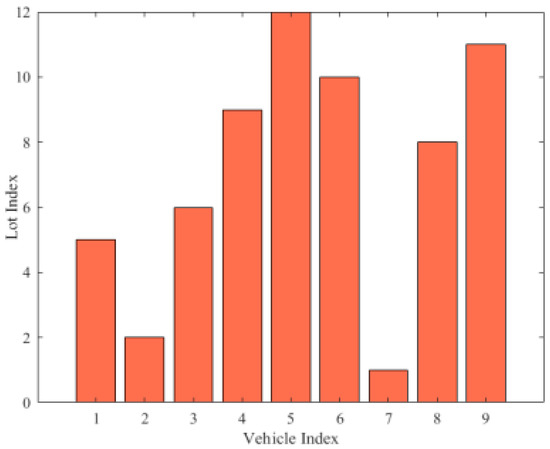
Figure 11.
Parking allocation results in Scenario 2.

Figure 12.
Parking cost for each vehicle in Scenario 2.
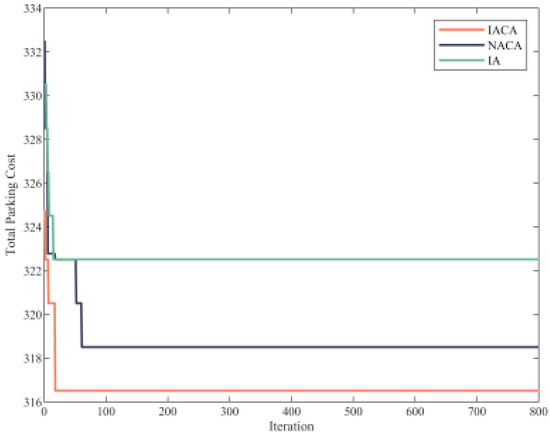
Figure 13.
Algorithm iteration result in Scenario 2.
Analysis of Results
The aforementioned experimental results show that a variety of algorithms can address the problems, but there is a big variation in how effective the solutions are. When using the FCFS method, the order of task generation is determined by the order in which the vehicles enter the parking lot. Utilizing FCFS, the parking system’s total guided cost is 360.4, while using IACA, the scheduling task’s total guided cost is 316.4. The cost sought by the algorithm in this work is 12.2% lower than the cost sought by the FCFS method, the cost per vehicle is more average, and the difference between the maximum cost and the minimum cost is no greater than 8. However, utilizing the FCFS method results in higher costs overall, as well as a greater difference in cost per vehicle. As an illustration, the cost of Vehicle 8 from Entrance 2 and Vehicle 7 from the same entrance is 14.6 and 57.3, respectively, a nearly four-fold difference.
IA and IACA both have high convergence abilities, as demonstrated in Figure 13, and both methods may converge in fewer than 20 iterations. However, the solution found by IA is not ideal and costs 322.4, whereas the optimal solution obtained by the approach in this study is 316.3. After 64 iterations, NACA achieves a cost of 318.3, which is higher than the approach presented in this study but lower than IA and slightly slower to converge.
5.2.3. Scenario 3
Using Entrance 1 and Entrance 2, Scenario 3 (see Supplementary Materials) implements a load-unbalancing strategy. The number of vehicles requesting parking guidance at Entrances 1 and 2 differs and is greater than the number of available spaces; Entrance 1 has six vehicles, and Entrance 2 has 10 vehicles. There are still 12 valid parking slots available in the parking lot, marked slots 1 through 12, and the vehicles that need to be parked stop at the entry in the order of their serial numbers and wait for the guidance system’s scheduling instructions.
Simulation Results
According to the optimum scheduling algorithm, we first identify whether there is a phenomenon that will exceed the parking lot’s capacity, in order to prevent these vehicles from going around in the parking lot and eventually being forced to travel to the next parking lot to find a parking slot because they cannot find a parking slot and then assign the remaining vehicles to the slot, and perform a full comparison analysis with other algorithms.
In the parking lot simulation for Scenario 3, shown in Figure 14. As the number of vehicles to be parked exceeds the number of remaining slots, we only guide 6 vehicles at entrance 2, with all remaining vehicles waiting at the entrance according to their serial numbers (vehicles 1 to 6 from top to bottom at Entrance 1, and vehicles 7 to 12 from bottom to top at Entrance 2).
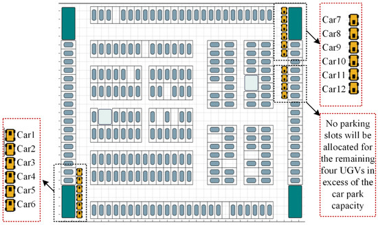
Figure 14.
Scenario 3 simulation diagram.
The parking slot assignment result graph, which is depicted in Figure 15, reflects the scheduling outcome for each vehicle using the algorithm presented in this research. Figure 16 displays the induced costs for each vehicle using the FCFS, IA, NACA, and IACA algorithms. Figure 17 shows the costs for the three algorithms IA, NACA, and IACA after 800 iterations.

Figure 15.
Parking allocation results in Scenario 3.

Figure 16.
Parking cost for each vehicle in Scenario 3.
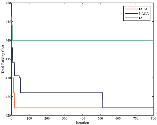
Figure 17.
Algorithm iteration result in Scenario 3.
Analysis of Results
The aforementioned experimental results show that a variety of algorithms can address the problems, but there is a big variation in how effective the solutions are. When using the FCFS method, the order of task generation is determined by the order in which the vehicles enter the parking lot. Due to a lack of parking guiding indications, vehicles 13 through 16 must circle the parking lot in order to find a slot, which not only wastes time and increases useless traffic volume but also makes it difficult to find an acceptable parking slot. Utilizing FCFS, the parking system’s total guided cost is 734.6, while using IACA, the scheduling task’s total guided cost is 422. The cost sought by the algorithm in this work is 42.6% lower than the cost sought by the FCFS method, the cost per vehicle is more average, and the difference between the maximum cost and the minimum cost is no greater than 6. However, utilizing the FCFS method results in higher costs overall as well as a greater difference in cost per vehicle. As an illustration, the cost for Vehicle 7 from Entrance 2 and Vehicle 12 from the same entrance is 15.3 and 73.9, respectively, a nearly five-fold difference.
IA and IACA both have high convergence abilities, as demonstrated in Figure 17, and both methods may converge in fewer than 20 iterations. However, the solution found by IA is not ideal and costs 440, whereas the optimal solution obtained by the approach in this study is 422. The iterative solution speed of NACA is 2585% slower than IACA, and the solution efficiency is unacceptably low, even though it reaches the best answer after 517 iterations.
5.3. ICBS Planning Algorithm Analysis
According to the allocation result of the slot of IACA–IA scheduling algorithm, the planning problem is solved by splitting it into two levels of the ICBS algorithm as a solver, with the bottom layer of the algorithm adopting the ADA* algorithm to solve the path planning problem of multiple intelligent vehicles, and the upper layer adopting the constraint tree expansion strategy of the double objective to optimize the phase conflict and node conflict existing in it, i.e., each intelligent vehicle’s collision-free paths are eventually discovered. The algorithm in this paper will be compared to and evaluated using the TCBS algorithm in order to further validate the solution efficiency and quality of the algorithm.
5.3.1. Scenario 1
Simulation Results
By locating the designated slot point, the ICBS algorithm is used to determine the path of each intelligent vehicle that avoids collisions (Figure 7). Figure 18 displays each vehicle’s route. Figure 19 depicts the route taken by cars at Entrance 1. The movement of vehicles at Entrance 2 is seen in Figure 20. The final experimental results are represented in Table 4 by the average of the experimental data after 100 iterations of each of the TCBS and ICBS algorithms. Figure 21 shows the set of costs solved by TCBS. Figure 22 shows the set of costs solved by ICBS. Figure 23 shows a comparison of the costs of TCBS and ICBS solutions. Figure 24 shows the set of runtimes solved by TCBS. Figure 25 shows the set of runtimes for the ICBS solution. Figure 26 shows a comparison of the runtimes of the TCBS and ICBS solutions. Figure 21, Figure 22, Figure 23, Figure 24, Figure 25 and Figure 26 all present the results of 100 simulation experiments.

Figure 18.
All vehicle paths in Scenario 1.
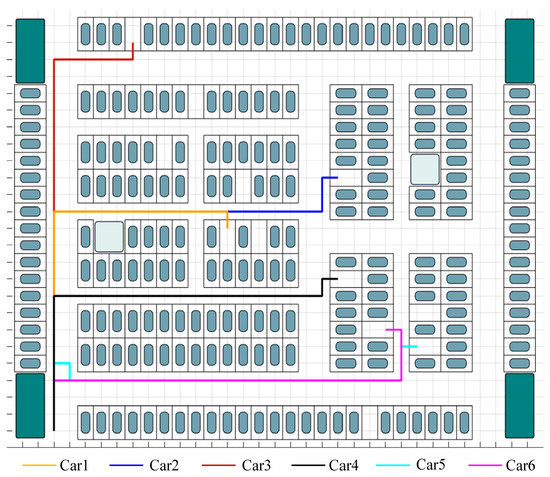
Figure 19.
Entrance 1 vehicle paths in Scenario 1.
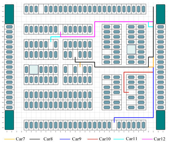
Figure 20.
Entrance 2 vehicle paths in Scenario 1.
Table 4.
Comprehensive comparison between TCBS and ICBS in Scenario 1.

Figure 21.
TCBS cost set in Scenario 1.
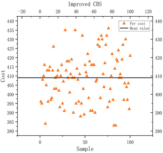
Figure 22.
ICBS cost set in Scenario 1.

Figure 23.
Cost comparison between TCBS and ICBS in Scenario 1.
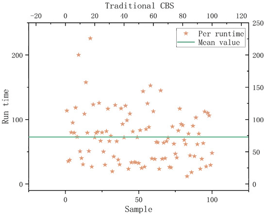
Figure 24.
TCBS run time set in Scenario 1.
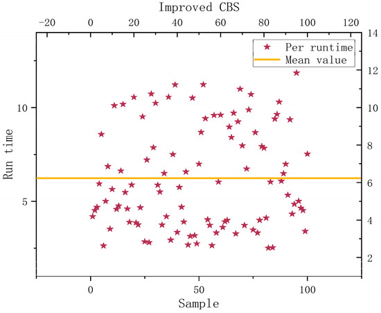
Figure 25.
ICBS run time set in Scenario 1.

Figure 26.
Time comparison between TCBS and ICBS in Scenario 1.
Analysis of Results
The simulation experiments show that, although both algorithms can solve the planning results under parking Scenario 1, the total cost and total energy consumption of vehicles planned by ICBS are 97.92–101.25% of that of the TCBS algorithm in terms of algorithm performance. In terms of algorithm computation, ICBS reduces the solution time by 91.45%, the number of conflict points by 17.73%, and the number of constraint tree nodes by 28.03% compared to the TCBS algorithm. Significant benefits were realized in the test by the improved method. Although ICBS did not considerably lower the cost of the multi-intelligent vehicle system, as shown in Figure 23, it can discover a better planning solution, which TCBS cannot solve, and reduces the number of conflict sites, which is adequate to ensure the vehicle’s safety. When the surroundings are complicated, TCBS takes a lot of time. Due to ADA* and a bi-objective extension model that simultaneously optimizes the upper and lower algorithms, ICBS significantly increases planning effectiveness.
5.3.2. Scenario 2
Simulation Results
By locating the designated slot point, the ICBS algorithm is used to determine a path for each intelligent vehicle that avoids collisions (Figure 11). Figure 27 displays each vehicle’s route. Figure 28 depicts the route taken by cars at Entrance 1. The movement of vehicles at Entrance 2 is seen in Figure 29. The final experimental results are represented in Table 5 by the average of the experimental data after 100 iterations of each of the TCBS and ICBS algorithms. Figure 30 shows the set of costs solved by TCBS. Figure 31 shows the set of costs solved by ICBS. Figure 32 shows a comparison of the costs of TCBS and ICBS solutions. Figure 33 shows the set of runtimes solved by TCBS. Figure 34 shows the set of runtimes for the ICBS solution. Figure 35 shows a comparison of the runtimes of the TCBS and ICBS solutions. Figure 30, Figure 31, Figure 32, Figure 33, Figure 34 and Figure 35 all present the results of 100 simulation experiments.
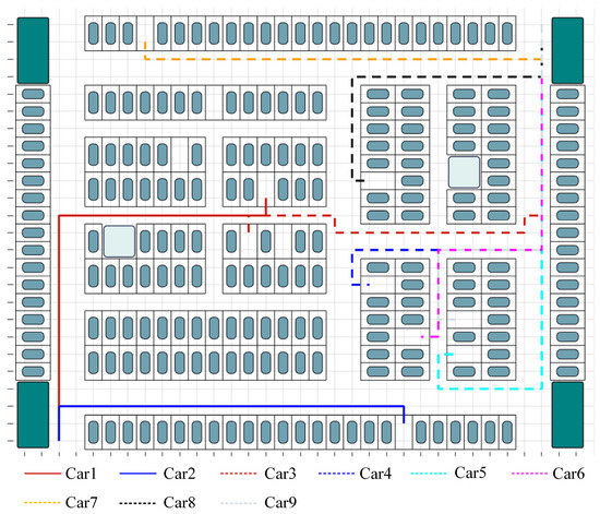
Figure 27.
All vehicle paths in Scenario 2.
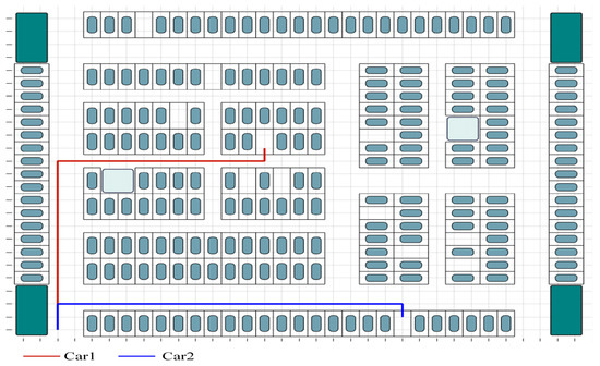
Figure 28.
Entrance 1 vehicle paths in Scenario 2.
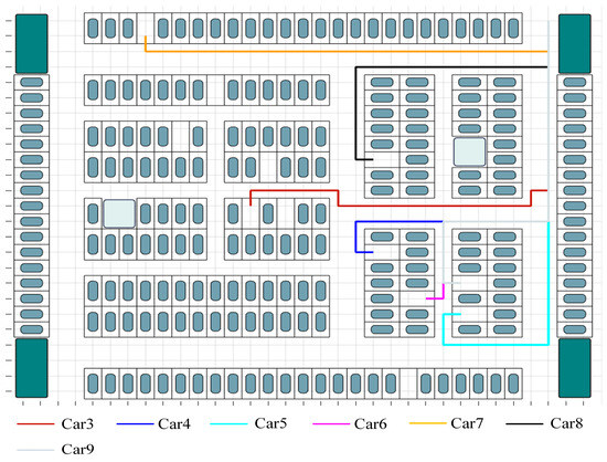
Figure 29.
Entrance 2 vehicle paths in Scenario 2.
Table 5.
Comprehensive comparison between TCBS and ICBS in Scenario 2.
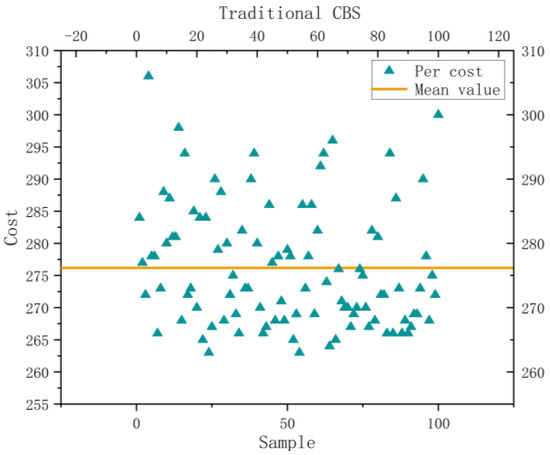
Figure 30.
TCBS cost set in Scenario 2.
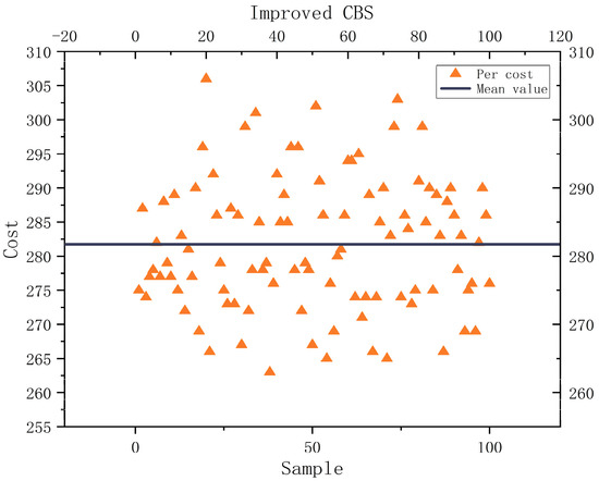
Figure 31.
ICBS cost set in Scenario 2.
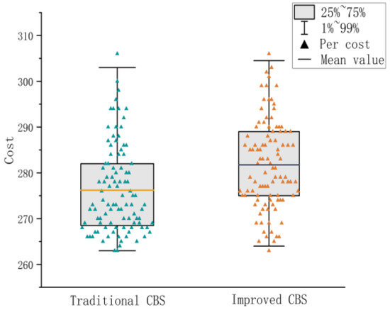
Figure 32.
Cost comparison between TCBS and ICBS in Scenario 2.
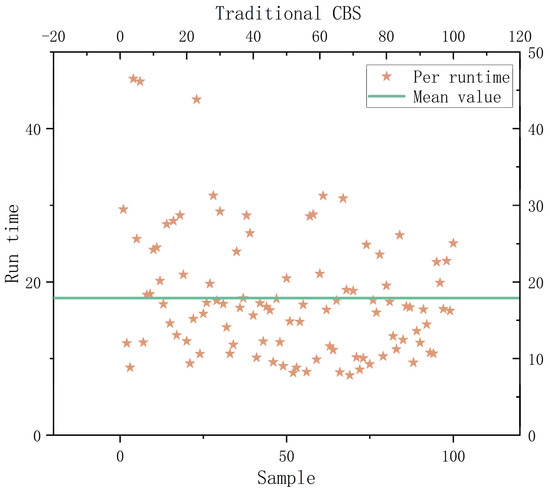
Figure 33.
TCBS run time set in Scenario 2.
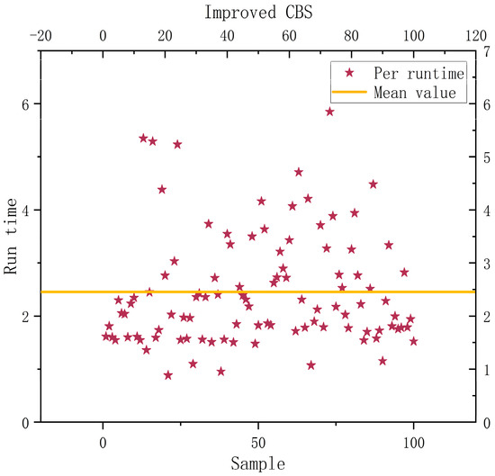
Figure 34.
ICBS run time set in Scenario 2.
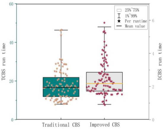
Figure 35.
Time comparison between TCBS and ICBS in Scenario 2.
Analysis of Results
The simulation experiments show that although both algorithms can solve the planning results under the parking Scenario 2, the total cost and total energy consumption of vehicles planned by ICBS are 99.62–102.02% of that of the TCBS algorithm in terms of algorithm performance. In terms of algorithm computation, ICBS reduces the solution time by 86.29%, the number of conflict points by 12.98%, and the number of constraint tree nodes by 24.95% compared to the TCBS algorithm. Significant benefits were realized in the test by the improved method. Although ICBS did not considerably lower the cost of the multi-intelligent vehicle system, it can reduce the number of conflict sites, which is adequate to ensure the vehicle’s safety. When the surroundings are complicated, TCBS takes a lot of time. Due to ADA* and a bi-objective extension model that simultaneously optimizes the upper and lower algorithms, ICBS significantly increases planning effectiveness.
5.3.3. Scenario 3
Simulation Results
By locating the designated slot point, the ICBS algorithm is used to determine the path of each intelligent vehicle that avoids collisions (Figure 15). Figure 36 displays each vehicle’s route. Figure 37 depicts the route taken by cars at Entrance 1. The movement of vehicles at Entrance 2 is seen in Figure 38. The final experimental results are represented in Table 6 by the average of the experimental data after 100 iterations of each of the TCBS and ICBS algorithms. Figure 39 shows the set of costs solved by TCBS. Figure 40 shows the set of costs solved by ICBS. Figure 41 shows a comparison of the costs of TCBS and ICBS solutions. Figure 42 shows the set of runtimes solved by TCBS. Figure 43 shows the set of runtimes for the ICBS solution. Figure 44 shows a comparison of the runtimes of the TCBS and ICBS solutions. Figure 39, Figure 40, Figure 41, Figure 42, Figure 43 and Figure 44 all present the results of 100 simulation experiments.
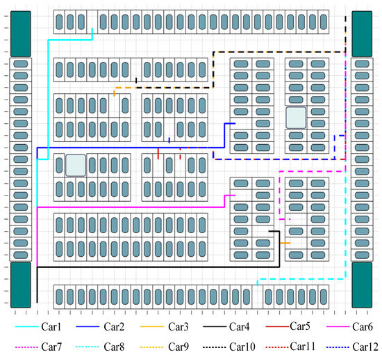
Figure 36.
All vehicle paths in Scenario 3.
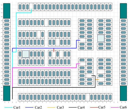
Figure 37.
Entrance 1 vehicle paths in Scenario 3.
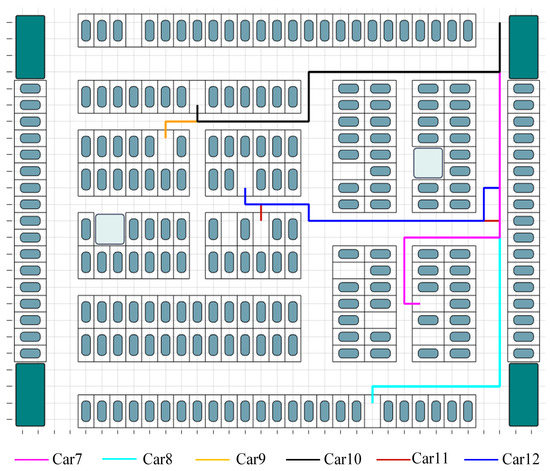
Figure 38.
Entrance 2 vehicle paths in Scenario 3.
Table 6.
Comprehensive comparison between TCBS and ICBS in Scenario 3.
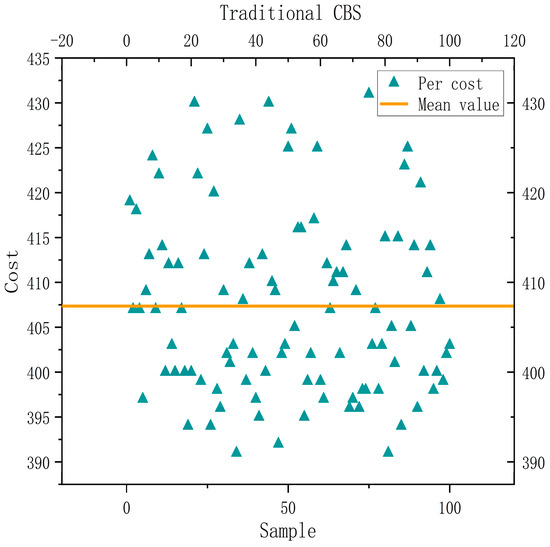
Figure 39.
TCBS cost set in Scenario 3.
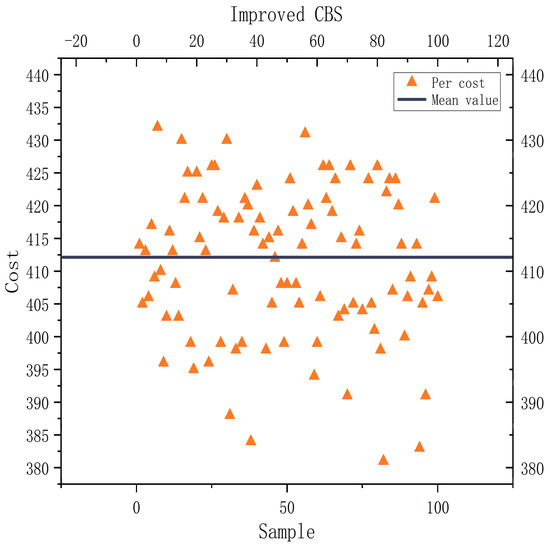
Figure 40.
ICBS cost set in Scenario 3.
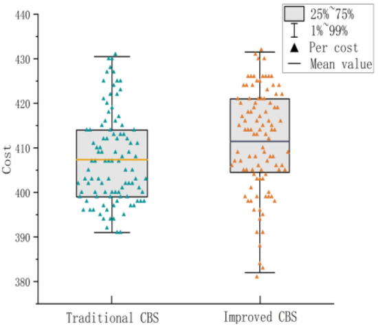
Figure 41.
Cost comparison between TCBS and ICBS in Scenario 3.
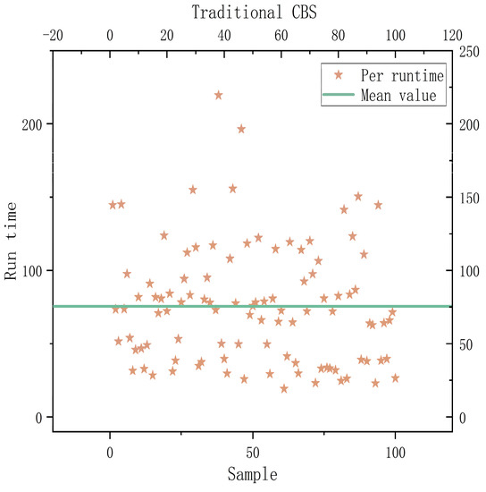
Figure 42.
TCBS run time set in Scenario 3.
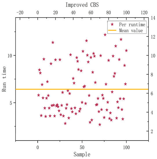
Figure 43.
ICBS run time set in Scenario 3.

Figure 44.
Time comparison between TCBS and ICBS in Scenario 3.
Analysis of Results
The simulation experiments show that although both algorithms can solve the planning results under the parking Scenario 3, the total cost and total energy consumption of vehicles planned by ICBS are 97.44–101.73% of that of TCBS algorithm in terms of algorithm performance. In terms of algorithm computation, ICBS reduces the solution time by 91.48%, the number of conflict points by 10.01%, and the number of constraint tree nodes by 21.45% compared to the TCBS algorithm. Significant benefits were realized in the test by the improved method. Although ICBS did not considerably lower the cost of the multi-intelligent vehicle system, as shown in Figure 41, it can discover a better planning solution that TCBS cannot solve and reduce the number of conflict sites, which is adequate to ensure the vehicle’s safety. When the surroundings are complicated, TCBS takes a lot of time. Due to ADA* and a bi-objective extension model that simultaneously optimizes the upper and lower algorithms, ICBS significantly increases planning effectiveness. As a result, the proposed method in this paper takes less time for planning and improves node redundancy. The aim of simplifying the computational complexity and promoting planning efficiency is achieved with essentially the same total cost.
6. Conclusions
The scheduling of UGVs at different high-density parking lot entrances is researched in this paper, along with parking slot allocation algorithms, path-planning algorithms, and conflict resolution methods. We create a hybrid algorithm to handle the parking slot allocation problem by combining an ant colony algorithm and a diversity of immune algorithms. Additionally, we design an ADA* algorithm as the underlying algorithm to plan vehicle paths and use a dual-objective expansion strategy of constraint trees to efficiently reduce the computational effort of the upper-level methods to solve various types of path conflicts in order to improve the real-time performance of the algorithm. Optimal parking slot allocation avoids the need for repeated slot searches, reasonable path planning lowers the cost of vehicle travel, and conflict resolution in line with this provides safe vehicle travel. When taken as a whole, the planning strategy proposed in this paper increases planning efficiency while assuring safe driving, preventing time and resource waste, and attaining the objective of innovative urban mobility. Further optimization of the planning scheme considering the dynamic scenario of parking lot vehicle entry and exit is a problem that requires further in-depth detail.
Supplementary Materials
The following supporting information can be downloaded at: https://www.mdpi.com/article/10.3390/drones7050295/s1.
Author Contributions
Conceptualization, H.C. and D.Z.; methodology, H.C.; software, H.C.; validation, H.C., Y.Y. and Z.S.; formal analysis, H.C.; investigation, H.C.; resources, Z.D.; data curation, H.C.; writing—original draft preparation, H.C.; writing—review and editing, D.Z.; visualization, Y.H.; supervision, L.X.; project administration, B.L.; funding acquisition, Y.Y. All authors have read and agreed to the published version of the manuscript.
Funding
1. The Science and Technology Research Project of the Education Department of Jiangxi Province in 2021 (Grant No. GJJ210662). 2. the Key Research and Development Project of Jiangxi Province (Grant No. 20224BBE51048). 3. the Start-up Program for Doctoral Research of East China Jiaotong University (Grant No. 579, Grant No. 562). 4. the High-end Foreign Expert Talents Project of Ministry of Science and Technology of China (Grant No. G2021022002L). 5. the National Natural Science Foundation of China (Grant No. 52067006). 6. the High-end Talents Project of Science and Technology Innovation of Jiangxi Province (Grant No. jxsq2019101027).
Data Availability Statement
The data that support the findings of this study are available from the corresponding author, [Yinquan Yu], upon reasonable request.
Acknowledgments
The authors thank the assistance from other people at the School of Mechatronics and Vehicle Engineering, East China Jiaotong University, the School of Automotive Studies, Tongji University and Clean Energy Automotive Engineering Center, Tongji University, College of Mechanical and Electrical Engineering, and the Nanchang Automotive Institution of Intelligence & New Energy.
Conflicts of Interest
The authors declare no conflict of interest.
Abbreviations
| Unmanned Ground Vehicle speed in a straight line. | |
| Number of effective empty parking slots (). | |
| Radius of the approximate circle of the reverse parking trajectory. | |
| Reversing into the slot straight line distance. | |
| Weighting of reversing into parking straight line speed relative to straight line driving. | |
| Vehicle serial number (). | |
| Straight ahead time of vehicles. | |
| Turning time of the vehicles. | |
| Traffic time of vehicles. | |
| Waiting time for vehicles to stop. | |
| Coefficient for adjusting the speed of the vehicle. | |
| Length of segment k. | |
| Number of curves passed by vehicle i. | |
| Additional utility factor for a single turn. | |
| Boolean variables. | |
| Time it takes for a vehicle to go through a curve. | |
| Number of tasks assigned to vehicles by the parking guidance system. | |
| Task serial number of the vehicle (). | |
| Completion time of vehicle i performing task r. | |
| Number of collisions while the vehicle was performing its task. | |
| Time the vehicle can complete its task with the available power. | |
| Probability of ant k moving from position i to position j. | |
| Expectation factor. | |
| Chaotic variable. | |
| Number of remaining parking slots. | |
| Chaotic Perturbation Probability. | |
| Number of IACA iterations. | |
| Maximum pheromone concentration at t iteration. | |
| Minimum pheromone concentration at t iteration. | |
| Beginning value of pheromone concentration. | |
| Pheromone heuristic factors. | |
| Expected heuristic factor. | |
| Pheromone evaporation factor. | |
| Integrated priority of nodes. | |
| Distance from the starting point to the current node. | |
| Estimated distance from the current node to the endpoint. | |
| Combined priority of the second level objective function of the constraint tree node Rn. | |
| Total path cost of a constraint tree node Rn. | |
| Least time-consuming vehicle i in Rn to perform task r. | |
| Power consumption of the least time-consuming vehicle i in Rn to perform task r. |
References
- Liu, Q.; Li, Z.; Yuan, S.; Zhu, Y.; Li, X. Review on Vehicle Detection Technology for Unmanned Ground Vehicles. Sensors 2021, 21, 1354. [Google Scholar] [CrossRef] [PubMed]
- Yang, X.; Jiang, L. Bi-level objective berth allocation model based on the minimum total system time consumption. Univ. Shanghai Sci. Technol. 2021, 43, 179–185. [Google Scholar]
- Zhao, Z.; Zhang, Y.; Shi, J.; Long, L.; Lu, Z. Robust Lidar-Inertial Odometry with Ground Condition Perception and Optimization Algorithm for UGV. Sensors 2022, 22, 7424. [Google Scholar] [CrossRef] [PubMed]
- Ji, Y.; Cheng, F.; Xiao, Z. Research on Optimal Setting of Shared parking Space adjacent to private parking lot in urban center Area. Syst. Eng. Theory Pract. 2020, 40, 2934–2945. [Google Scholar]
- Ma, S.; Jiang, H.; Han, M.; Xie, J. Research on Automatic Parking Systems Based on Parking Scene Recognition. IEEE Access 2017, 5, 21901–21917. [Google Scholar] [CrossRef]
- Jang, C.; Kim, C.; Lee, S.; Kim, S.; Lee, S.; Sunwoo, M. Re-Plannable Automated Parking System With a Standalone Around View Monitor for Narrow Parking Lots. IEEE Trans. Intell. Transp. Syst. 2020, 21, 777–790. [Google Scholar] [CrossRef]
- Tang, C.; Wei, X.; Zhu, C.; Chen, W.; Rodrigues, J. Towards Smart Parking Based on Fog Computing. IEEE Access 2018, 6, 70172–70185. [Google Scholar] [CrossRef]
- Liu, D.; Zhang, F. Research on Real-time Parking Acquisition and Allocation in Urban Parking Lots. Comput. Eng. Appl. 2017, 53, 242–247. [Google Scholar]
- Arellano, J.; Alonso, F.; Alba, E.; Arenas, A. Optimal allocation of public parking spots in a smart city: Problem characterisation and first algorithms. J. Exp. Theor. Artif. Intell. 2019, 31, 1–23. [Google Scholar]
- Zhang, Y.; Li, M. A Multi-AGV scheduling planning method based on improved GA. In Proceedings of the International Workshop on Advanced Algorithms and Control Engineering, Shenzhen, China, 21–23 February 2020; Volume 1550, p. 022014. [Google Scholar]
- Liu, X.; Peng, X.; Gu, M. Logistics Distribution Route Optimization Based on Genetic Algorithm. Comput. Intell. Neurosci. 2022, 2022, 1–9. [Google Scholar]
- Xu, B.; Jie, D.; Li, J.; Yang, J.; Wen, F.; Song, H. Integrated scheduling optimization of U-shaped automated container terminal under loading and unloading mode. Comput. Ind. Eng. 2021, 162, 107695. [Google Scholar] [CrossRef]
- Wang, Y.; Yang, R.; Xu, X.; Li, X.; Shi, J. Research on multi-agent task optimization and scheduling based on improved ant colony algorithm. In Proceedings of the IOP Conference Series: Materials Science and Engineering, Shanxi, China, 8–11 October 2020; Volume 1043, p. 032007. [Google Scholar]
- Xie, J.; He, Z.; Zhu, Y. A DRL based cooperative approach for parking space allocation in an automated valet parking system. Appl. Intell. 2022, 53, 5368–5387. [Google Scholar] [CrossRef]
- Liu, J.; Feng, S.; Ren, J. Path Dynamic Planning of Mobile Robot based on Directed D* Algorithm. J. Zhejiang Univ. 2020, 54, 291–300. [Google Scholar]
- Hu, Y.; Li, D.; He, Y.; Han, J. Path Planning of UGV Based on Bézier Curves. Robotica 2019, 6, 969–997. [Google Scholar] [CrossRef]
- Bassem, H.; Abir, G.; Francesco, G.; Slawomir, K. Mobile robots path planning and mobile multirobots control: A review. Robotica 2022, 40, 4257–4270. [Google Scholar]
- Wang, H.; Lou, S.; Jing, J.; Wang, Y.; Liu, W.; Liu, T. The EBS-A* algorithm: An improved A* algorithm for path planning. PLoS ONE 2022, 17, e0263841. [Google Scholar] [CrossRef]
- Zhao, Z.; Meng, Z. Path Planning of Service Robot Based on Weighted A* Algorithm. J. Huazhong Univ. Sci. Technol. 2008, 300, 196–198. [Google Scholar]
- Jiang, H.; Sun, Y.; Wang, X.; Zhang, P. Research on path planning of mobile disinfection robot based on improved A * algorithm. In Proceedings of the International Symposium on Advances in Electrical, Electronics and Computer Engineering, Nanjing, China, 12–14 March 2021; Volume 1871, p. 012111. [Google Scholar]
- Vagale, A.; Oucheikh, R.; Bye, R.; Osen, O.; Fossen, T. Path planning and collision avoidance for autonomous surface vehicles I: A review. J. Mar. Sci. Technol. 2021, 26, 1292–1306. [Google Scholar] [CrossRef]
- Dai, W.; Pang, B.; Low, K. Conflict-free four-dimensional path planning for urban air mobility considering airspace occupancy. Aerosp. Sci. Technol. 2021, 119, 107154. [Google Scholar] [CrossRef]
- Li, Y.; Wang, J.; Zhang, H. Research and optimization of conflict search algorithm for multi-agent path planning based on incremental heuristic. In Proceedings of the International Conference on Computer Vision and Data Mining, Changsha, China, 20–22 August 2021; Volume 2024, p. 012048. [Google Scholar]
- Felner, A.; Li, J.; Boyarski, E. Adding heuristics to conflict-based search for multi-agent path finding. In Proceedings of the International Conference on Automated Planning and Scheduling, Delft, The Netherlands, 28–30 June 2018; pp. 83–87. [Google Scholar]
- Lee, H.; Motes, J.; Morales, M.; Amato, N. Parallel Hierarchical Composition Conflict-Based Search for Optimal Multi-Agent Pathfinding. IEEE Robot. Autom. Lett. 2021, 6, 7001–7008. [Google Scholar] [CrossRef]
- Cohen, L.; Koenig, S. Bounded suboptimal multiagent path finding using highways. In Proceedings of the 25th International Joint Conference on Artificial Intelligence, New York, NY, USA, 9–15 July 2016; pp. 3978–3979. [Google Scholar]
- Li, J.; Ruml, W.; Koenig, S. Eecbs: A bounded-suboptimal search for multi-agent path finding. In Proceedings of the National Conference on Artificial Intelligence, Virtually, 2–9 February 2021; pp. 12353–12362. [Google Scholar]
- Xia, X.; Hashemi, E.; Xiong, L.; Khajepour, A.; Xu, N. Autonomous vehicles sideslip angle estimation: Single antenna GNSS/IMU fusion with observability analysis. IEEE Internet Things J. 2021, 8, 14845–14859. [Google Scholar] [CrossRef]
- Xia, X.; Xiong, L.; Huang, Y.; Lu, Y.; Gao, L.; Xu, N.; Yu, Z. estimation on imu yaw misalignment by fusing information of automotive onboard. Mech. Syst. Signal Process. 2022, 162, 1–10. [Google Scholar] [CrossRef]
- Xia, X.; Hashemi, E.; Xiong, L.; Khajepour, A. autonomous vehicle kinematics and dynamics synthesis for sideslip angle estimation based on consensus kalman filter. IEEE Trans. Control. Syst. Technol. 2023, 31, 179–192. [Google Scholar] [CrossRef]
- Xia, X.; Meng, Z.; Han, X.; Li, H.; Tsukiji, T.; Runsheng, R.; Zheng, Z.; Ma, J. An automated driving systems data acquisition and analytics platform. Transp. Res. Part C Emerg. Technol. 2023, 151, 1–8. [Google Scholar] [CrossRef]
- Wei, L.; Xia, X.; Xiong, L.; Lu, Y.; Gao, L.; Yu, Z. Automated vehicle sideslip angle estimation considering signal measurement characteristic. IEEE Sens. J. 2021, 21, 21675–21687. [Google Scholar]
- Fu, Z.; Xiong, L.; Qian, Z.; Bo, L.; Zeng, D.; Huang, Y. Model Predictive Trajectory Optimization and Tracking in Highly Constrained Environments. Int. J. Automot. Technol. 2022, 23, 927–938. [Google Scholar] [CrossRef]
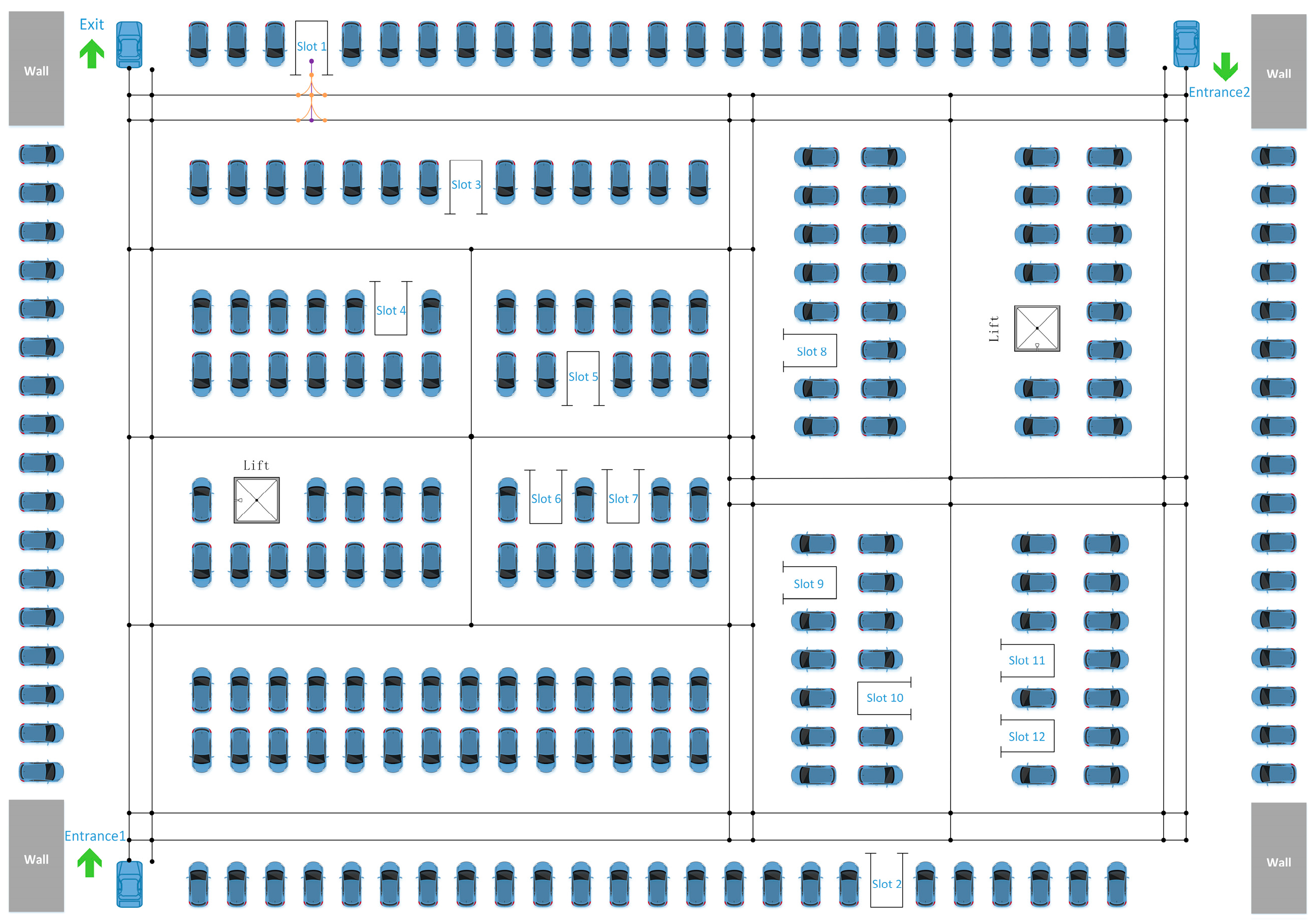
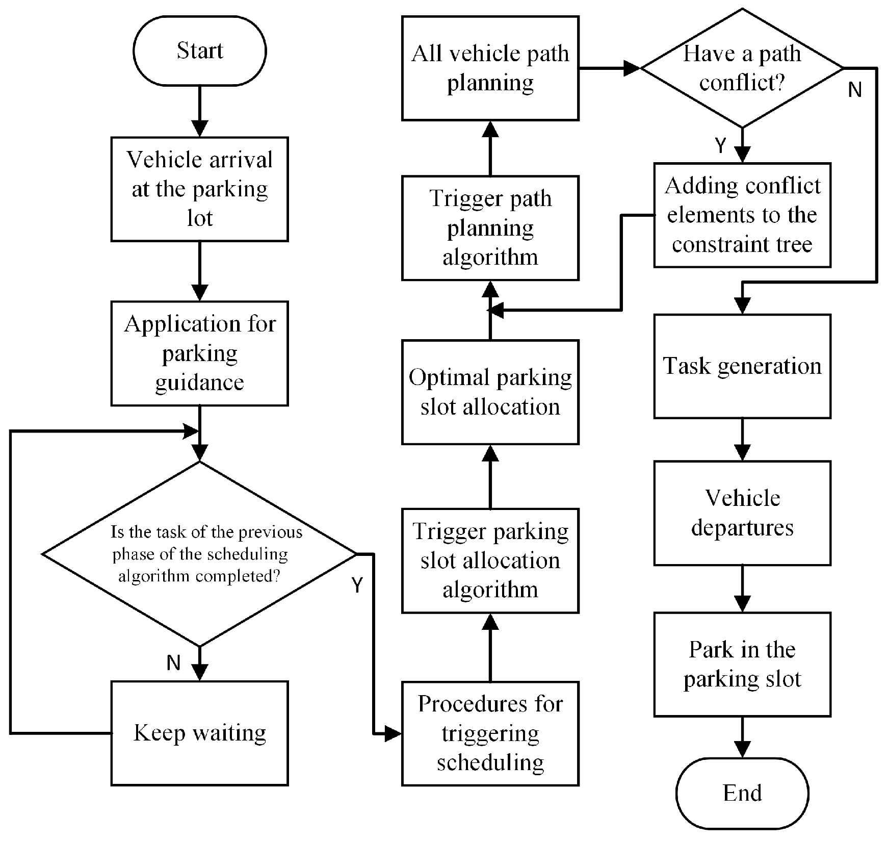
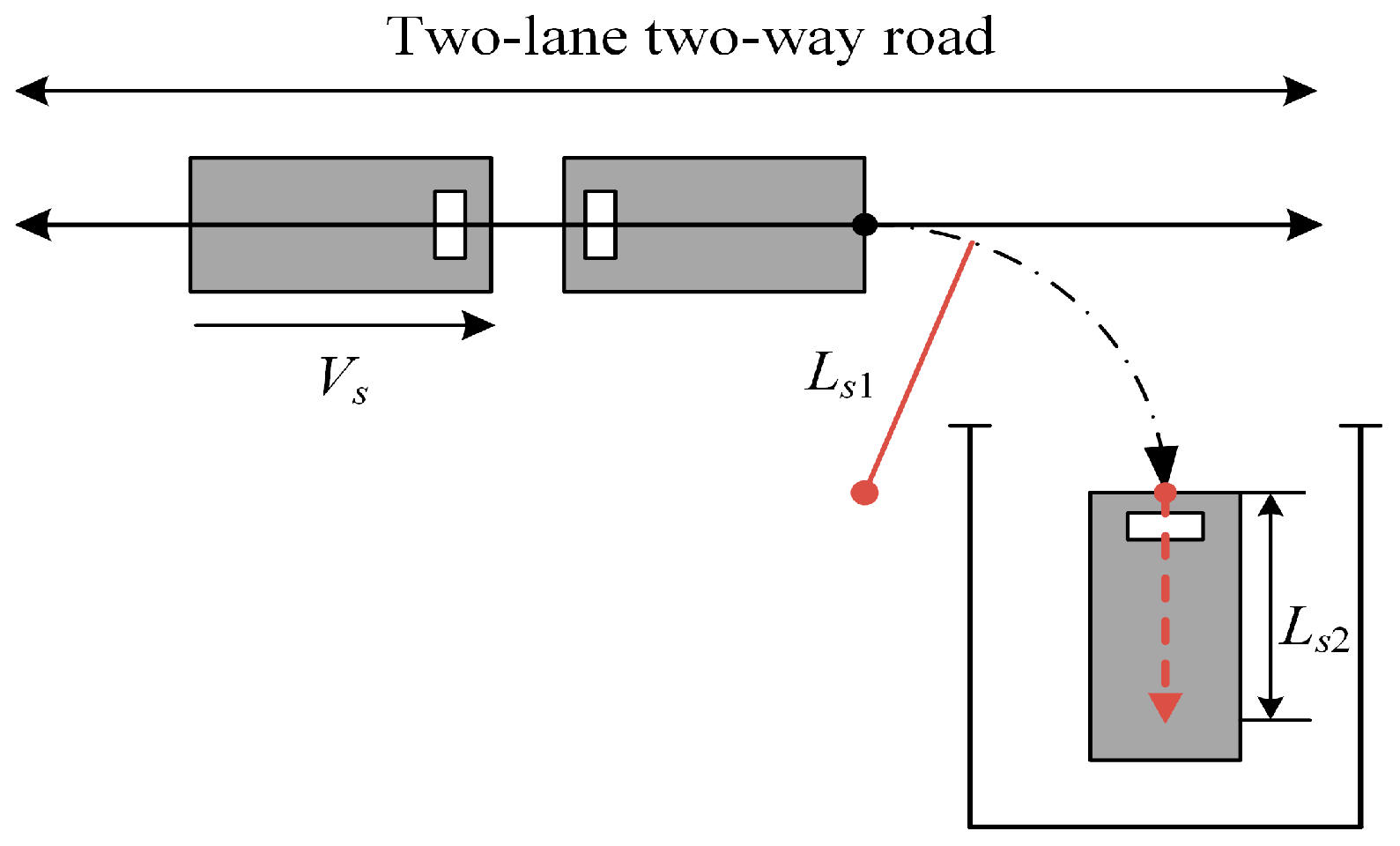
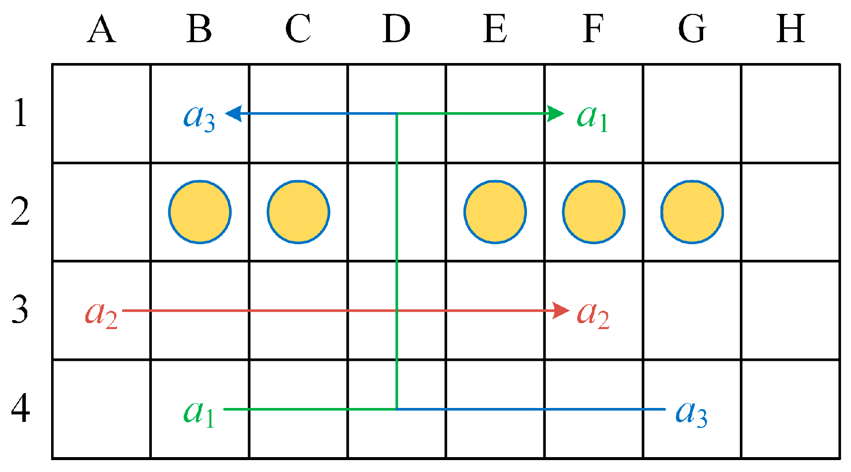
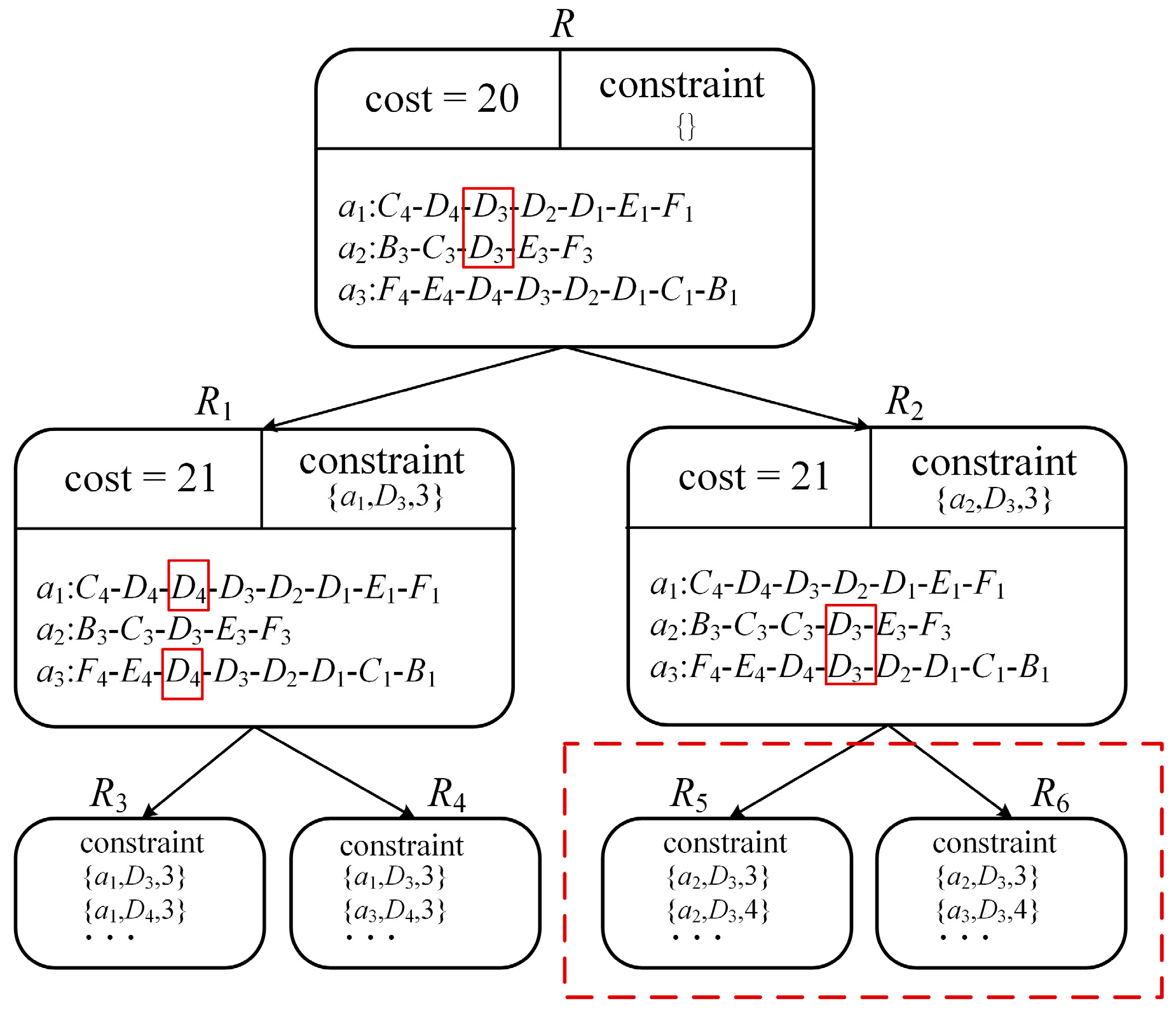
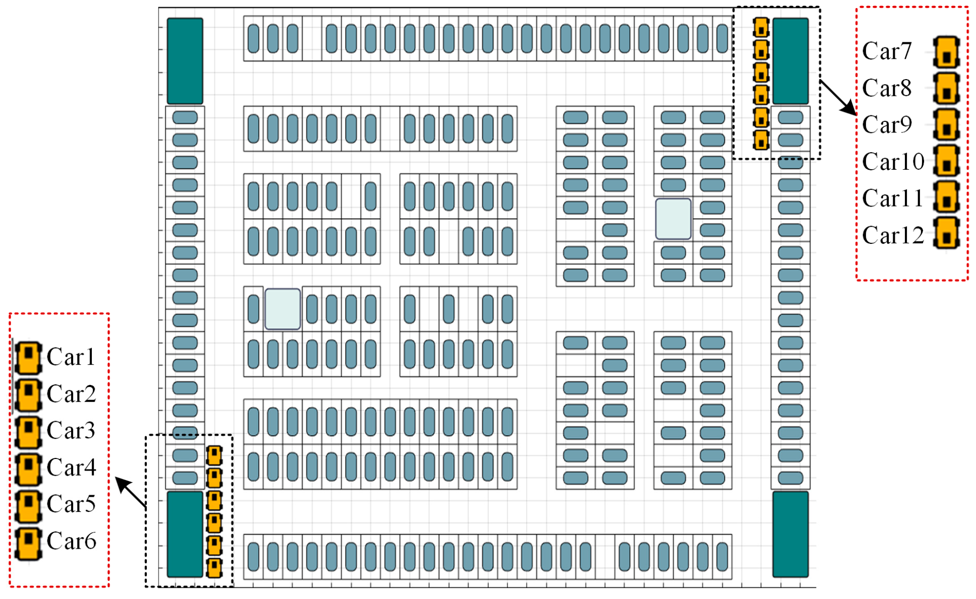
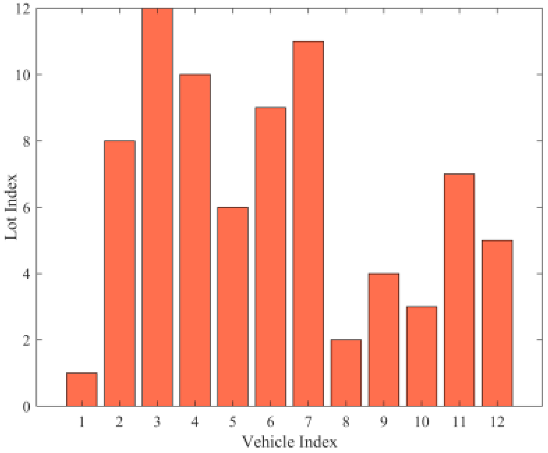
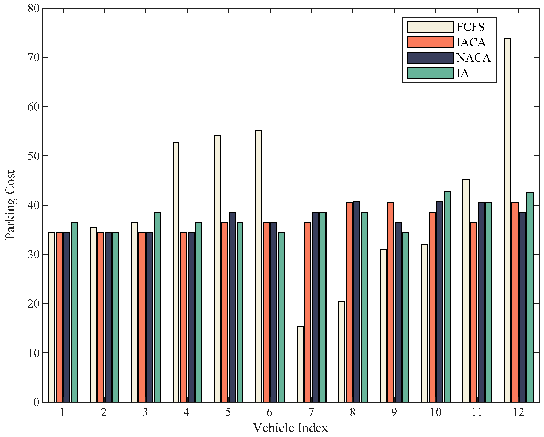
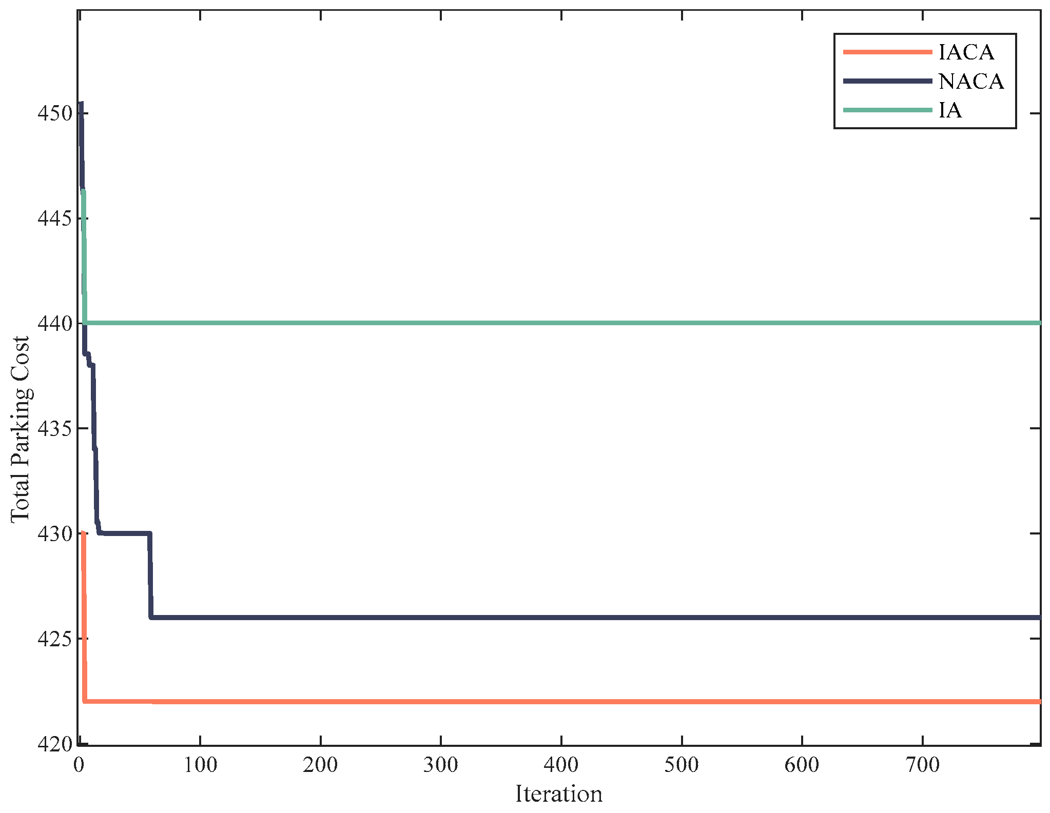
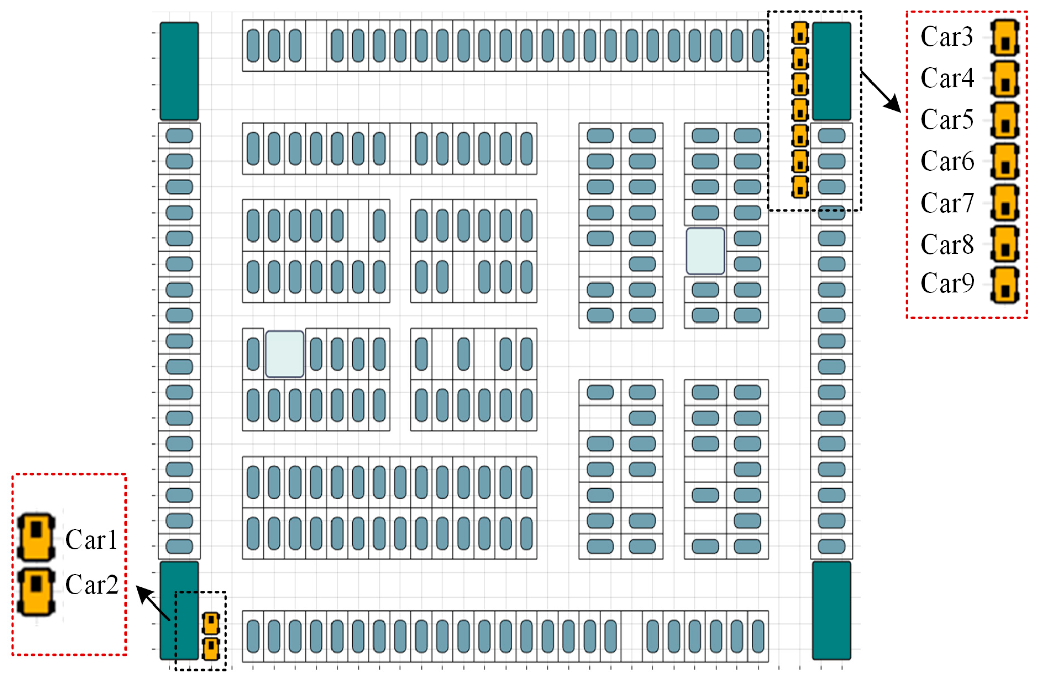

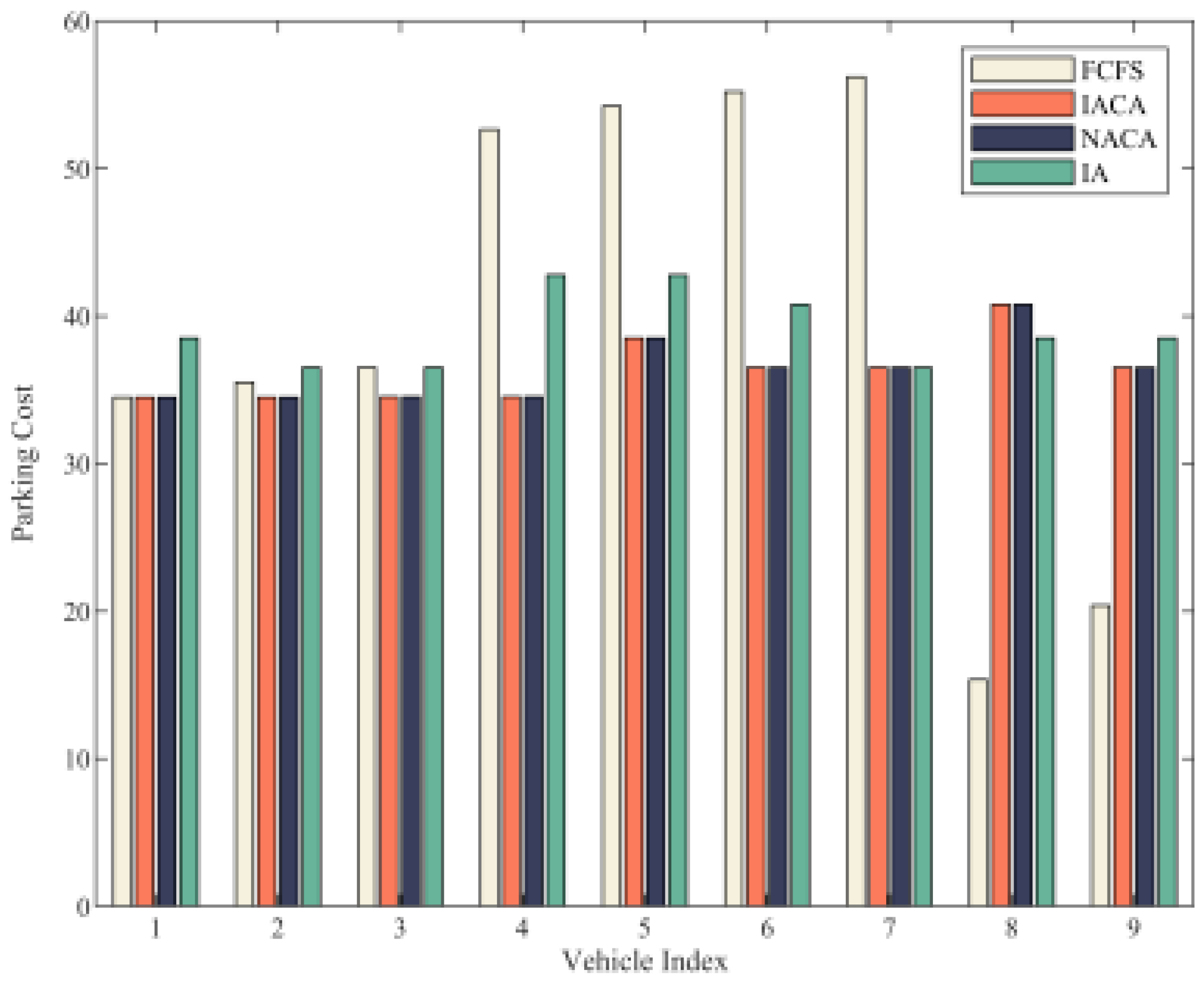

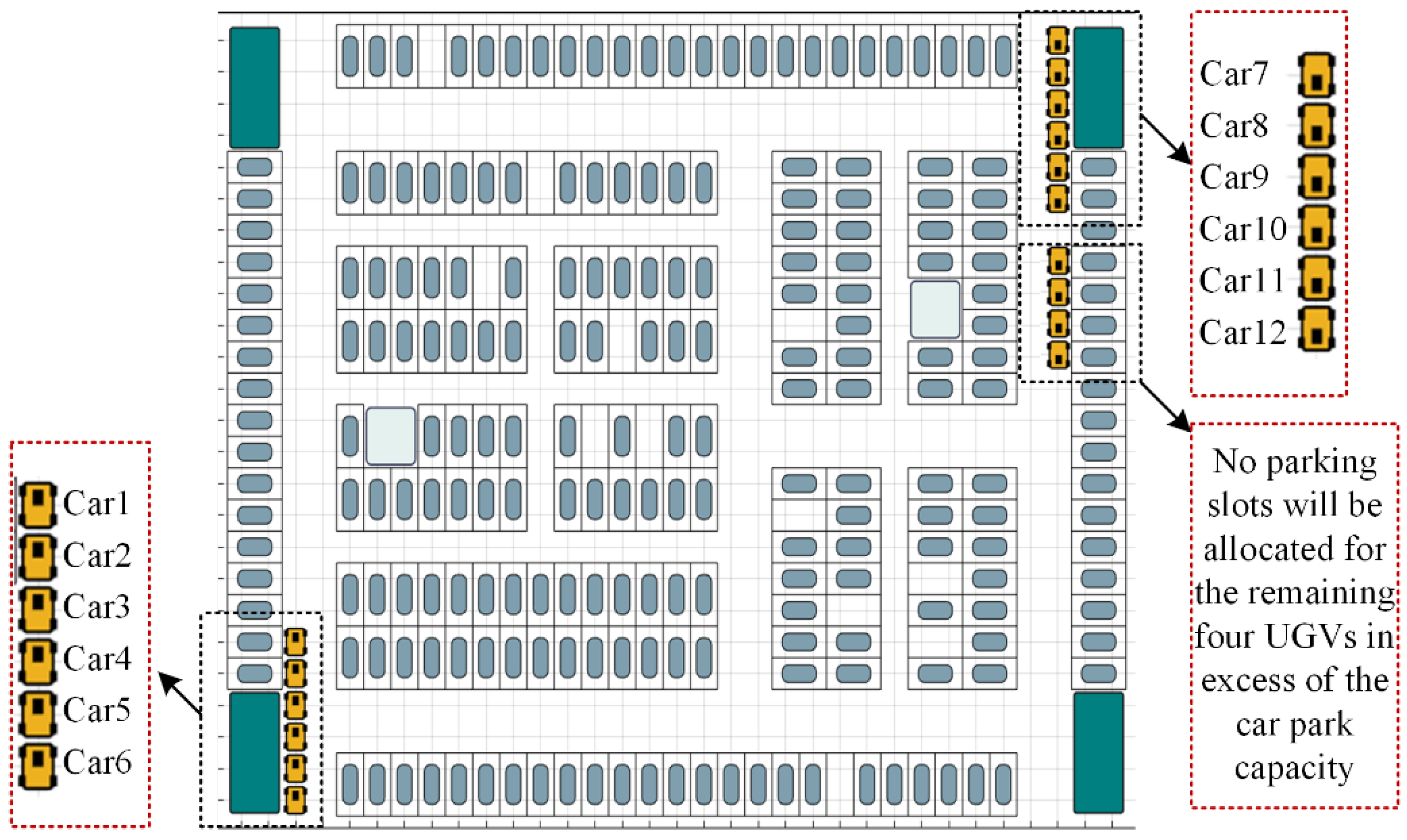
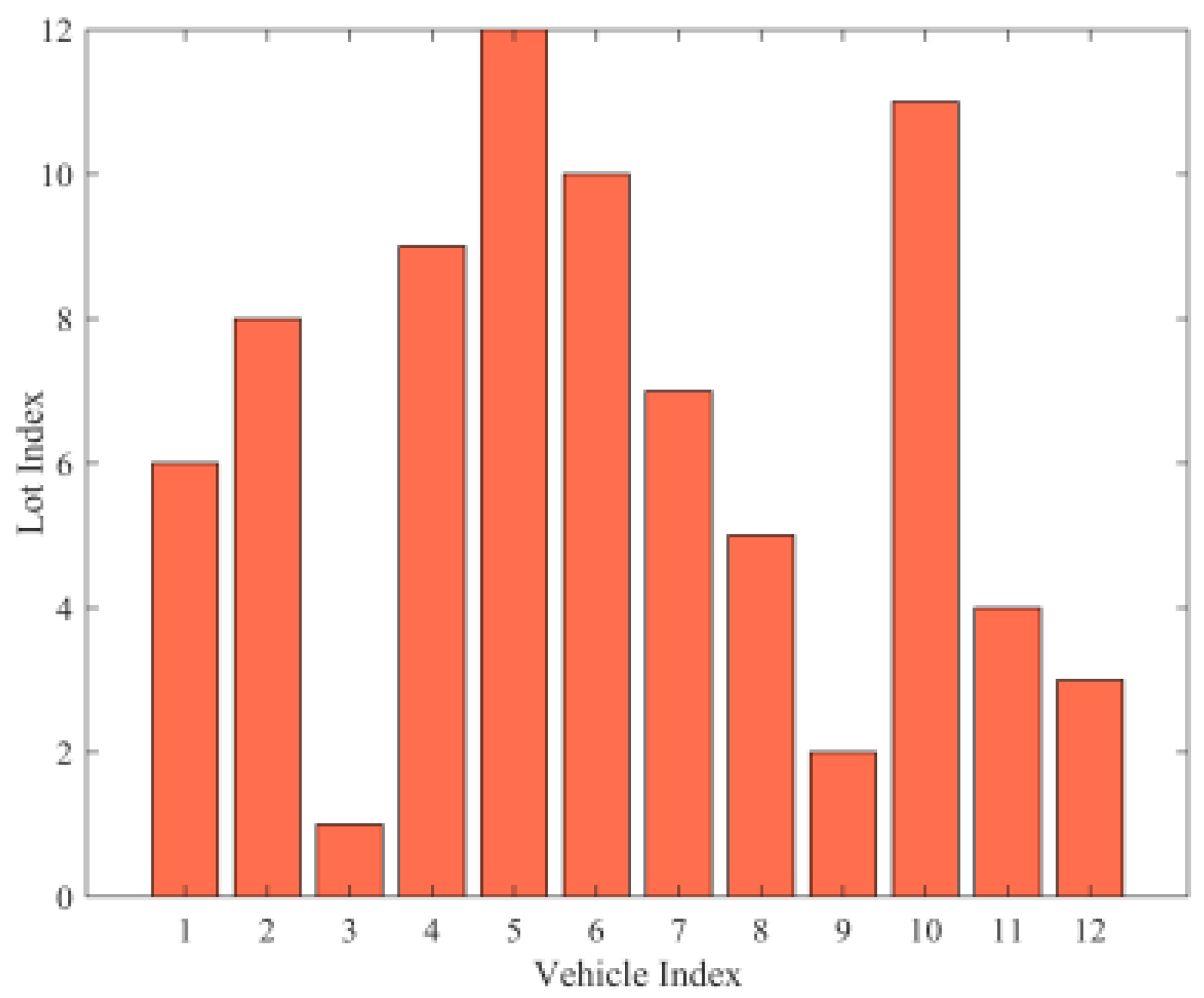
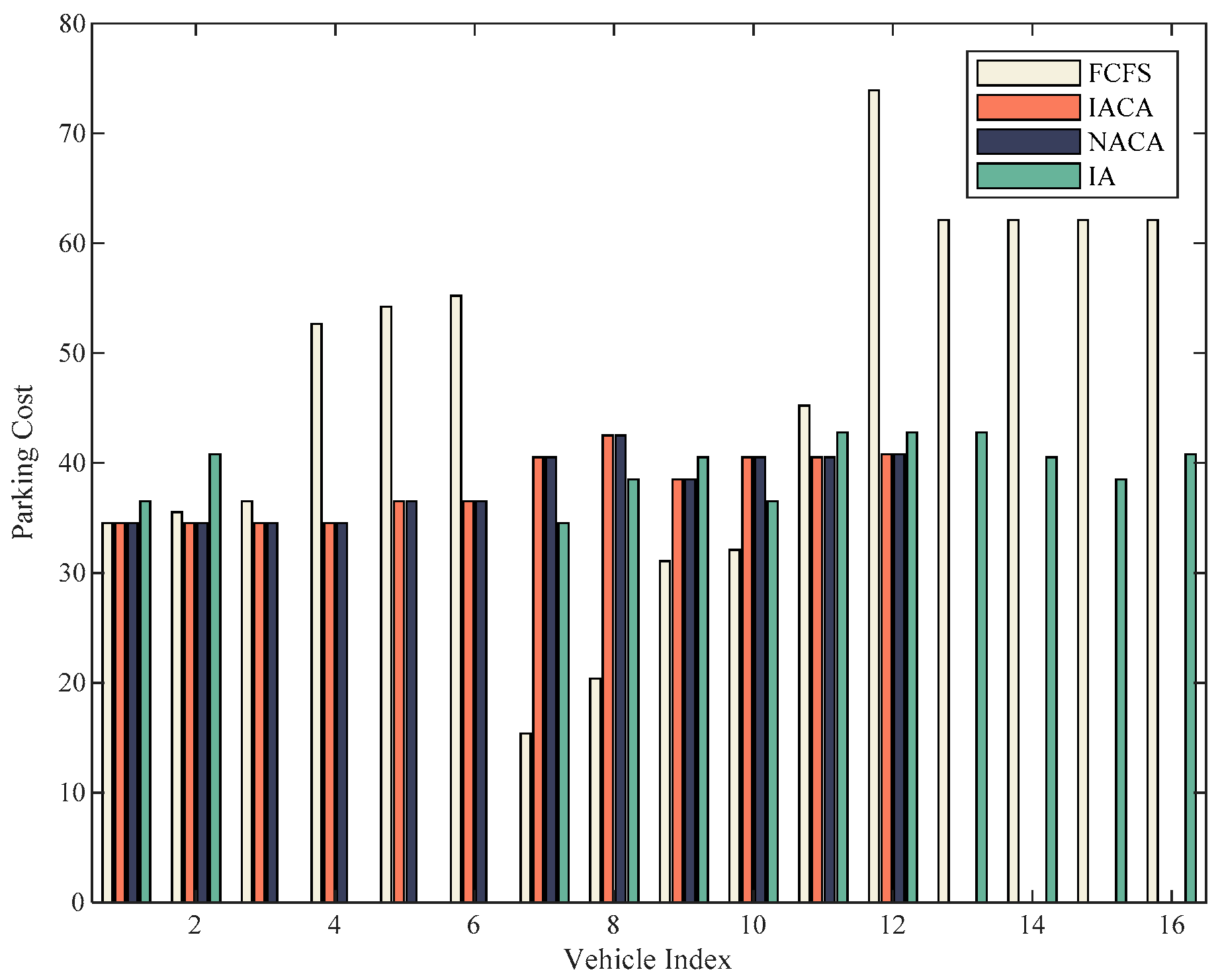
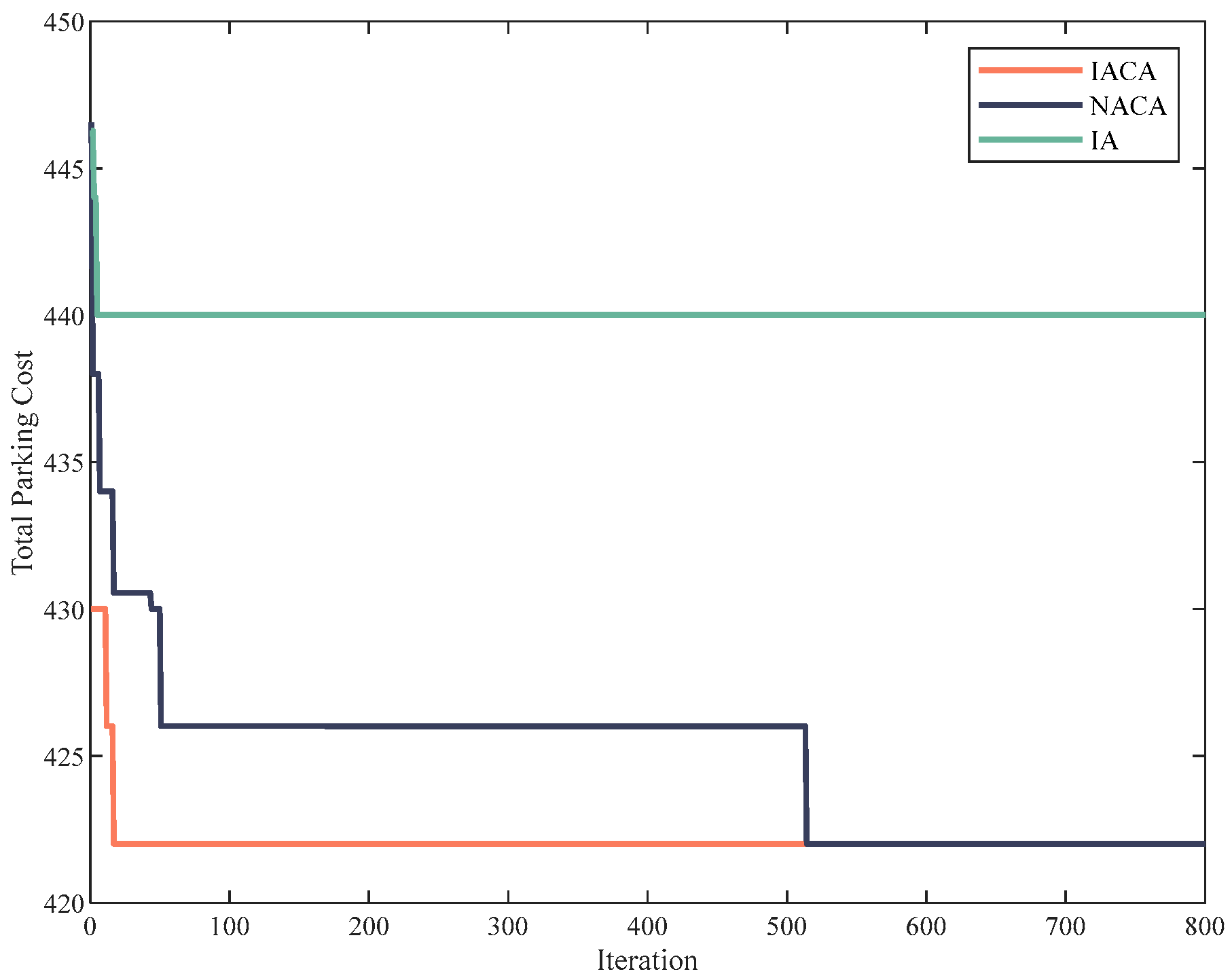
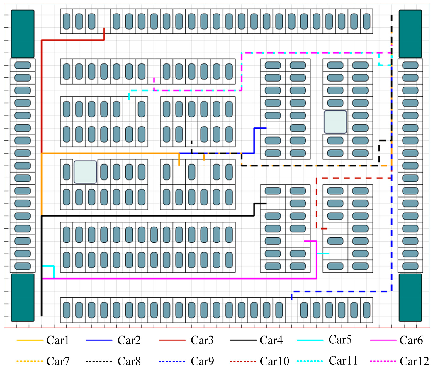


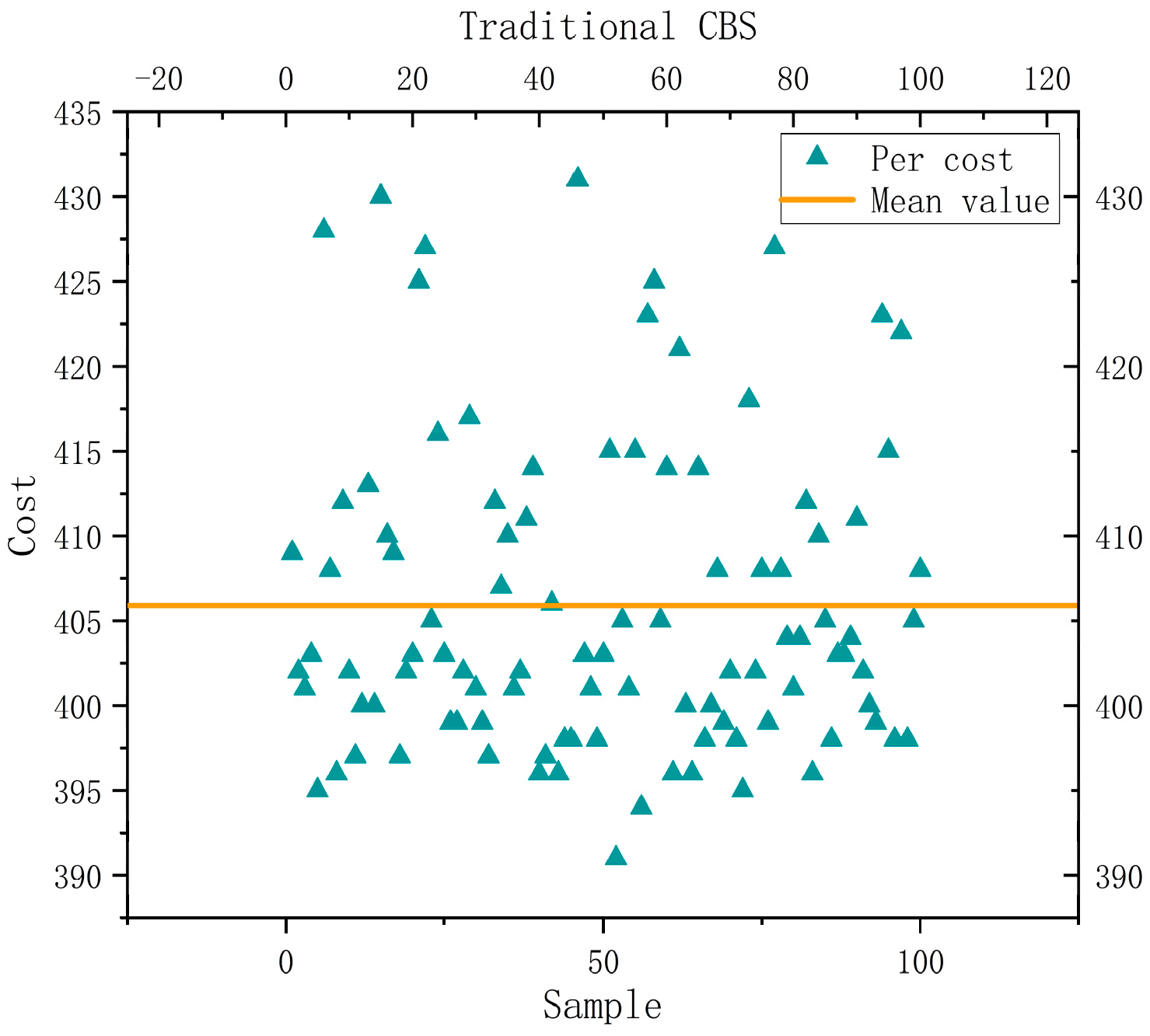
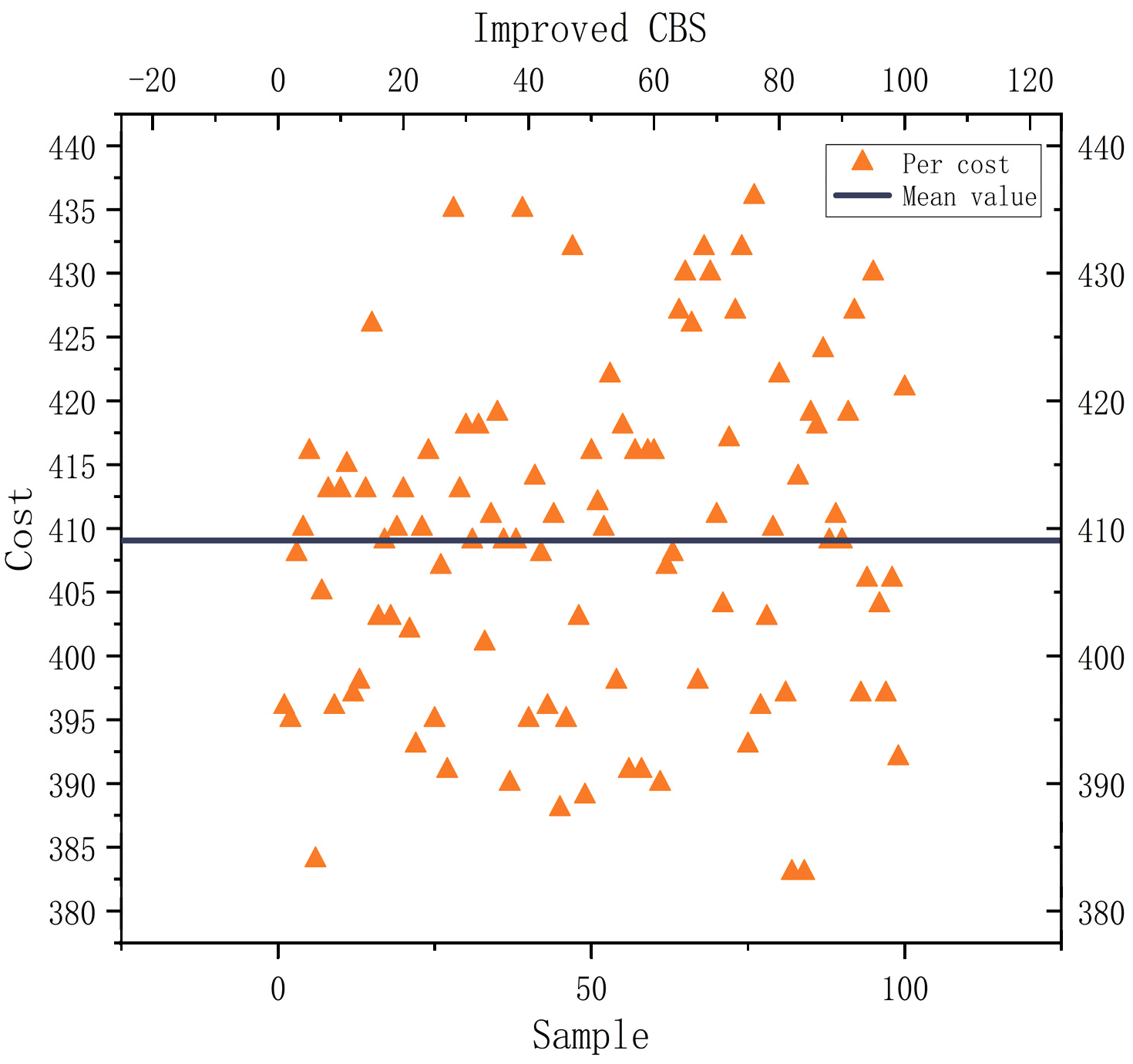
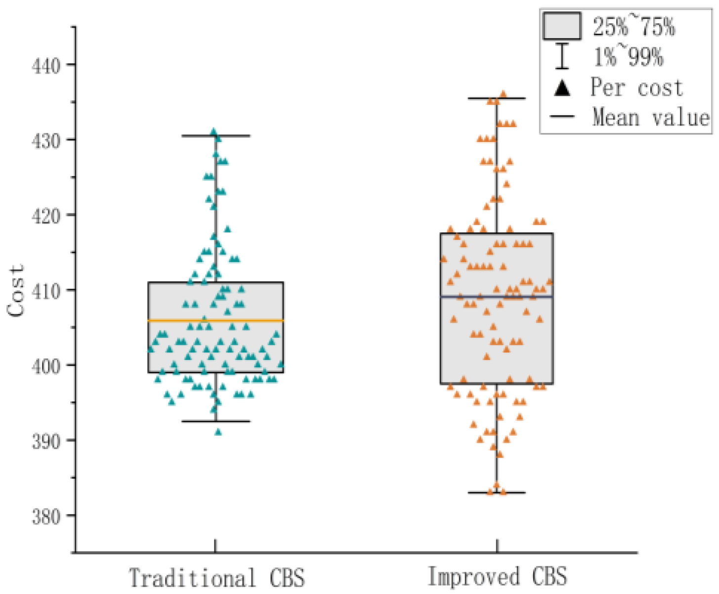
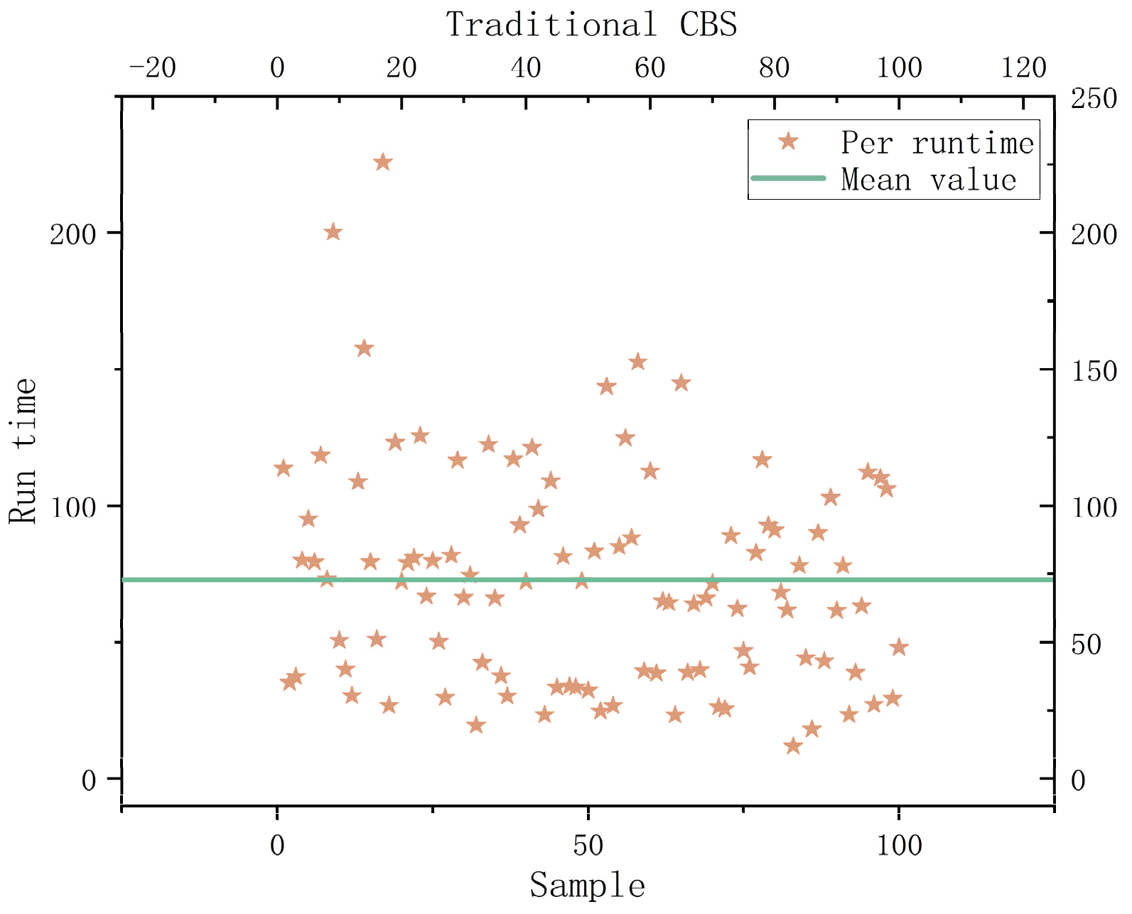
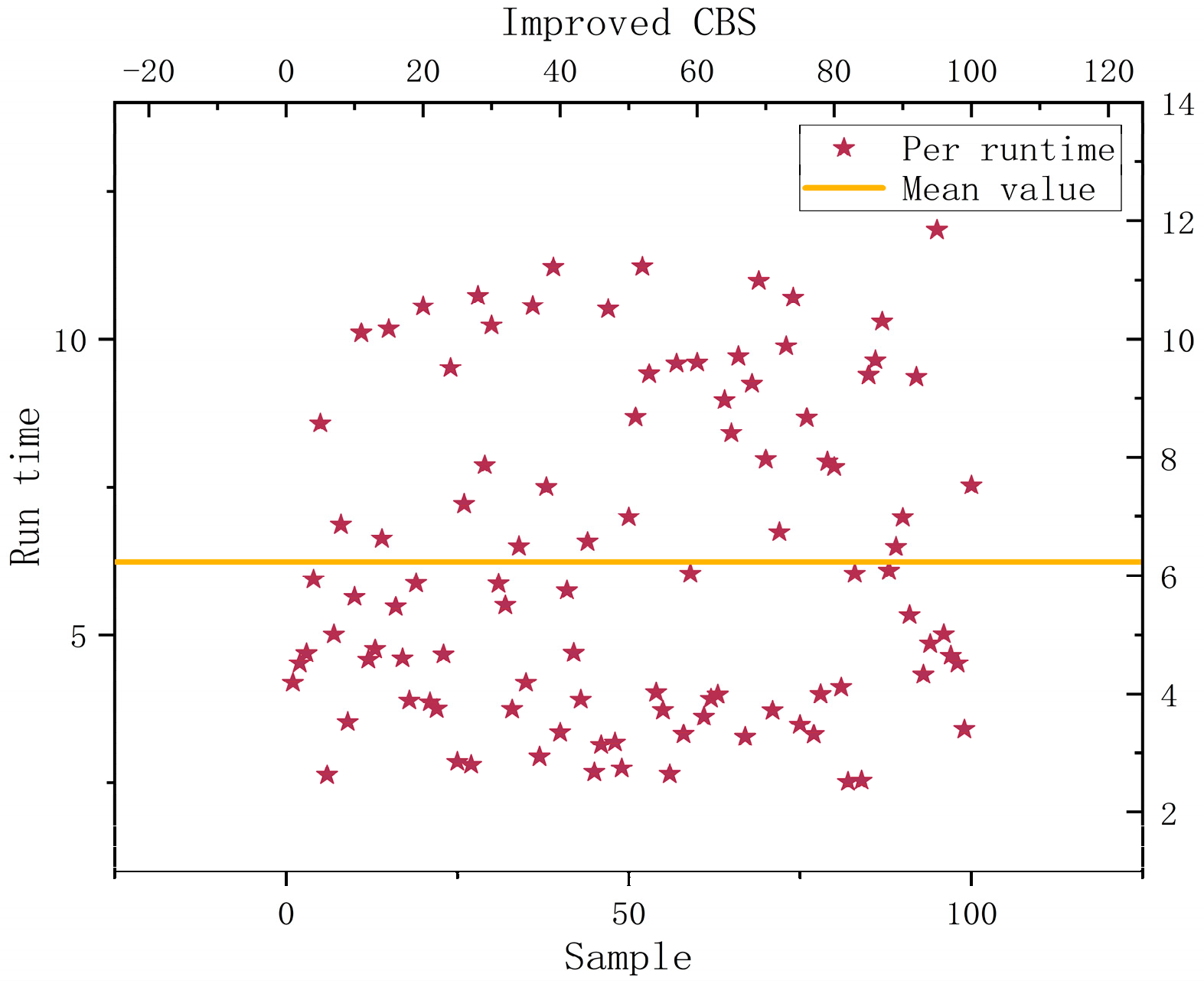
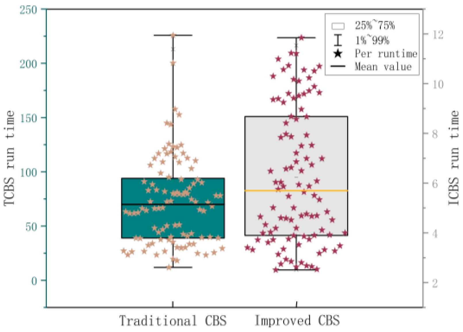
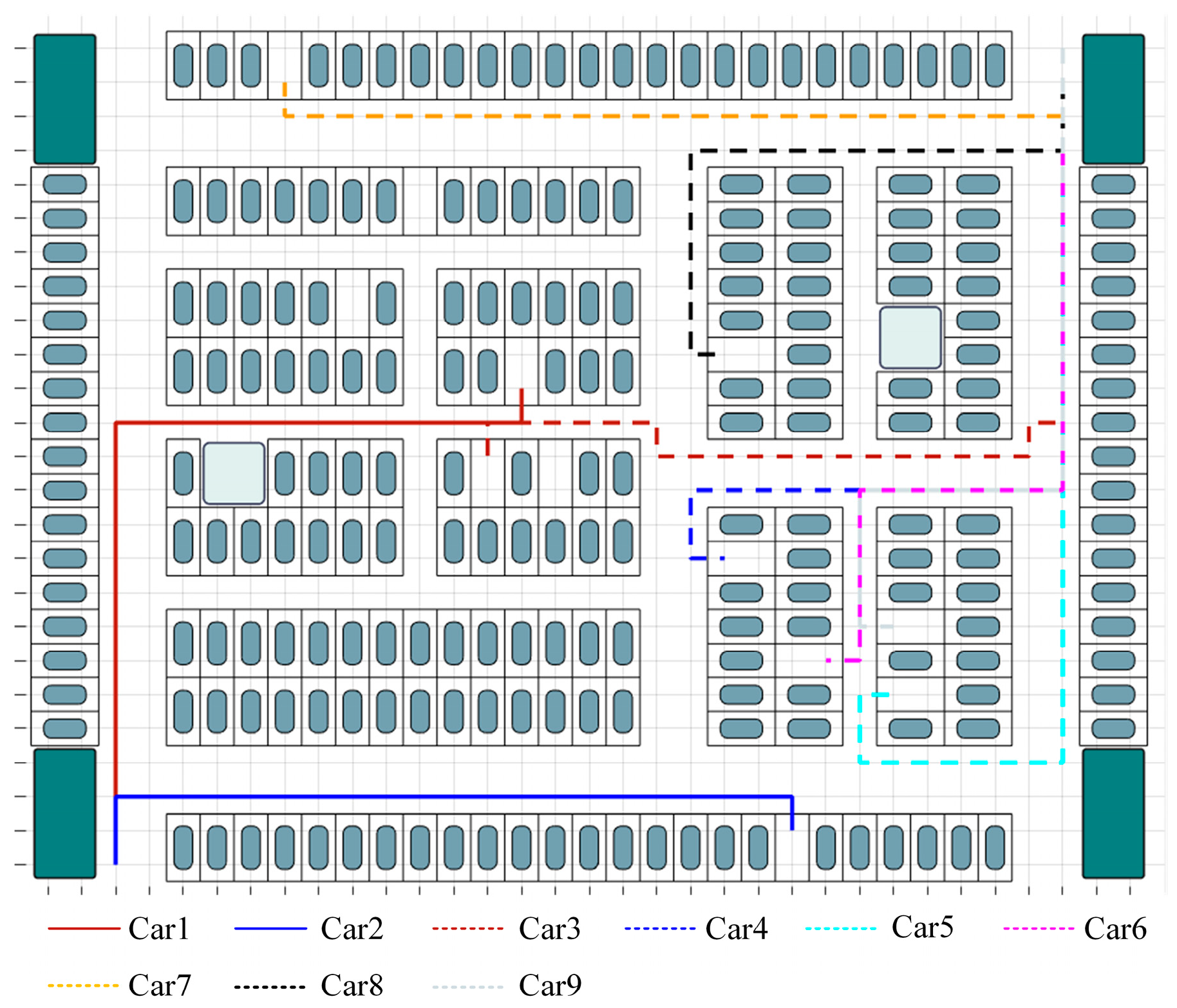
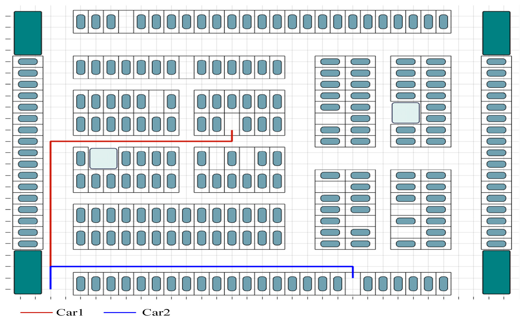
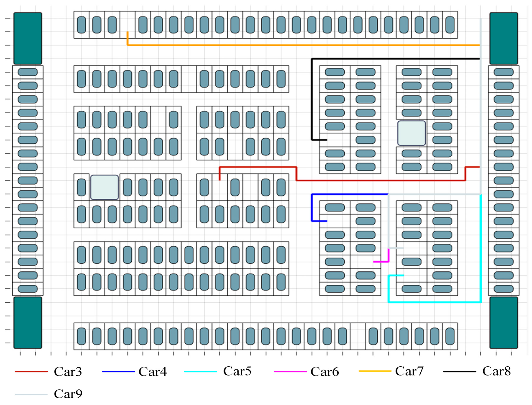

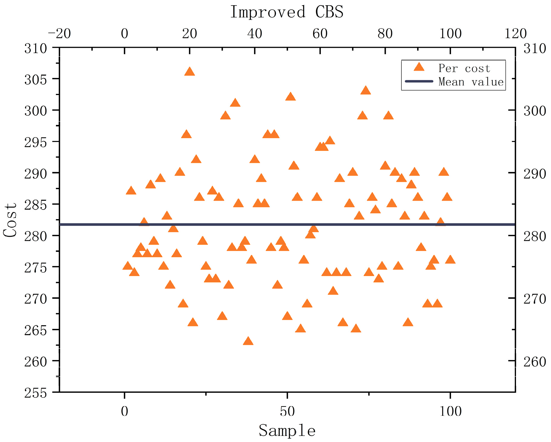
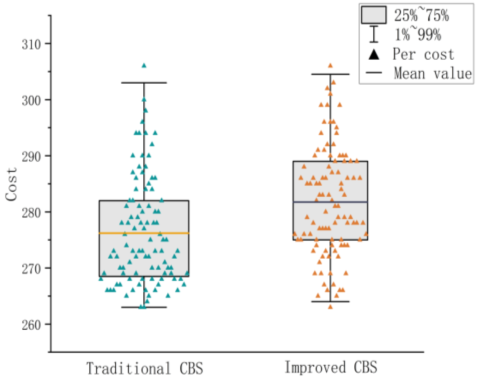
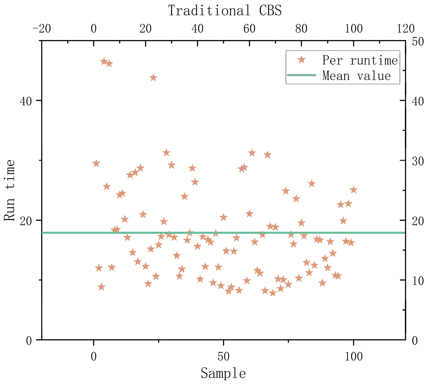
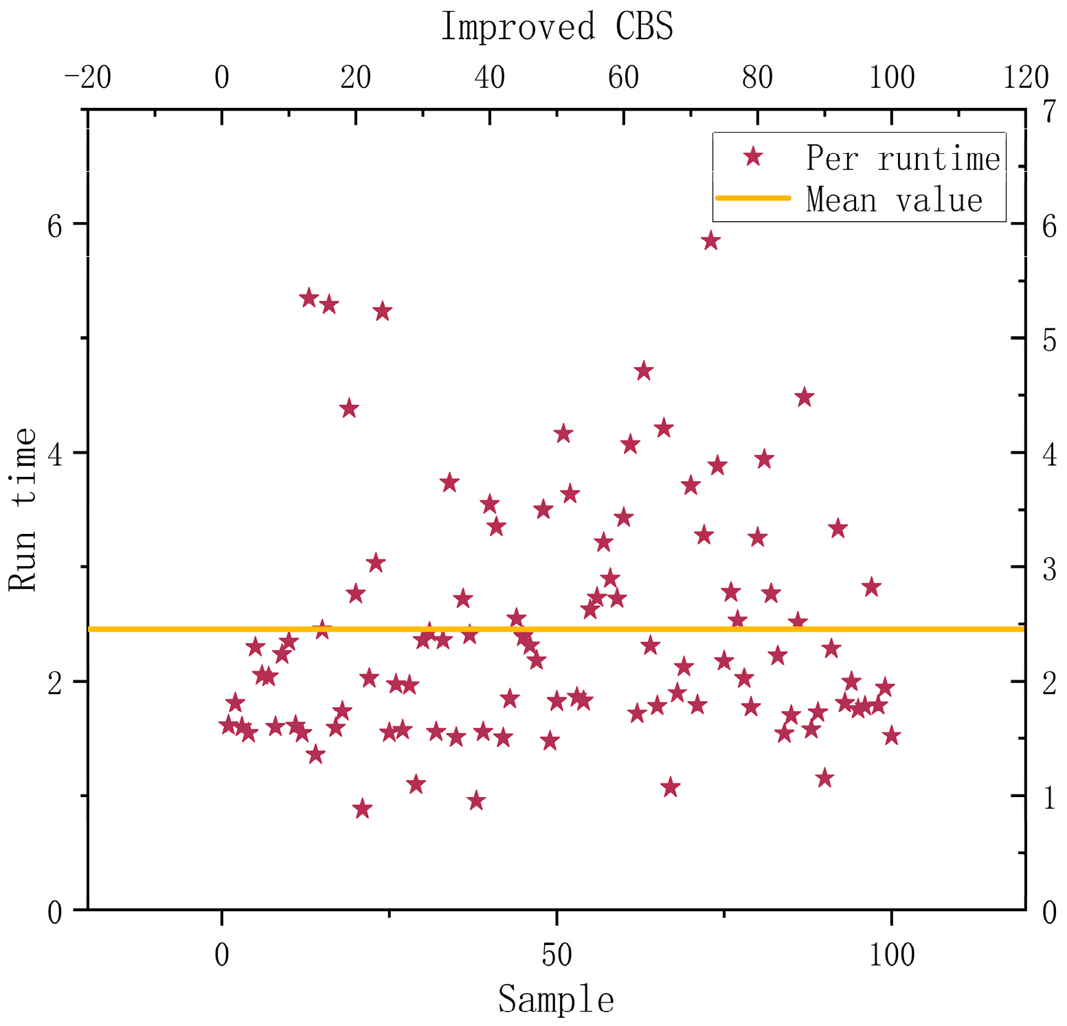


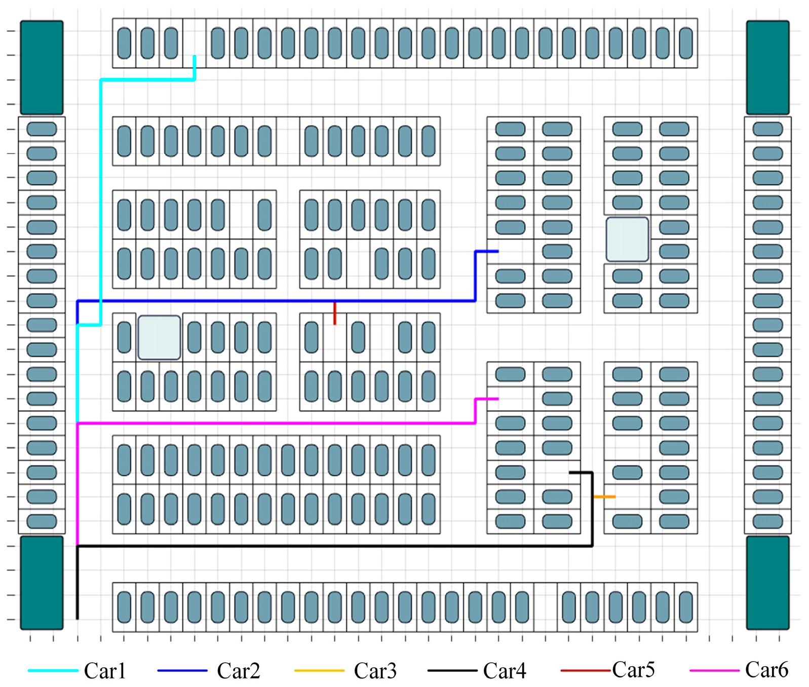
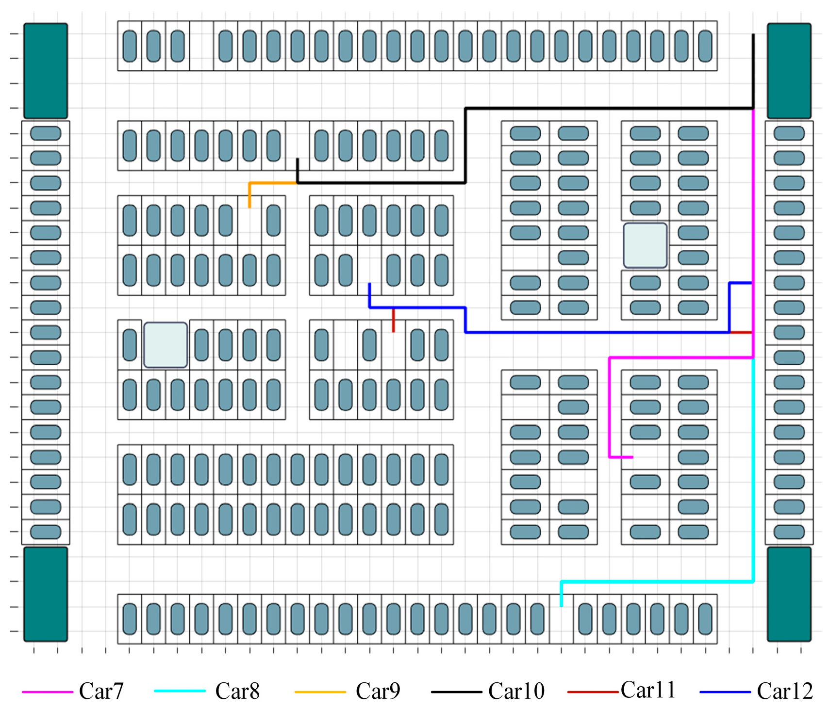
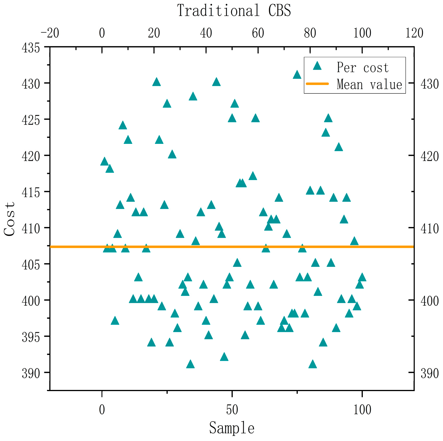
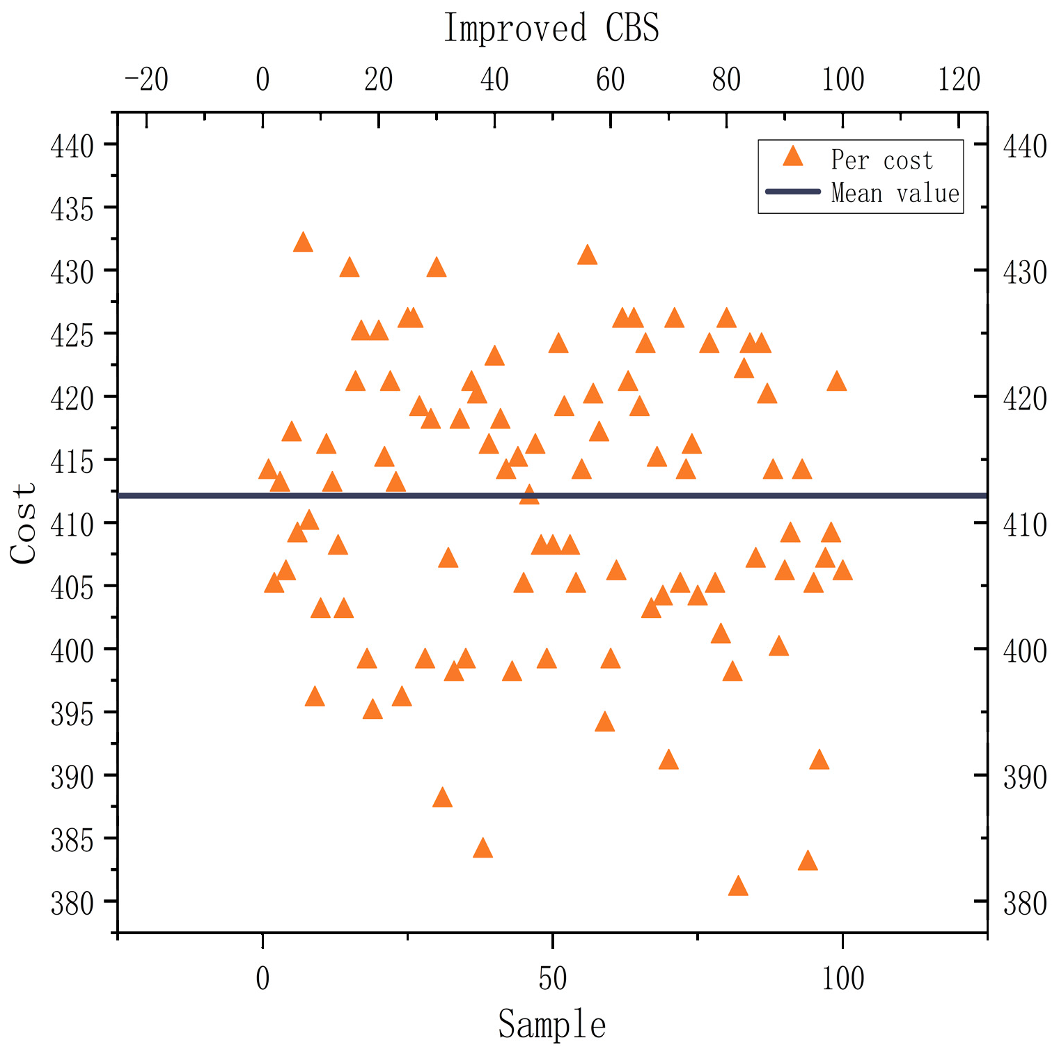
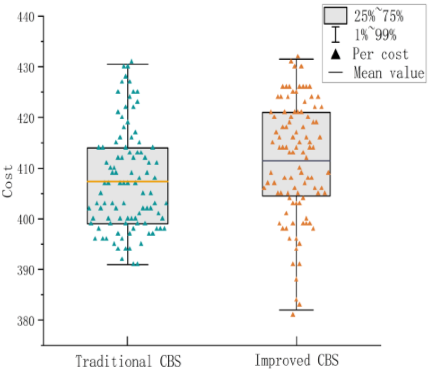
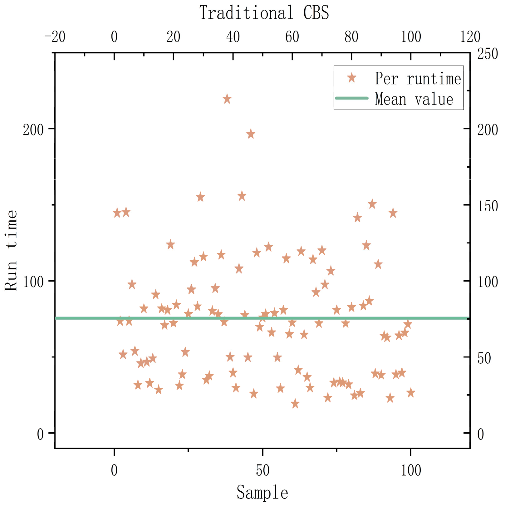
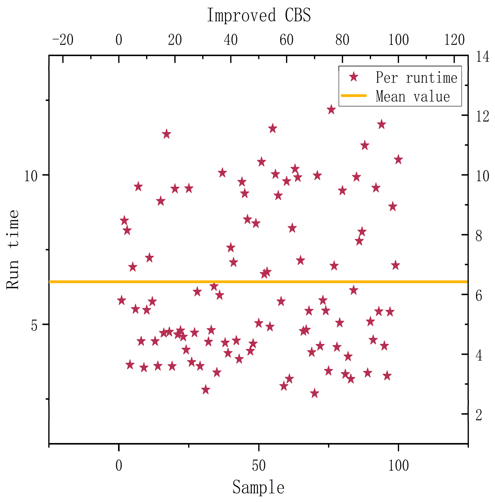
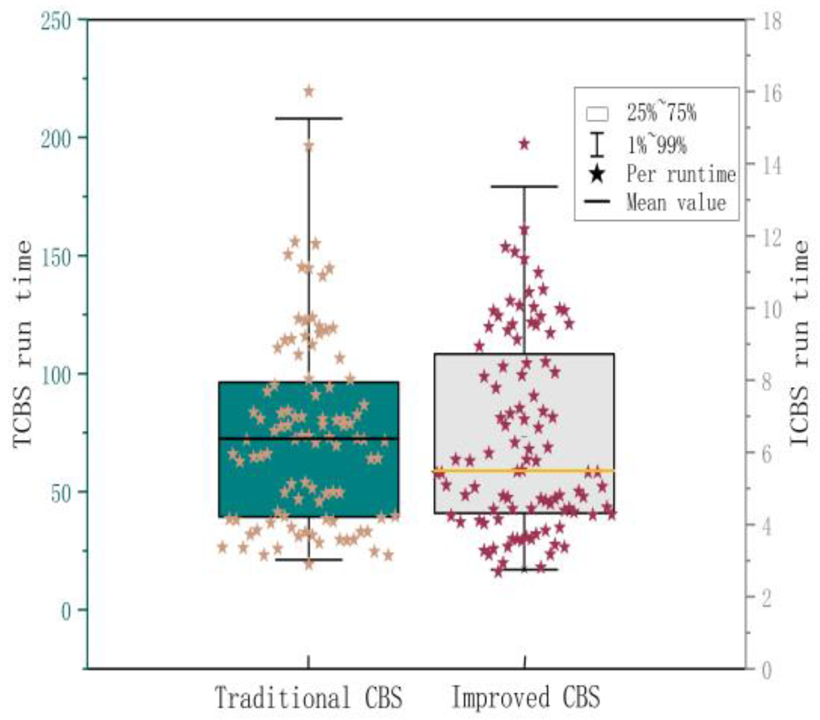
Disclaimer/Publisher’s Note: The statements, opinions and data contained in all publications are solely those of the individual author(s) and contributor(s) and not of MDPI and/or the editor(s). MDPI and/or the editor(s) disclaim responsibility for any injury to people or property resulting from any ideas, methods, instructions or products referred to in the content. |
© 2023 by the authors. Licensee MDPI, Basel, Switzerland. This article is an open access article distributed under the terms and conditions of the Creative Commons Attribution (CC BY) license (https://creativecommons.org/licenses/by/4.0/).