Author Contributions
Z.Z.: Conceptualization, Resources, Project administration, Funding acquisition. W.X.: Methodology, Software, Writing—original draft. G.X.: Resources, Software, Writing—original draft. S.X.: Methodology, Writing—original draft, Writing—review & editing. All authors have read and agreed to the published version of the manuscript.
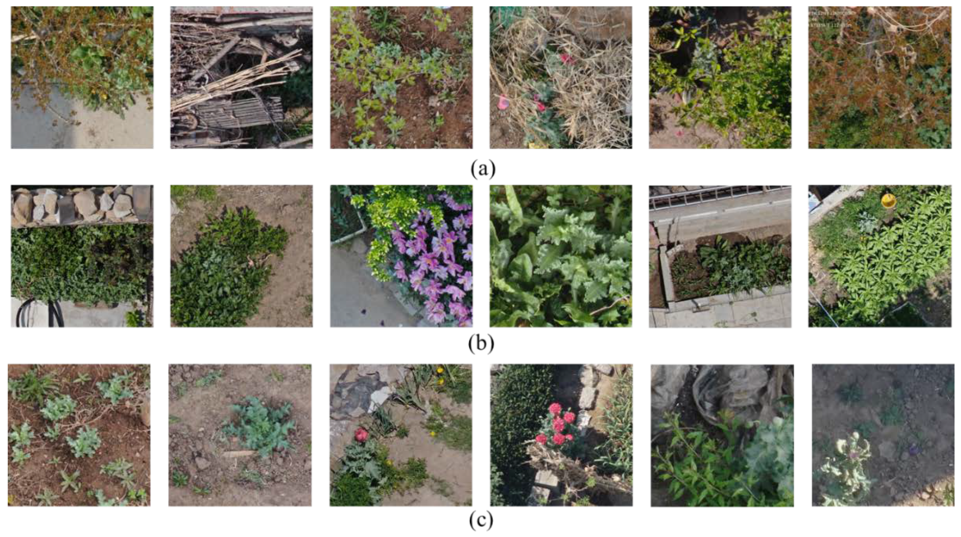
Figure 1.
Samples of opium poppies. (a) occlusion, (b) confused vegetation, (c) different growth periods.
Figure 1.
Samples of opium poppies. (a) occlusion, (b) confused vegetation, (c) different growth periods.
Figure 2.
Data collection and processing. The numbers 1–6 indicate the index of the block.
Figure 2.
Data collection and processing. The numbers 1–6 indicate the index of the block.
Figure 3.
Structure of the proposed HLA module.
Figure 3.
Structure of the proposed HLA module.
Figure 4.
Visualization comparison of feature maps for HLA input and output. The first row displays the input feature maps, while the second row showcases the visualized feature maps extracted by HLA.
Figure 4.
Visualization comparison of feature maps for HLA input and output. The first row displays the input feature maps, while the second row showcases the visualized feature maps extracted by HLA.
Figure 5.
The architecture of the proposed YOLOHLA. “↑” denotes the upsampling operation with the nearest interpolation, “↓” is the downsampling operation with convolution layer.
Figure 5.
The architecture of the proposed YOLOHLA. “↑” denotes the upsampling operation with the nearest interpolation, “↓” is the downsampling operation with convolution layer.
Figure 6.
Components of each module. “Conv” denotes the convolution layer, “BN” is the batch normalization, “SiLU” is the activation layer, “Concat” is the concatenation operation, and ⊕ is the addition operation.
Figure 6.
Components of each module. “Conv” denotes the convolution layer, “BN” is the batch normalization, “SiLU” is the activation layer, “Concat” is the concatenation operation, and ⊕ is the addition operation.
Figure 7.
Process of repetitive learning. The yellow circles represent missed detection objects, and the red circles represent false detection objects.
Figure 7.
Process of repetitive learning. The yellow circles represent missed detection objects, and the red circles represent false detection objects.
Figure 8.
Visual samples. The first, third, and fifth rows represent the feature response. The second, fourth, and sixth rows represent the detection results. The yellow circles represent missed detection objects.
Figure 8.
Visual samples. The first, third, and fifth rows represent the feature response. The second, fourth, and sixth rows represent the detection results. The yellow circles represent missed detection objects.
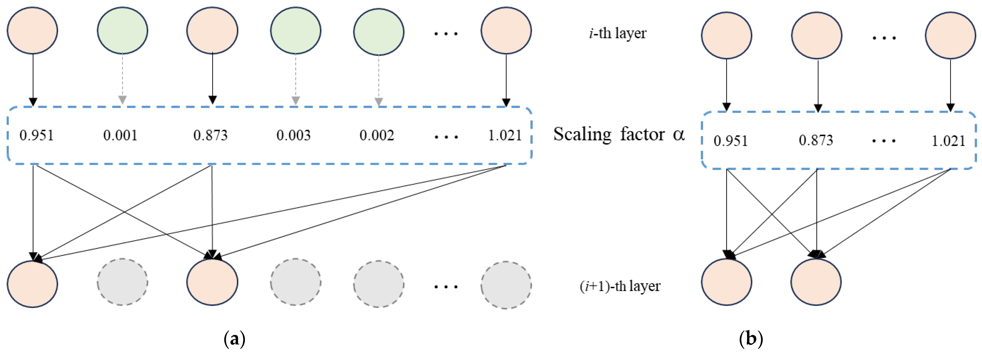
Figure 9.
Channel pruning process. The dashed lines represent channels with lower scaling factors, which will be discarded. (a) The sparsified model after sparse training. (b) The pruned model.
Figure 9.
Channel pruning process. The dashed lines represent channels with lower scaling factors, which will be discarded. (a) The sparsified model after sparse training. (b) The pruned model.
Figure 10.
Precision and Recall curves.
Figure 10.
Precision and Recall curves.
Figure 11.
Visualization results with different detectors. The dashed yellow circles represent the mis-detected objects, and the solid yellow circles represent the missed objects. (a) YOLOV5s. (b) YOLOV6-tiny. (c) YOLOV7-tiny. (d) YOLOHLA.
Figure 11.
Visualization results with different detectors. The dashed yellow circles represent the mis-detected objects, and the solid yellow circles represent the missed objects. (a) YOLOV5s. (b) YOLOV6-tiny. (c) YOLOV7-tiny. (d) YOLOHLA.
Figure 12.
Comparison of each convolutional layer before and after pruning. The X-axis shows the index of the convolution, and the Y-axis shows the number of channels of the convolution.
Figure 12.
Comparison of each convolutional layer before and after pruning. The X-axis shows the index of the convolution, and the Y-axis shows the number of channels of the convolution.
Figure 13.
Visualization comparison of object detection results after pruning. (a) Torch Pruning. (b) DepGraph. (c) Our method. The orange circles represent falsely detected objects. The yellow circle represents missed detection, and the orange circle represents false detection.
Figure 13.
Visualization comparison of object detection results after pruning. (a) Torch Pruning. (b) DepGraph. (c) Our method. The orange circles represent falsely detected objects. The yellow circle represents missed detection, and the orange circle represents false detection.
Figure 14.
Results from different baselines based on repetitive learning. Orange curve denotes the first method that divided dataset randomly. Blue curve denotes the second method that find the hard samples, but without prior knowledge. Green curve is the proposed RL method.
Figure 14.
Results from different baselines based on repetitive learning. Orange curve denotes the first method that divided dataset randomly. Blue curve denotes the second method that find the hard samples, but without prior knowledge. Green curve is the proposed RL method.
Figure 15.
Visual comparison (YOLOV5s is the baseline). (a) YOLOV5s. (b) YOLOV5s + HLA. (c) YOLOV5s + HLA + RL.
Figure 15.
Visual comparison (YOLOV5s is the baseline). (a) YOLOV5s. (b) YOLOV5s + HLA. (c) YOLOV5s + HLA + RL.
Table 1.
Comparison results with different detectors on the test dataset (Input size 640 × 640).
Table 1.
Comparison results with different detectors on the test dataset (Input size 640 × 640).
| Model | FLOPs | Param. | FPS | P | R | F1 | mAP |
|---|
| YOLOV4-tiny | 20.6 G | 8.69 M | 217 | 0.840 | 0.749 | 0.792 | 0.837 |
| YOLOV5s | 15.9 G | 6.70 M | 294 | 0.785 | 0.779 | 0.782 | 0.818 |
| YOLOV6-tiny | 36.5 G | 14.94 M | 169 | 0.882 | 0.861 | 0.871 | 0.873 |
| YOLOV7-tiny | 13.2 G | 5.74 M | 370 | 0.740 | 0.699 | 0.720 | 0.755 |
| YOLOV8s | 28.6 G | 10.65 M | 145 | 0.825 | 0.752 | 0.772 | 0.831 |
| PP-PicoDet | 8.3 G | 5.76 M | 251 | 0.808 | 0.734 | 0.769 | 0.792 |
| NanoDet | 3.4 G | 7.5 M | 196 | 0.784 | 0.744 | 0.763 | 0.714 |
| DETR | 100.9 G | 35.04 M | 117 | 0.812 | 0.763 | 0.787 | 0.852 |
| Faster R-CNN | 81.9 G | 36.13 M | 40 | 0.824 | 0.792 | 0.808 | 0.842 |
| RetinaNet | 91.0 G | 41.13 M | 41 | 0.813 | 0.828 | 0.820 | 0.795 |
| YOLOHLA | 13.8 G | 5.72 M | 323 | 0.839 | 0.770 | 0.803 | 0.842 |
| YOLOHLA + RL | 13.8 G | 5.72 M | 323 | 0.891 | 0.822 | 0.855 | 0.882 |
Table 2.
Comparative results with different pruning methods. (“Model size” refers to the number of bytes occupied by the model).
Table 2.
Comparative results with different pruning methods. (“Model size” refers to the number of bytes occupied by the model).
| Methods | P | R | F1 | mAP | FPS | Model Size |
|---|
| YOLOHLA | 0.839 | 0.770 | 0.803 | 0.842 | 323 | 20.8 MB |
| Torch pruning | 0.785 | 0.715 | 0.748 | 0.803 | 333 | 15.9 MB |
| DepGraph | 0.768 | 0.692 | 0.728 | 0.766 | 384 | 10.2 MB |
| YOLOHLA-Tiny | 0.843 | 0.731 | 0.783 | 0.834 | 456 | 7.8 MB |
Table 3.
Comparison results with different pruning methods on NVIDIA Jeston Orin platform (Input size: 640 × 640).
Table 3.
Comparison results with different pruning methods on NVIDIA Jeston Orin platform (Input size: 640 × 640).
| Methods | P | R | F1 | mAP | FPS |
|---|
| YOLOHLA | 0.839 | 0.770 | 0.803 | 0.842 | 128 |
| Torch pruning | 0.785 | 0.715 | 0.748 | 0.803 | 78 |
| DepGraph | 0.768 | 0.692 | 0.728 | 0.766 | 154 |
| YOLOHLA-Tiny | 0.843 | 0.731 | 0.783 | 0.834 | 172 |
Table 4.
Comparison results using YOLOV5s and different attention modules on the test dataset.
Table 4.
Comparison results using YOLOV5s and different attention modules on the test dataset.
| Model | P | R | F1 | mAP | FPS |
|---|
| YOLOV5s + SE | 0.795 | 0.730 | 0.761 | 0.795 | 278 |
| YOLOV5s + CA | 0.851 | 0.766 | 0.806 | 0.842 | 133 |
| YOLOV5s + ECA | 0.843 | 0.719 | 0.776 | 0.822 | 286 |
| YOLOV5s + CBAM | 0.840 | 0.720 | 0.775 | 0.819 | 294 |
| YOLOV5s + HLA | 0.839 | 0.770 | 0.803 | 0.842 | 323 |
Table 5.
Comparison results using YOLOV6-Tiny and different attention modules on the test dataset.
Table 5.
Comparison results using YOLOV6-Tiny and different attention modules on the test dataset.
| Model | P | R | F1 | mAP | FPS |
|---|
| YOLOV6-Tiny + SE | 0.901 | 0.829 | 0.864 | 0.870 | 169 |
| YOLOV6-Tiny + CA | 0.885 | 0.811 | 0.846 | 0.877 | 159 |
| YOLOV6-Tiny + ECA | 0.901 | 0.84 | 0.869 | 0.868 | 167 |
| YOLOV6-Tiny + CBAM | 0.906 | 0.829 | 0.866 | 0.866 | 159 |
| YOLOV6-Tiny + HLA | 0.908 | 0.851 | 0.878 | 0.882 | 154 |
Table 6.
Comparison of different pruning ratios. (“Model size” refers to the number of bytes occupied by the model).
Table 6.
Comparison of different pruning ratios. (“Model size” refers to the number of bytes occupied by the model).
| Pruning Ratios | P | R | F1 | mAP | FPS | Model Size |
|---|
| YOLOHLA | 0.839 | 0.770 | 0.803 | 0.842 | 323 | 20.8 MB |
| pr = 10% | 0.786 | 0.759 | 0.772 | 0.818 | 370 | 17.7 MB |
| pr = 20% | 0.782 | 0.568 | 0.658 | 0.72 | 385 | 14.5 MB |
| pr = 30% | 0.764 | 0.576 | 0.657 | 0.650 | 401 | 12.1 MB |
| pr = 40% | 0.670 | 0.502 | 0.574 | 0.544 | 417 | 9.8 MB |
| pr = 50% | 0.489 | 0.481 | 0.485 | 0.427 | 456 | 7.8 MB |
| Finetuning (pr = 50%) | 0.843 | 0.731 | 0.783 | 0.834 | 456 | 7.8 MB |
Table 7.
Comparisons of VisDrone2019 dataset.
Table 7.
Comparisons of VisDrone2019 dataset.
| Methods | P | R | F1 | mAP |
|---|
| YOLOV5S | 0.432 | 0.342 | 0.382 | 0.328 |
| YOLOV6-tiny | 0.476 | 0.4 | 0.435 | 0.371 |
| YOLOV7-tiny | 0.489 | 0.371 | 0.422 | 0.36 |
| YOLOHLA | 0.487 | 0.41 | 0.439 | 0.375 |


