Quadrotor Trajectory Control Based on Energy-Optimal Reference Generator

Abstract

Inspired by the limited battery life of multi-rotor unmanned aerial vehicles (UAVs), this research investigated hierarchical real-time control of UAVs with the generation of energy-optimal reference trajectories. The goal was to design a reference generator and controller based on optimal-control theory that would guarantee energy consumption close to optimal with lower computational cost. First, a least-squares-estimation-(LSE) algorithm identified the parameters of the UAV mathematical model. Then, by considering a precise electrical model for the brushless DC motors and rest-to-rest maneuvers, the extraction of clear rules to compute the optimal mission time and generate ’energetic trajectories’ was performed. These rules emerged from analyzing the optimal-control strategy results that minimized the consumption over many simulations. Afterward, a hierarchical controller tracked those desired energetic trajectories identified as sub-optimal. Numerical experiments compared the results regarding trajectory tracking, energy performance index, and battery state of charge (SOC). A co-simulation framework consisting of commercial software tools, Simcenter Amesim for the physical modeling of the UAV, and Matlab-Simulink executed numerical simulations of the implemented controller.

1. Introduction

1.1. Context

In recent years, UAVs have garnered widespread interest across diverse sectors, drawing attention from researchers, law enforcement, delivery firms, search-and-rescue teams, and agricultural enterprises. Their versatile applications have prompted extensive study and exploration within these varied industries. Furthermore, UAVs are evolving beyond their initial role in sensing activities, as highlighted in references such as [1,2], to play a crucial role in the execution of operational tasks. This shift underscores the expanding importance of UAVs, not only in data gathering but also in practical implementation operations. A growing area of research involves integrating manipulators with UAVs, enabling them to execute tasks like valve operations or collecting and placing objects. This interdisciplinary approach holds promise for enhancing the versatility of UAVs in various practical applications. Researchers emphasize that small UAVs, beyond manipulation capabilities, hold significant potential to advance research on remote sensing. The agility and accessibility of small UAVs could substantially enhance data collection and analysis in remote and challenging environments. In the coming years, a noticeable surge in experimental UAV applications is anticipated. Instances of this escalating interest include a Canadian company initiating drone-based payload deliveries [3], an Australian company launching coffee deliveries via drones [4], and successful tests of the use of drones for transport of organ transplants [5]. Additionally, UAVs are increasingly employed for transporting flexible linear objects, such as hoses and goods [6,7], and Swiss Post has utilized UAVs to transport medical samples, drastically reducing travel time from 45 min by car to just a few minutes of flight [7]. Furthermore, a recent study highlighted that UAV deliveries have the potential to contribute to a reduction in greenhouse-gas emissions associated with the freight industry [8]. This finding underscores the environmental benefits that innovative UAV applications could bring to the transportation sector.

The increasing demand for UAV applications underscores the need to enhance their efficiency, as highlighted in [9]. A substantial challenge in various applications is the constrained energy capacity of batteries or other power sources, even with the utilization of hybrid configurations. Currently, commercially available battery-powered multirotors offer an average flight time of 15 to 45 min, severely constraining their practical utility. This limitation underscores the pressing need for performance improvements in various aspects of UAV technology. In addition, the energy source must be shared among various applications, such as the high-consumption processes of video and image processing commonly installed on drones [10]. To address this challenge and to enhance overall efficiency, ongoing efforts are focusing on advancing energy sources, lightening drone components, optimizing energy utilization, and refining flight paths. Noteworthy measures include reducing UAV weight through the use of carbon-fiber structures and intelligent designs with high energy density, as well as improvements in the power-to-weight ratio. These initiatives are collectively contributing to making UAV systems more efficient and effective.

1.2. Relevant and Related Work

Indeed, power consumption in multirotors is a critical consideration, given their reliance on batteries with finite life spans. The heightened power usage primarily stems from the motors propelling the rotors to generate the thrust necessary for UAV flight [11]. The electrical energy consumed by these motors is contingent on the thrust demands and encompasses losses related to heat, friction, and the overall efficiency of the propulsion system. This efficiency factor encompasses losses in both the motors and the electronic speed controllers, contributing to the overall power-consumption dynamics of multirotor UAVs. Strategies to optimize power usage and enhance efficiency are crucial for extending flight times and improving the overall performance of these unmanned systems. In recent years, numerous research methods have been explored to address energy-saving challenges in UAVs. This includes investigations into the design of automatic battery recharging/replacement systems, aimed at enhancing the efficiency of power management. Additionally, efforts have been directed towards optimizing trajectories and control actions, seeking to minimize energy consumption during UAV operations. These multifaceted approaches reflect the ongoing commitment to developing innovative solutions that can contribute to energy savings, thereby extending the operational capabilities of unmanned aerial vehicles. The research in [12] introduced a battery-swapping mechanism designed to efficiently manage the resources and health systems of UAVs while reducing operator workload. This system not only facilitates the removal, charging, and installation of batteries but also incorporates an online algorithm capable of supervising the refueling of multiple UAVs simultaneously. The algorithm determines when a vehicle requires refueling and ensures a precision landing on the battery-swap mechanism’s landing pad. Another contribution in [13] presented the design, testing, and construction of an autonomous ground-based charging station specifically tailored for battery-powered quadrotor helicopters. Furthermore, studies in the same domain have explored enhanced methods of battery charging for multi-rotors, such as wireless charging [14,15]. In addition to recharging technologies, research efforts have focused on two key approaches to addressing energy constraints in transportation: optimizing the design stage of air transport and reducing energy consumption through efficient operational planning. These advancements collectively aim to improve the overall energy efficiency and autonomy of UAVs in various applications.

Energy savings in the design phase of UAVs can be achieved through various strategies, one of which involves minimizing the weight carried by the UAV. For small UAVs, where batteries can constitute up to 50% of the total mass [16], reducing additional payload mass becomes crucial for optimizing energy balance. Flying with an optimal mass can enhance UAV endurance and overall performance [17]. Additionally, hybrid designs, like the one proposed in [18], allow UAVs to travel on the ground when flight is unnecessary, contributing to energy conservation. The second approach to energy savings involves efficient movement planning, a focus of the research presented in this paper. This approach entails selecting a path with minimal energy consumption from multiple available paths generated by a route planner, as seen in [19]. The methodology in [19] employed offline energy-efficient route planning based on the Dijkstra algorithm, offering a systematic way to enhance the energy efficiency of UAVs during their operational phase. In the context of controlling paths with minimal energy consumption, the authors in [20] presented a stable path-following controller based on the simplified kinematic model of a quadrotor. Through various experiments, they demonstrated the effective performance of this controller under both constant and variable desired speed profiles. The variable speed profile in this case was defined by the geometric requirements of the predetermined path. Moreover, significant research has delved into the application of real-time-dynamic-programming-(RTDP) techniques for drones, as highlighted in [21]. The optimization algorithm developed in this work drew inspiration from a dynamic real-time programming approach introduced in [22], originally designed for speed optimization to minimize energy consumption in automobiles. These advancements have contributed to the ongoing efforts to develop efficient and adaptive control strategies for UAVs, particularly in the context of energy-aware path planning.

The work in [23] introduced a quadratic programming approach for trajectory generation in aerial manipulators. Although effective, a significant drawback was evident, in terms of the computational burden and energy consumption, particularly when implemented on board. Similarly, in [24], the determination of the best trajectory for a quadrotor aerial vehicle between two hover configurations was explored in the context of energy consumption. The study examined three types of smooth trajectories: minimum snap, minimum jerk, and minimum acceleration. However, the minimization problem in this work did not account for a specific model, and estimation of optimal mission time was not provided, differing from the approach presented in the current work.

In a recent publication [25], a method was introduced for designing a dynamic model that enables the estimation of energy consumption in quadrotors. This model was specifically developed to analyze the energy efficiency of the quadrotor during different maneuvers. In the domain of fixed-wing UAVs, [26] explored an energy-efficient control method based on determining flight trajectories using a hexagonal grid. This investigation contributed to the ongoing efforts to enhance the energy efficiency and autonomy of unmanned aircraft systems through advanced control strategies. In [27], minimum energy paths were established for a quadrotor between initial and final states by solving an optimal control problem using the UAV model. Additionally, a trajectory of minimum time and/or minimum control effort was computed through the solution of a relative optimal-control problem. However, the approach outlined in this study was executed offline, and its lack of feedback made it impractical for certain applications. One potential solution is periodic utilization, computing optimal trajectory references with feedback. However, this approach, while less intensive than dynamic programming, still incurs notable energy consumption and requires instruments with excellent processing capabilities.

In recent years, numerous studies have focused on reference generation, recognizing its impact on energy consumption. In [28], the researchers investigated a trajectory-planning algorithm for a UAV, considering constraints on the accuracy of the system positioning. Another study by [29] formulated trajectory generation as a quadratic-programming problem with linear constraints, specifically addressing the challenge of performing aggressive maneuvers with quadrotors. Additionally, ref. [30] presented a path-planning generation algorithm that incorporated the evolution of battery performance. This approach involves computing the battery state of health (SoH) through degradation models and formulating the path-planning algorithm as a multi-objective optimization problem. The objective is to find a feasible trajectory between waypoints while minimizing energy consumption and mission time, accounting for variations in the battery SoH. These investigations have collectively contributed to the ongoing efforts to enhance energy-efficient reference generation for UAVs. In [31], in order to improve the efficiency of UAVs in transmission-tower inspections, a UAV transmission-tower-inspection energy-consumption model was proposed for the existing research, in which there was no accurate energy-consumption-calculation method in transmission-tower inspection, and the optimal energy consumption path for UAV transmission tower inspection was designed in combination with the simulated annealing algorithm. An approach to modeling the full translational dynamics of a quadrotor UAV by a feedforward neural network was proposed by [32], which was adopted as the prediction model in a model predictive controller (MPC) for precise position control. Finally, the aim of [33] was to shed light on the problem of shaping control signals in terms of energy-optimal flights. The synthesis of a UAV autonomous control system with a brain-emotional-learning-based intelligent controller (BELBIC) is presented.

1.3. Original Contributions and Organization

It is a valid point that, in many published works, the dual perspective of both energy efficiency and computational feasibility has not been thoroughly addressed. While setting the problem as an optimal control problem with diverse objectives is crucial for energy optimization, practical considerations related to computational efficiency and cost sustainability at the application level are often overlooked. Our research approach, focusing on both energy and computational aspects, provides a unique and comprehensive viewpoint that is essential for addressing real-world applications. This dual perspective is likely to contribute significantly to a more holistic understanding and solution to the challenges faced in optimizing UAV operations.

Our research contribution, as described, is valuable in providing optimal mission time and trajectory generation rules for drones that are not only energy-efficient but also computationally feasible. The emphasis on simplicity in calculations and proximity to optimal solutions is particularly noteworthy, as it facilitates the implementation of real-time hierarchical control with low computational demands. This approach addresses the practical challenges associated with deploying UAVs in real-world scenarios, where both energy efficiency and computational efficiency are crucial factors. This work has the potential to significantly impact the field by offering a practical and effective solution for optimizing UAV operations, in terms of both energy consumption and computational resources. The methodology adopted in our research is notable, starting with the identification of unknown quadrotor parameters through the least-squares method applied to experimental data. Subsequently, the derivation of mission time and trajectory generation rules, close to optimal in terms of energy consumption, represents a unique and practical approach. The inspiration drawn from [34], though initially related to the automotive domain, demonstrates innovative thinking in adapting such methodologies for UAVs. The emphasis on estimating the optimal mission time without directly solving the optimal control problem is a noteworthy contribution. This aspect, which is crucial for energy efficiency, has not been extensively explored in the existing literature. Our work addresses this gap by providing a novel perspective on the significance of mission time in energy consumption, offering valuable insights for optimizing UAV operations. The identification of simple rules for reference generation, once the mission time is selected, adds a practical dimension to the research, making it applicable in real-time scenarios with reduced computational demands. The dual emphasis on energy efficiency and computational feasibility enhances the practical applicability of our work in the realm of UAV operations. The final phase of our research, which involved comparing controller performance on trajectory control using a commercial simulator, added a practical validation aspect to our work. Evaluating energy consumption in terms of battery state of charge (SOC) and analyzing the energy functional, chosen for solving the optimal control problem, provided valuable insights into the real-world applicability and effectiveness of the proposed controllers. The use of both a commercial physical drone model (Simcenter Amesim) and a simplified model for controller design showcased the versatility of our approach. The comparison between these models allowed for a comprehensive assessment of how well the controllers perform across different levels of system complexity. This type of analysis is crucial for understanding the robustness and adaptability of the proposed controllers in practical applications. Our research, by integrating theoretical insights, optimal control solutions, and practical simulations, contributes to a comprehensive understanding of energy-efficient trajectory control for UAVs. It offers a practical framework that aligns theoretical advancements to real-world applicability, making it a valuable addition to the field of UAV control systems.

The structure of the remaining sections of the paper is well organized. Here is a brief summary:

• Section 2: Introduction to the dynamical model of the quadrotor and the electrical model of a brushless DC motor.
• Section 3: Details on the identification of parameters for the chosen model. This identification is done with respect to the commercial physical model based on Simcenter Amesim and provided by Siemens.
• Section 4: Presentation and solution of the optimal control problem, using the identified model. This section includes an analysis of optimal control results and the derivation of rules for generating near-optimal time-mission and state-variable references.
• Section 5: Design and implementation of the hierarchical controller.
• Section 6: Assessment of the hierarchical controller’s performance, particularly in terms of trajectory tracking and energy/battery consumption.
• Section 7: Conclusions drawn from the research findings, and a discussion of potential future research developments.

This structure provides a clear and logical flow for readers to follow the research methodology, results, and conclusions. It seems to effectively guide the reader through the various stages of the work, from modeling to control design and simulation.

2. Modeling the Energetics of UAV Operations

In this section, we provide a concise presentation of the differential and algebraic equations governing the UAV’s energy dynamics. For detailed equations and a thorough understanding, we direct readers to the references included in this section, in particular [27]. These references offer comprehensive insights into the mathematical foundations underpinning the UAV’s energy model, serving as a valuable resource for readers seeking in-depth information.

2.1. Characterizing Brushless-DC-Motor Dynamics in UAVs

This section addresses the brushless-DC-motor model, covering energy dissipation in resistive and inductive windings, as well as overcoming internal and load friction. The formulation for the instantaneous current, $i\left(t\right)$, is derived from principles outlined in [35]. This comprehensive approach provides a foundation for understanding the intricate energy dynamics within the brushless DC motor, a critical component in the overall energy model of unmanned aerial vehicles (UAVs):

$$i\left(t\right)=\frac{1}{K_T}\left[T_f+T_L\left(\omega \left(t\right)\right)+D_f\omega \left(t\right)+(J_m+J_L)\frac{d\omega \left(t\right)}{dt}\right].$$

(1)

In this motor dynamics formulation, key parameters and variables play crucial roles. The torque constant of the motor, denoted as $K_T$, interfaces with the angular velocity of the motor shaft, $\omega \left(t\right)$. Moreover, the dynamics of the motor involve the speed-dependent load friction torque, $T_L\left(\omega \left(t\right)\right)$, from the propeller drag, the motor friction torque, $T_f$, the viscous damping coefficient of the motor, $D_f$, and the motor and load moments of inertia, $J_m$ and $J_L$ respectively. The electrical voltage across the motor, denoted as $e\left(t\right)$, is

$$e\left(t\right)=Ri\left(t\right)+K_E\omega \left(t\right)+L\frac{di\left(t\right)}{dt},$$

(2)

where R and L denote the resistance and inductance of phase winding, respectively, and $K_E$ represents the voltage constant of the motor. Under steady-state conditions, the current $i\left(t\right)$ is constant, and Equation (2) reduces to

$$e\left(t\right)=Ri\left(t\right)+K_E\omega \left(t\right),$$

(3)

where $e_g\left(t\right)=K_E\omega \left(t\right)$ is the counter-electromotive force of the motor (the voltage opposing the change in the current inducing it). In our electrical model, certain simplifications have been made to streamline the analysis. The effects of the electronic speed controller (ESC) between the LiPo battery and the brushless motor, as well as the energy losses in the battery due to inefficiencies, are neglected (refer to Figure 1 in [27]). Furthermore, the assumption is made that the motor shaft is directly connected to the propeller, eliminating the presence of a gearbox. These simplifications, often representative of commercial quadrotors like DJI Phantom 2/3, AscTec Pelican, and Parrot Bebop, contribute to a streamlined model for comprehending and analyzing the UAV’s energy dynamics.

2.2. Quadrotor Dynamic Model

Consider the position vector ${(x,y,z)}^T$ representing the center of mass of the quadrotor in relation to the fixed inertial frame $\mathcal{E}$. In the context of the quadrotor, the rotation angles are represented by ${(\varphi ,\theta ,\psi )}^T$, with $\varphi$ denoting the roll angle around the x-axis, $\theta$ representing the pitch angle around the y-axis, and $\psi$ indicating the yaw angle around the z-axis. The quadrotor is equipped with four identical brushless DC motors attached to its rigid cross airframe. Motors 1 and 3 rotate counterclockwise, while motors 2 and 4 rotate clockwise, with respect to the z-axis of the body frame $\mathcal{B}$, each with an angular velocity ${\omega }_j\ge 0$, generating thrust forces $f_j$ for $j\in 1,2,3,4$ in free air. For a detailed and comprehensive dynamic model of the quadrotor, including the equations governing its motion, please refer to [27,36,37,38,39].

The simplified motion equations of the quadrotor, in particular holding for small attitude angles, are the following:

$$\begin{array}{cc}\hfill m\ddot{x}& =(sin\varphi sin\psi +cos\varphi cos\psi sin\theta )u_z\hfill \\ \hfill m\ddot{y}& =(cos\varphi sin\theta sin\psi -cos\psi sin\varphi )u_z\hfill \\ \hfill m\ddot{z}& =(cos\theta cos\varphi )u_z-mg\hfill \\ \hfill \ddot{\varphi }& =u_{\varphi },\ddot{\theta }=u_{\theta },\ddot{\psi }=u_{\psi },\hfill \end{array}$$

(4)

where the virtual inputs $u_z$ (the force along the direction of the z-axis of the body frame), $u_{\varphi }$, $u_{\theta }$, $u_{\psi }$ (the torques around the axes x, y, z, respectively) are instantaneous functions of the velocities, the positions, and the UAV motor:

$$\begin{array}{cc}\hfill u_z& ={\kappa }_b({\omega }_1^2+{\omega }_2^2+{\omega }_3^2+{\omega }_4^2)\hfill \\ \hfill u_{\varphi }& =\frac{I_y-I_z}{I_x}\dot{\theta }\dot{\psi }+\frac{l}{I_x}{\kappa }_b({\omega }_2^2-{\omega }_4^2)-\frac{J}{I_x}\dot{\theta }({\omega }_1-{\omega }_2+{\omega }_3-{\omega }_4)\hfill \\ \hfill u_{\theta }& =\frac{I_z-I_x}{I_x}\dot{\varphi }\dot{\psi }+\frac{\ell }{I_x}{\kappa }_b({\omega }_3^2-{\omega }_1^2)+\frac{J}{I_x}\dot{\varphi }({\omega }_1-{\omega }_2+{\omega }_3-{\omega }_4)\hfill \\ \hfill u_{\psi }& =\frac{I_x-I_y}{I_z}\dot{\varphi }\dot{\theta }+{\kappa }_{\tau }\frac{({\omega }_1^2+{\omega }_3^2-{\omega }_2^2-{\omega }_4^2)}{I_z}.\hfill \end{array}$$

(5)

The equations provided represent the simplified dynamic model of a quadrotor, where:

• g is the acceleration due to gravity;
• m is the mass of the quadrotor;
• J is the total inertia of a motor;
• $I=\mathrm{diag}\left(I_x,I_y,I_z\right)$ is the diagonal rotational inertia matrix of the rotorcraft;
• ${\kappa }_b$ and ${\kappa }_{\tau }$ are the thrust and aerodynamic drag factors of the propellers (see [40]), respectively;
• ℓ is the distance between each motor and the center of mass of the quadrotor.

This equation captures the approximate dynamics of the quadrotor’s motion, including the effects of gravitational force, the thrust from the propellers, and the aerodynamic drag (the resisting torque).

Following [40]:

$${\kappa }_b=C_T\rho A{r}^2,{\kappa }_{\tau }=C_Q\rho A{r}^3,$$

(6)

where $m_B$ is the blade mass, $n_B$ is the number of blades of the propeller, $\rho$ is the density air, $ϵ$ is the offset between the blade root and the motor hub, r and $A=\pi r^2$ are the radius and disk area of the propeller, respectively, $C_T$ is the non-dimensional thrust coefficient of the propeller (which depends on the propeller geometry and profile), and $C_Q=C_T\sqrt{C_T/2}$ is the torque coefficient of the propeller.

2.3. Energy and Motor Efficiency

To quantify the cumulative energy consumed by the quadrotor over the specified duration, we can use the following expression:

$$E={\int }_{t_0}^{t_f}\sum _{j=1}^4{e}_j\left(t\right)i_j\left(t\right)dt.$$

(7)

As also discussed in [27], to which we refer for further details, this expression represents the integral of the power, which is the product of voltage and current, with respect to time over the specified duration. The subscripts 1, 2, 3, and 4 correspond to the four motors of the quadrotor. The integral provides a measure of the total energy consumed by the quadrotor’s motors during the given time interval. By combining the dynamical equations governing the electrical motors, and under the assumption that ${\omega }_j\left(t_0\right)={\omega }_j\left(t_f\right)$ for all $j\in 1,2,3,4$, signifying identical initial and final angular velocities for each motor (which becomes a constraint in the control problem formulation—see [40]), the energy consumed by the UAV can be succinctly simplified:

$$\begin{array}{cc}\hfill E& ={\int }_{t_0}^{t_f}\sum _{j=1}^4\left(c_1+c_2{\omega }_j\left(t\right)+c_3{\omega }_j^2\left(t\right)+c_4{\omega }_j^3\left(t\right)+c_5{\omega }_j^4\left(t\right)+c_6{\dot{\omega }}_j^2\left(t\right)\right)dt,\hfill \end{array}$$

(8)

where ${\dot{\omega }}_j\left(t\right)$ is the angular acceleration of motor j, and $c_1,\cdots ,c_6$ are constants depending on the parameters of the motors and on the geometry of the propeller. To compute the battery-state-of-charge-(SOC) estimation, for $t\in [t_0,t_f]$ let

$$i_{\mathrm{dis}}\left(t\right)=\left(\sum _{k=1}^4(T_f+{\kappa }_{\tau }{\omega }_k^2\left(t\right)+D_f{\omega }_k\left(t\right))+J\sum _{j=1}^4{\alpha }_j\left(t\right)\right)/K_T$$

(9)

be the discharge current of the battery of the quadrotor along the minimum–energy path. Given $i_{\mathrm{dis}}\left(t\right)$ for $t\in [t_0,t_f]$, the state of charge of the battery can be estimated via the following simple “two-well” kinetic battery model (or KiBaM for short—see [41] for more details):

$$\begin{array}{cc}\hfill {\dot{y}}_1\left(t\right)& =-i_{\mathrm{dis}}\left(t\right)+k_f\left(h_2\left(t\right)-h_1\left(t\right)\right)\hfill \\ \hfill {\dot{y}}_2\left(t\right)& =-k_f\left(h_2\left(t\right)-h_1\left(t\right)\right).\hfill \end{array}$$

(10)

The given equation describes the dynamics of the charge flow in a battery model with two wells: the available charge well ($y_1$) and the bound charge well ($y_2$). The parameter $k_f$ controls the rate at which the charge flows between these two wells. The initial conditions specify the amount of charge in each well at the initial time $t_0$. The battery’s overall capacity is symbolized by C, and $\gamma$ signifies the proportion of the total capacity assigned to the available charge well at the start. This model fundamentally depicts the flow of charge within the battery, taking into account the two wells and their initial conditions. The charge in the available well is determined by $\gamma$ times the total capacity, and the charge in the bound well is determined by the remaining fraction $(1-\gamma )$ times the total capacity. The flow of charge between these wells is influenced by the parameter $k_f$. The battery is considered empty (fully discharged) when there is no charge left in the available charge well, i.e., $y_1=0$.

3. Parameter Identification of Quadrotor Model

The mechanical parameters of the quadrotor motion equations in (4)–(5) are known and are the following: $m=5$ kg; $g=9.81$ m $·$ ${\mathrm{s}}^{-2}$; $l=0.3$ m; $I_x=0.011521$ kg $·$ ${\mathrm{m}}^2$; $I_y=0.0362132$ kg $·$ ${\mathrm{m}}^2$; $I_z=0.029142$ kg $·$ ${\mathrm{m}}^2$; $J=0.0003$ kg $·$ ${\mathrm{m}}^2$; ${\kappa }_b=4.5625·{10}^{-5}$ N $·$ ${\mathrm{s}}^2·$ ${\mathrm{rad}}^{-2}$; ${\kappa }_{\tau }=1.375·{10}^{-5}$ N $·$ ${\mathrm{s}}^2·$ ${\mathrm{rad}}^{-2}·$ m. We have, instead, imperfect information about the electrical part of the model and about the geometry of the motors, so we do not know exactly the constants $c_i$, $i=1,\dots ,6$ in the energy functional (8). Hence, we fit the parameters $c_i$ by least-square estimation (LSE), where we minimize the error between the energy trajectories of the four motors for the commercial physical model provided by Simcenter Amesim of Siemens (details about the Simcenter Amesim tool will be given in Section 6.2):

$$\begin{array}{cc}\hfill E_{AME,j}\left(t\right)& ={\int }_{t_0}^t{e}_{AME,j}\left(\tau \right)i_{AME,j}\left(\tau \right)d\tau ,\hfill \end{array}$$

(11)

where $e_{AME,j}\left(t\right)$ and $i_{AME,j}\left(t\right)$, $j\in 1,2,3,4$ are the voltages and currents across the motor measured from the Amesim quadrotor and the corresponding energy trajectories obtained by the model (4)–(5),

$$\begin{array}{cc}\hfill E_j\left(t\right)& ={\int }_{t_0}^t\left(c_1+c_2{\omega }_j\left(\tau \right)+c_3{\omega }_j^2\left(\tau \right)+c_4{\omega }_j^3\left(\tau \right)+c_5{\omega }_j^4\left(\tau \right)+c_6{\dot{\omega }}_j^2\left(\tau \right)\right)d\tau ,\hfill \end{array}$$

(12)

for the same maneuver (same input), where we exploited the equivalence between (7) and (8). The fitting procedure has been implemented in the MATLAB environment by means of the function lsqnonlin, performing an ordinary least-square minimization of the error sequence $E_{AME}-E$, where $E_{AME}$ and E are vectors collecting the samples (measured with a sampling time equal to $0.01$ s) of functions (11) and (12), respectively, for the four motors along the whole maneuver. The obtained optimal parameters for the energy functional (8) are ${\widehat{c}}_1=2.3324$, ${\widehat{c}}_2=0.0420$, ${\widehat{c}}_3=1.7274·{10}^{-4}$, ${\widehat{c}}_4=1.4534·{10}^{-8}$, ${\widehat{c}}_5=1.2520·{10}^{-9}$, ${\widehat{c}}_6=7.3230·{10}^{-4}$. Finally, regarding the battery model in (10), parameters $k_f$ and $\gamma$ have been taken from [27], while the (known) total battery capacity C of the Simcenter Amesim battery has been set to $C=9.06136$$Ah$. Assuming an initial state of charge equal to $95\%$ of the total capacity ($y_1\left(0\right)+y_2\left(0\right)=0.95C$), Figure 1 shows perfect agreement between the battery-discharge behavior in Amesim and that in the quadrotor model calibrated according to the dynamical parameters in [27] with the modified total capacity. The battery selected for the UAV relies on LiPo technology with a nominal voltage of 22 V and a discharge rate of 25 C. The battery model was parameterized using Simcenter Amesim’s battery pre-sizing tool. This tool facilitates the generation of tables that specify the variations in the battery open-circuit voltage, entropic coefficient, and discharge resistance based on the battery state of charge and temperature. These tables are created by considering three performance targets—battery target voltage, energy, and power—alongside a comprehensive database of synthesized battery technologies incorporated into the tool.

4. Energetic Rule–Based Reference Generation Based on Optimal Control

In this section, we explore the formulation and resolution of the optimal-control-(OC) problem, strategically guiding the quadrotor from an initial state to a final state with a primary focus on minimizing energy consumption. A comprehensive analysis of the OC results is conducted, extracting valuable insights to determine the optimal energetic mission time and the references generator. These outcomes stand as essential inputs for the subsequent integration of feedback control in UAV operations.

4.1. Optimal Control Problem

In this phase, we undergo a revision of the system, transforming it into a state-space form by introducing a state vector. This strategic enhancement aims to streamline the representation of the system, facilitating more effective analysis and control implementation: $\mathbf{x}={(x_1,\cdots ,x_n)}^T\in {\mathbb{R}}^n$, with $n=16$, and the input vector $\alpha ={({\alpha }_1,{\alpha }_2,{\alpha }_3,{\alpha }_4)}^T\in {\mathbb{R}}^p$, with $p=4$, defined as $x_1=x,x_2={\dot{x}}_1,x_3=y,x_4={\dot{x}}_3,x_5=z,x_6={\dot{x}}_5$ $x_7=\varphi ,x_8={\dot{x}}_7,x_9=\theta ,x_{10}={\dot{x}}_9,x_{11}=\psi ,x_{12}={\dot{x}}_{11}$ $x_{13}={\omega }_1,{\dot{x}}_{13}={\alpha }_1,$$x_{14}={\omega }_2,{\dot{x}}_{14}={\alpha }_2$ $x_{15}={\omega }_3,{\dot{x}}_{15}={\alpha }_3,x_{16}={\omega }_4,{\dot{x}}_{16}={\alpha }_4.$ The quadrotor model undergoes enhancement, and the revised set of equations is as follows (see [27])

$$\begin{array}{cc}\hfill {\dot{x}}_1& =x_2,\hfill \\ \hfill {\dot{x}}_2& =\frac{{\kappa }_B}{m}(sin{x}_{7}sin{x}_{11}+cos{x}_{7}cos{x}_{11}sin{x}_9)\underset{k=13}{\sum ^{16}}{x}_k^2,\hfill \\ \hfill {\dot{x}}_3& =x_4,\hfill \\ \hfill {\dot{x}}_4& =\frac{{\kappa }_B}{m}(cos{x}_{7}sin{x}_{9}sin{x}_{11}-cos{x}_{11}sin{x}_7)\underset{k=13}{\sum ^{16}}{x}_k^2,\hfill \\ \hfill {\dot{x}}_5& =x_6,\hfill \\ \hfill {\dot{x}}_6& =\frac{{\kappa }_B}{m}(cos{x}_{9}cos{x}_7)\underset{k=13}{\sum ^{16}}{x}_k^2-g\hfill \\ \hfill {\dot{x}}_7& =x_8,\hfill \\ \hfill {\dot{x}}_8& =(\frac{I_y-I_z}{I_x})x_{10}{x}_{12}+\frac{\ell {\kappa }_B}{I_x}(x_{14}^2-x_{16}^2)-\frac{J}{I_x}{x}_{10}(x_{13}+\hfill \\ & -x_{14}+x_{15}-x_{16}),\hfill \\ \hfill {\dot{x}}_9& =x_{10},\hfill \\ \hfill {\dot{x}}_{10}& =(\frac{I_z-I_x}{I_y})x_8{x}_{12}+\frac{\ell {\kappa }_B}{I_y}(x_{15}^2-x_{13}^2)+\frac{J}{I_y}{x}_8(x_{13}-\hfill \\ & +x_{14}+x_{15}-x_{16}),\hfill \\ \hfill {\dot{x}}_{11}& =x_{12},\hfill \\ \hfill {\dot{x}}_{12}& =(\frac{I_x-I_y}{I_z})x_8{x}_{10}+\frac{{\kappa }_{\tau }}{I_z}(x_{13}^2-x_{14}^2+x_{15}^2-x_{16}^2),\hfill \\ \hfill {\dot{x}}_{13}& ={\alpha }_1,{\dot{x}}_{14}={\alpha }_2,{\dot{x}}_{15}={\alpha }_3,{\dot{x}}_{16}={\alpha }_4,\hfill \end{array}$$

(13)

which can be rewritten in the compact input–affine form,

$$\dot{\mathbf{x}}\left(t\right)=f\left(\mathbf{x}\left(t\right)\right)+B\alpha \left(t\right),$$

(14)

where $f:{\mathbb{R}}^{16}\to {\mathbb{R}}^{16}$ aggregates the state-dependent part of the revised equations in (13), and $B=\left(\begin{array}{cc}{\mathbf{0}}_{12\times 12}& {\mathbf{0}}_{12\times 4}\\ {\mathbf{0}}_{4\times 12}& I_{4\times 4}\end{array}\right)$, with $\mathbf{0}$ and I being the zero and the identity matrices, respectively, of the appropriate dimensions. With the energetic cost (7) and system (14) at hand, we are now in a position to introduce the following optimal control problem:

$$\begin{array}{cc}\hfill \underset{\alpha }{min}E& ={\int }_{t_0}^{t_f}\left(\sum _{k=13}^{16}(c_1+c_2{x}_k\left(t\right)+c_3{x}_k^2\left(t\right)+c_4{x}_k^3\left(t\right)+c_5{x}_k^4\left(t\right))+c_7\sum _{j=1}^4{\alpha }_j^2\left(t\right)\right)dt,\hfill \end{array}$$

(15)

with $x\left(t_0\right)=x_{t_0}=x\left(t_f\right)=x_{t_f}$. To prevent the motor angular velocities from surpassing predefined technological limits ($0\le x_i\le {\omega }_{max}$ for $i=13,14,15,16$), an appropriate final time $t_f$ is adopted. The Pontryagin minimum principle (PMP) facilitates the determination of the optimal trajectory and optimal (open-loop) control function by incorporating the running cost L and the Hamiltonian function H as

$$L(x\left(t\right),\alpha \left(t\right))=\sum _{k=13}^{16}\left(c_1+c_2{x}_k\left(t\right)+c_3{x}_k^2\left(t\right)+c_4{x}_k^3\left(t\right)+c_5{x}_k^4\left(t\right)\right)+c_7\sum _{j=1}^4{\alpha }_j^2\left(t\right)$$

(16)

$$H(x\left(t\right),\alpha \left(t\right),\lambda \left(t\right))={\lambda }^T\left(t\right)(f\left(x\left(t\right)\right)+B\alpha \left(t\right))+L(x\left(t\right),\alpha \left(t\right)),$$

(17)

with the backward costate equation being satisfied by the vector $\lambda \left(t\right)\in {\mathbb{R}}^n$ of the time-varying multipliers,

$$\begin{array}{c}\hfill -\dot{\lambda }\left(t\right)={\lambda }^T\left(t\right)f_x\left(x^{★}\left(t\right)\right)+L_x(x^{★}\left(t\right),{\alpha }^{★}\left(t\right)).\end{array}$$

(18)

The equation is related to the formulation of a boundary value problem (BVP) associated with optimal-control theory. Here is a breakdown of the terms:

• $t_f$: Final time of the process;
• $\lambda \left(t_f\right)=\mathbf{0}$: The costate $\lambda$ at the final time is a vector of zeros. The costate is a concept in optimal-control theory that represents the sensitivity of the cost function to changes in the state variables;
• $x^{★}$: Optimal state trajectory;
• ${\alpha }^{★}$: Optimal control function;
• $f_x$ and $L_x$: Jacobian matrices of functions f and L, with respect to the state variable x.

Equations (14) and (18) together define a $2n$-dimensional boundary value problem on the extended state $(x,\lambda )$. This BVP has n initial conditions and n final conditions on the state x. Solving this BVP is a common approach in optimal-control theory, to find the optimal trajectories and controls that minimize a specified cost function over a given time horizon.

4.2. Rule–Based Energetic Reference Generation

While controllers or reference generators based on empirical rules prove computationally efficient for embedded CPUs, they may deviate significantly from optimality and pose challenges in calibration. By contrast, optimal solutions provided by the optimal control (OC) for each mission set in the control-problem formulation yield trajectories that can be analyzed. From these optimal trajectories, rules can be extrapolated to emulate optimal behavior. Unlike OC signals, these rules are implementable. The initial phase includes conducting a comprehensive set of simulations across various mission conditions, gathering optimal trajectories and control strategies. Subsequent analysis aims at identifying common patterns in optimal decisions, which are then translated into appropriate rules. To ensure a comprehensive information set, all possible combinations of initial and final states are systematically considered across the three spatial coordinates. The analysis focuses on determining an optimal trajectory from an energy perspective, intending to provide a versatile reference applicable to various controllers. The subsequent subsections detail the extraction of rules derived from this exhaustive exploration.

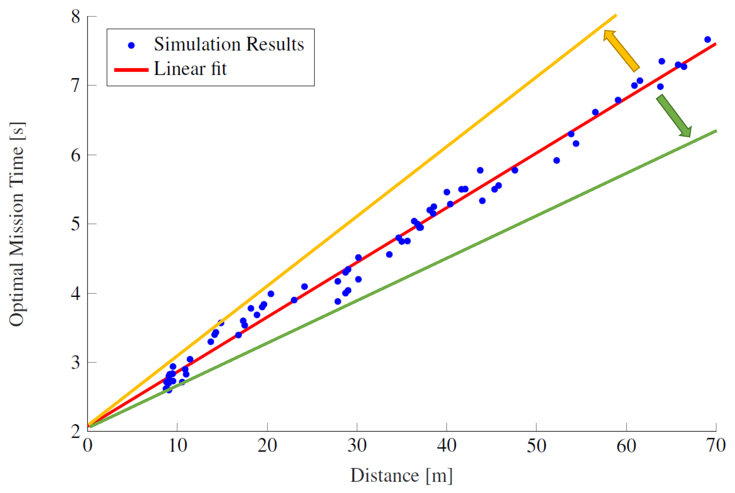
4.2.1. Optimal Mission-Time Setting

For a mission defined by initial and final positions $(x_0,y_0,z_0)$ and $(x_f,y_f,z_f)$, the Euclidean distance d is computed as $d=\sqrt{{(x_f-x_0)}^2+{(y_f-y_0)}^2+{(z_f-z_0)}^2}$. This distance serves as a crucial metric influencing the optimal travel time $t_{\mathrm{opt}}$, a parameter intricately tied to energy consumption. The relationship between $t_{\mathrm{opt}}$ and d is graphically depicted in Figure 2, showcasing the interplay between mission distance and the UAV’s physical constraints, such as the maximum rotation speed of the motors. The specific parameters for the chosen UAV will be provided in Section 6. Adjusting the UAV characteristics introduces shifts in the linear fit, represented by an upward (orange straight line) or downward (green straight line) trend in Figure 2. This adjustment depends on whether a lower- or higher-performing UAV is utilized. It is advisable to gradually increase the intercept of the line while maintaining a margin, to avoid operating at the limits of actuator saturation. This strategic approach ensures optimal performance within the specified UAV characteristics.

4.2.2. Optimal Trajectory References

Given $t_{\mathrm{opt}}$, the solution to the optimal control problem outlined in Section 4.1 is scrutinized, to derive sub-optimal profiles for position and speed along the three reference axes. Figure 3 showcases the optimal trends for positions and velocities across four randomly selected maneuvers from a diverse set of simulated missions. The first column illustrates the trends of $x_{\mathrm{opt}}$, $y_{\mathrm{opt}}$, and $z_{\mathrm{opt}}$, while the second column presents ${\dot{x}}_{\mathrm{opt}}$, ${\dot{y}}_{\mathrm{opt}}$, and ${\dot{z}}_{\mathrm{opt}}$. The missions are initialized from the origin for generality, and the final position points are as follows: $[6,6,3]$, $[8,6,10]$, $[17,8,5]$, $[10,10,10]$. Each mission exhibits a distinct optimal time, intricately tied to the distance and approximated through the regression line calculated in Section 4.2.1. For each mission, the optimal reference velocities are approximated with parabolas, and their features are influenced by the optimal mission time ($t_{\mathrm{opt}}$), the mission distance (d), and the final positions. This approach allows the generation of near-optimal energetic reference trajectories for velocity along the three axes without solving the optimal control problem repeatedly. Parabolic approximations for optimal-energetic-velocity profiles are defined for each axis:

$$k_{\mathrm{ref}}\left(t\right)=a{t}^2+bt+c,t\in [0,t_{\mathrm{opt}}].$$

(19)

In this expression, the coefficients a, b, c and the tuning parameter $k_M$ determine the shape of the parabola, with $k_0$ being the starting point and $k_{\mathrm{ref}}$ representing the reference velocity for the specific axis considered. The tuning parameter $k_M$ influences the maximum of the parabola and is computed based on the final value $k_f$ of the considered axis and $k_{\mathrm{opt}}\left(d\right)$, a tuning parameter of the reference trajectories generator that depends on d:

$$k_M=k_{\mathrm{opt}}\left(d\right)k_f.$$

(20)

Following the parabolic approximations of the optimal reference velocities along the three axes, the next step involves their integration, to compute the position reference trajectories. This seamless integration ensures a cohesive and synchronized representation of the optimal path for the UAV. Given the initial condition ${\gamma }_{\mathrm{ref}}\left(0\right)={\gamma }_0$ with ${\gamma }_{\mathrm{ref}}\in \{x_{\mathrm{ref}},y_{\mathrm{ref}},z_{\mathrm{ref}}\}$, we obtain

$${\gamma }_{\mathrm{ref}}\left(t\right)=\frac{a}{3}{t}^3+\frac{b}{2}{t}^2-k_{0}t+{\gamma }_{\mathrm{ref}}\left(0\right),$$

(21)

Which constitutes the approximated optimal positions trajectory. Analyzing the patterns in optimal position reference trajectories indicates that cubic curves are effective in approximating these functions. Similarly, the optimal energetic yaw-rate trajectory and its derivative can be calculated and approximated using a cubic function and a parabola, respectively. In summary, the generation of near-optimal energetic reference trajectories becomes feasible without the need to solve any optimal control problem, offering instant tracking possibilities for positions, yaw rate, and their derivatives.

5. Hierarchical Real–Time Control

Reiterating, the (open-loop) optimal control outlined in Section 4.1 is computed offline, serving the exclusive purpose of generating energetic reference trajectories and benchmarking controller performance. For UAV control, a nonlinear-feedback-control approach, derived from the classical hierarchical control elucidated in [37], is employed instead. This approach ensures real-time adaptability and responsiveness in guiding the UAV along its trajectory. The controller is implemented in a digital mode by maintaining the virtual control functions $u_z$, $u_{\varphi }$, $u_{\theta }$, $u_{\psi }$ in (4) constant within each time interval $[t_i,t_{i+1})$, where $t_{i+1}-t_i=\Delta t$ for $i=0,\cdots ,i_{max}-1$ and $t_{i_{max}}=t_f$. This discrete-time approach ensures stability and facilitates precise control within specified intervals, contributing to the overall effectiveness of the UAV control system. To streamline the design process, the motor dynamics ${\omega }_i$, $i=1,2,3,4$ are initially ignored in the control design. These dynamics are introduced in the final step through digital approximation and Equation (5). The initial focus is on establishing the desired closed-loop dynamics for the vertical position and velocity. This simplification aids in isolating and addressing specific control aspects before incorporating the complexities introduced by the motor dynamics:

$$\ddot{z}\left(t\right)={\ddot{z}}_{\mathrm{ref}}\left(t\right)-k_{pz}(z\left(t\right)-z_{\mathrm{ref}}\left(t\right))-k_{dz}(\dot{z}\left(t\right)-{\dot{z}}_{\mathrm{ref}}\left(t\right)),$$

(22)

with $k_{pz},k_{dz}>0$, $z_{\mathrm{ref}}\left(t\right)=x_5^{★}\left(t\right)$, ${\dot{z}}_{\mathrm{ref}}\left(t\right)=x_6^{★}\left(t\right)$, and $x^{★}$ being the known optimal trajectory (see Section 4.1), and where ${\ddot{z}}_{\mathrm{ref}}\left(t\right)$ can be computed by numerical differentiation. By comparing (22) to the third equation in (4), one obtains the linearizing controller,

$$u_z\left(t\right)=m\frac{{\ddot{z}}_{\mathrm{ref}}\left(t\right)-k_{pz}{e}_z\left(t\right)-k_{dz}{\dot{e}}_z\left(t\right)+g}{cos\theta cos\varphi },$$

(23)

having defined $e_z\left(t\right)=z\left(t\right)-z_{\mathrm{ref}}\left(t\right)$. By choosing a linearizing controller that incorporates gains $k_{pz}$ and $k_{dz}$ for the vertical position and velocity pair $(z,\dot{z})$, it is observed that this selection linearizes this pair into a chain of integrators. The gains $k_{pz}$ and $k_{dz}$ contribute to exponentially stable error dynamics. Following a similar procedure, the linearizing controller is applied, to achieve the desired closed-loop dynamics for the yaw position and velocity. This strategic approach ensures stability and enforces the desired dynamics in the controlled variables:

$$u_{\psi }\left(t\right)=\ddot{\psi }\left(t\right)={\ddot{\psi }}_{\mathrm{ref}}\left(t\right)-k_{p\psi }{e}_{\psi }\left(t\right)-k_{d\psi }{\dot{e}}_{\psi }\left(t\right),$$

(24)

with $k_{p\psi },k_{d\psi }>0$, having defined $e_{\psi }\left(t\right)=\psi \left(t\right)-{\psi }_{\mathrm{ref}}\left(t\right)$, ${\psi }_{\mathrm{ref}}\left(t\right)=x_{11}^{★}\left(t\right)$, ${\dot{\psi }}_{\mathrm{ref}}\left(t\right)=x_{12}^{★}\left(t\right)$. Substituting (23) into (4), and omitting the time dependencies, one obtains

$$\begin{array}{cc}\hfill \ddot{x}& =\left(\frac{tan\varphi sin\psi }{cos\theta }+cos\psi tan\theta \right)({\ddot{z}}_{\mathrm{ref}}-k_{pz}{e}_z-k_{dz}{\dot{e}}_z+g)\hfill \\ \hfill \ddot{y}& =\left(tan\theta sin\psi -\frac{cos\psi tan\varphi }{cos\theta }\right)({\ddot{z}}_{\mathrm{ref}}-k_{pz}{e}_z-k_{dz}{\dot{e}}_z+g).\hfill \end{array}$$

(25)

The hierarchical-control approach employs high gains $k_{pz}$, $k_{dz}$, $k_{p\psi }$, $k_{d\psi }$ to impose rapid yaw and vertical dynamics. By choosing sufficiently high gains, the position and velocity errors for yaw and vertical dynamics rapidly converge to zero within each interval $[t_i,t_{i+1})$. This allows for a simplified approximation in which these errors are effectively reduced to zero during each interval, facilitating efficient control implementation:

$$\begin{array}{cc}\hfill \ddot{x}& =\left(\frac{tan\varphi sin\psi }{cos\theta }+cos\psi tan\theta \right)({\ddot{z}}_{\mathrm{ref}}+g)\hfill \end{array}$$

(26)

$$\begin{array}{cc}\hfill \ddot{y}& =\left(tan\theta sin\psi -\frac{cos\psi tan\varphi }{cos\theta }\right)({\ddot{z}}_{\mathrm{ref}}+g).\hfill \end{array}$$

(27)

The desired closed–loop dynamics for the $(x,y)$ positions and velocities is expressed by

$$\begin{array}{cc}\hfill \ddot{x}\left(t\right)& ={\ddot{x}}_{\mathrm{ref}}\left(t\right)-k_{px}{e}_x\left(t\right)-k_{dx}{\dot{e}}_x\left(t\right)\hfill \end{array}$$

(28)

$$\begin{array}{cc}\hfill \ddot{y}\left(t\right)& ={\ddot{y}}_{\mathrm{ref}}\left(t\right)-k_{py}{e}_y\left(t\right)-k_{dy}{\dot{e}}_y\left(t\right),\hfill \end{array}$$

(29)

with $k_{px},k_{dx},k_{py},k_{dy}>0$, $e_x\left(t\right)=x\left(t\right)-x_{\mathrm{ref}}\left(t\right)$, $e_y\left(t\right)=y\left(t\right)-y_{\mathrm{ref}}\left(t\right)$, $x_{\mathrm{ref}}\left(t\right)=x_1^{★}\left(t\right)$, ${\dot{x}}_{\mathrm{ref}}\left(t\right)=x_2^{★}\left(t\right)$, $y_{\mathrm{ref}}\left(t\right)=x_3^{★}\left(t\right)$, ${\dot{y}}_{\mathrm{ref}}\left(t\right)=x_4^{★}\left(t\right)$. By comparing (26) and (27) to (28) and (29), and by utilizing the small angle condition $cos\theta \approx 1$ in the denominator of (26), explicit approximate expressions for the reference angles $(\varphi ,\theta )$ are derived. These expressions effectively impose the desired dynamics in (28) and (29). This analytical approach enhances the understanding and implementation of the desired control dynamics for the UAV:

$$\begin{array}{cc}\hfill {\varphi }_{\mathrm{ref}}& =arctan\left(sin\theta tan\psi -\frac{cos\theta ({\ddot{y}}_{\mathrm{ref}}-k_{py}{e}_y-k_{dy}{\dot{e}}_y)}{({\ddot{z}}_{\mathrm{ref}}+g)cos\psi }\right)\hfill \end{array}$$

(30)

$$\begin{array}{cc}\hfill {\theta }_{\mathrm{ref}}& =arctan\left(\frac{{\ddot{x}}_{\mathrm{ref}}-k_{px}{e}_x-k_{dx}{\dot{e}}_x}{({\ddot{z}}_{\mathrm{ref}}+g)cos\psi }-tan\varphi tan\psi \right)\hfill \end{array}$$

(31)

To ensure the rapid convergence of the $(\varphi ,\theta )$ dynamics to the reference values $({\varphi }_{\mathrm{ref}},{\theta }_{\mathrm{ref}})$, additional constraints are imposed. These constraints contribute to the overall stability and precision of the control system, ensuring that the UAV quickly converges to the desired orientation:

$$\begin{array}{cc}\hfill u_{\varphi }\left(t\right)& =\ddot{\varphi }\left(t\right)=-k_{p\varphi }(\varphi \left(t\right)-{\varphi }_{\mathrm{ref}})-k_{d\varphi }\dot{\varphi }\left(t\right)\hfill \end{array}$$

(32)

$$\begin{array}{cc}\hfill u_{\theta }\left(t\right)& =\ddot{\theta }\left(t\right)=-k_{p\theta }(\theta \left(t\right)-{\theta }_{\mathrm{ref}})-k_{d\theta }\dot{\theta }\left(t\right),\hfill \end{array}$$

(33)

with sufficiently high gains $k_{p\varphi },k_{d\varphi },k_{p\theta },k_{d\theta }>0$. As pointed out at the beginning of this section, a digital implementation of the control laws $u_z$, $u_{\psi }$, $u_{\varphi }$, $u_{\theta }$ in (22) and (23), (32) and (33) consists in sampling the right-hand sides of these equations at each time $t_i$ and holding the inputs $u_z\left(t_i\right)$, $u_{\psi }\left(t_i\right)$, $u_{\varphi }\left(t_i\right)$, $u_{\theta }\left(t_i\right)$ within each interval $[t_i,t_{i+1})$. As a terminal step, the computation of concrete inputs ${\alpha }_j\left(t_i\right)$, $j=1,2,3,4$, i.e., the four motor accelerations, to plug into Equation (14) is required. To this end, from the knowledge of the angle velocities $\varphi \left(t_i\right)$, $\theta \left(t_i\right)$, $\psi \left(t_i\right)$ and the virtual inputs $u_z\left(t_i\right)$, $u_{\psi }\left(t_i\right)$, $u_{\varphi }\left(t_i\right)$, $u_{\theta }\left(t_i\right)$, we progress with the partial inversion of (5) to calculate the demanded motor velocities ${\omega }_j\left(t_i\right)$, $j=1,2,3,4$, so that the digital actuations are obtained, by first-order discretization of the last equations in (14), as

$${\alpha }_j\left(t_i\right)=\frac{{\omega }_j\left(t_i\right)-{\omega }_j\left(t_{i-1}\right)}{\Delta t}j=1,2,3,4.$$

(34)

6. Simulation Results

This section delves into the performance evaluation of the proposed controller. The simulation environment is initially described, followed by the presentation of the results obtained by the controller on the Simcenter Amesim Drone model. The section concludes with final considerations on the energy aspects, providing a comprehensive assessment of the controller’s effectiveness and impact on UAV dynamics.

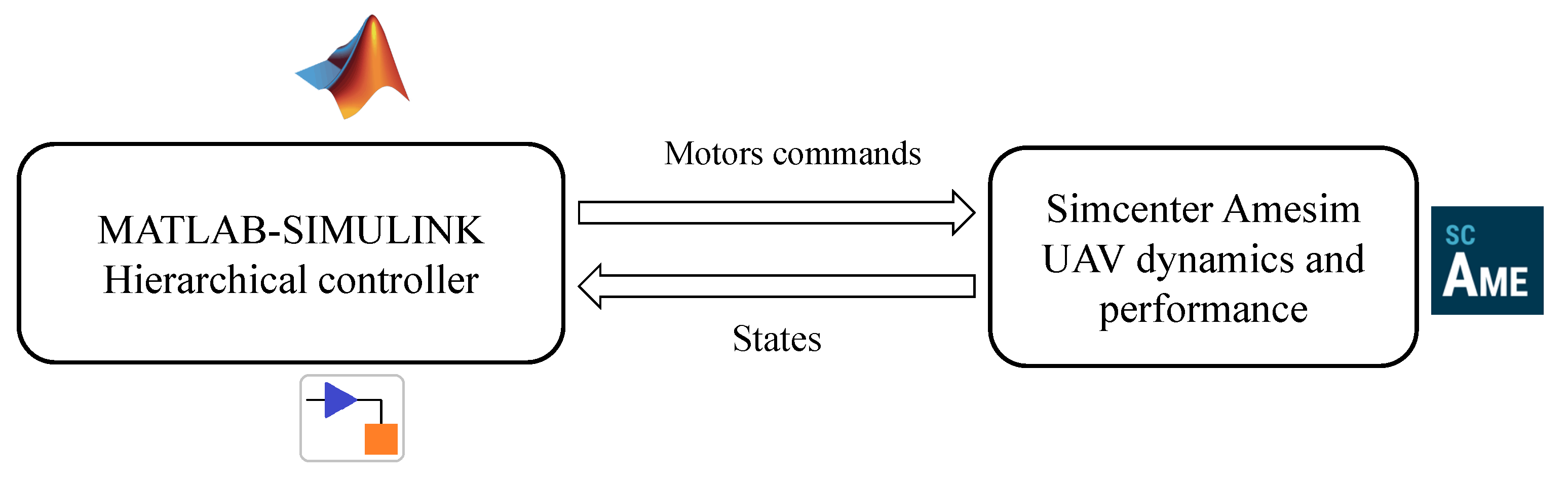
6.1. Co-Simulation Environment with Matlab and Simcenter Amesim

The interest in introducing numerical simulation in this study lies in the possibility of assessing the controllers’ behavior when integrated with a plant model or virtual prototype of the UAV. System simulation is particularly convenient for this purpose as it enables the creation of a dynamic and multi-physics performance model of the UAV with a fidelity sufficiently high to effectively support the continuous development of sophisticated control algorithms, including their virtual verification and validation (V&V) (see [42]). The tools selected for this analysis were Matlab Simulink for the modeling and simulation of the controllers and Simcenter Amesim as the dynamic, multi-physics system simulation tool (see [43] for more details). Edited by Siemens Digital Industries Software, Simcenter Amesim provides off-the-shelf components available in libraries, covering several physical (fluids, mechanical, electrical, thermal) and application (aerospace, automotive, gas turbines) domains. These are well suited to modeling different subsystems of the UAV, such as energy storage (e.g., lithium-ion batteries), propulsion (e.g., electric motors and propellers), and flight dynamics. As discussed in [42], models of UAV subsystems built with this tool have been favorably compared against experimental data provided by manufacturers or found in the scientific literature. This co-simulation approach leverages the best capabilities of the two tools selected in their respective fields, allowing to investigate the behavior of the controllers under the large variety of operating conditions to be expected during the UAV mission, including failures.

The Simcenter Amesim plant model is more complex with respect to the reference mathematical model considered for the design of the controller presented in Section 2, as it contains additional phenomena as well as time-varying parameters. For this reason, it is also regarded as a valid test bed for the controller. Consequently, the parameters used in the model-based controller had to be identified, as done in Section 3. For example, the propellers’ aerodynamic properties, such as the thrust and drag coefficients, play an important role in the design of the controller. Several studies have shown that these coefficients depend on the propellers’ operating conditions. Both in the physical models used in the advanced and realistic simulator described in this paper (see [42]) and in experimental studies they are determined by multi-variable functions (see [44,45]) depending on the propeller orientation, angular velocity, and total velocity as well as the geometric characteristics.

The results presented in Section 6.2 have been simulated in a co-simulation framework whose purpose is to couple the physical Simcenter Amesim model, representative of the UAV and its subsystems performance, to the hierarchical control algorithm designed in Matlab Simulink. The approach used in this paper, conceptualized in Figure 4, connects Matlab Simulink through a dedicated interface with Simcenter tools.

In this study, these parameters were identified statically for the controller design, even though they were time-varying during the simulation. To account for this simplification, and increase the controllers robustness, variations in the propulsion level were also considered in the disturbance term.

The drone simulation parameters used in the model-based design controller are presented in

Table 1. Nominal quadrotor parameters.

m	Mass of the Airframe	5 kg
l	Distance of the center of mass to the rotor shaft	0.3 m
$J_1$	Inertia in the x-axis	0.011521 kg $·$ ${\mathrm{m}}^2$
$J_2$	Inertia in the y-axis	0.0362132   kg $·$ ${\mathrm{m}}^2$
$J_3$	Inertia in the z-axis	0.029142  kg $·$ ${\mathrm{m}}^2$
$J_p$	Inertia of the propellers	0.0003  kg $·$ ${\mathrm{m}}^2$
g	Gravity acceleration	9.81   m $·$ $s^{-2}$
b	Trust factor	$4.5625·{10}^{-5}$  N $·s^2·$ ${\mathrm{rad}}^{-2}$
c	Drag factor	$1.375·{10}^{-5}$ N ${\mathrm{s}}^2·$ ${\mathrm{rad}}^{-2}·$ m

.

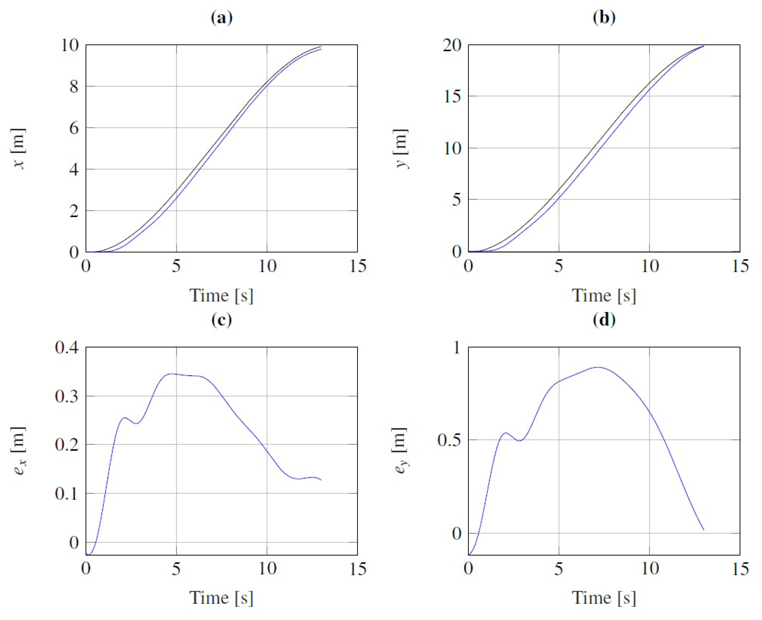
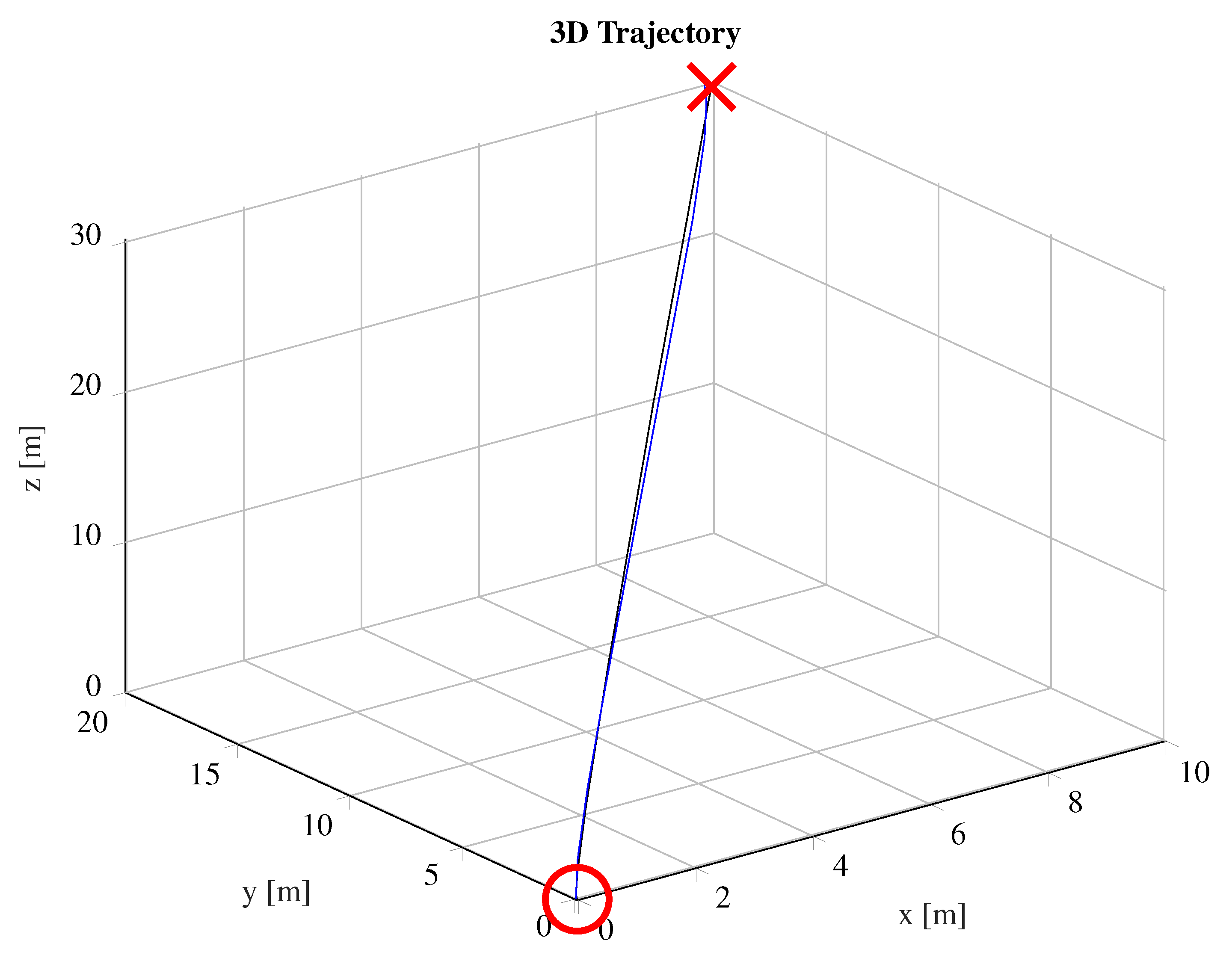
6.2. Simulation Results in Simulink and Simcenter Amesim Co-Simulation Platform

In the test mission shown, we considered rest-to-rest maneuvers of the Simcenter Amesim quadrotor with an initial state $\left[xyz\psi \right]=\left[0000\right]$ and $\left[xyz\psi \right]=[102030\pi /4]$ as the desired final state. In fact, we assumed zero linear and angular velocity of the UAV at the boundary states, with zero body orientation at time $t=0$. The gains values of the controller used in the simulations shown are reported in the

Table 2. Parameters of Controller.

$k_{px}=k_{py}=4$	$k_{dx}=k_{dy}=1$	$k_{pz}=50$	$k_{dz}=5$
$k_{p\theta }=k_{p\varphi }=k_{p\psi }=5$	$k_{d\theta }=0.5$	$k_{d\varphi }=0.5$	$k_{d\psi }=0.5$

. Figure 5, Figure 6, Figure 7, Figure 8 and Figure 9 show the main profiles that characterize the considered simulation. Figure 5 shows the references and controlled Simcenter Amesim drone position, both along the x-axis (a) and along the y-axis (b), while in (c) and (d) the subplots refer to the respective errors. Due to the unmodeled dynamics and the uncertainty of some parameters, the error is not exactly negligible, but it is still limited.

Figure 6 shows the references and controlled drone position along the z-axis (a) and with respect to the yaw angle (b). Sub-figures (c) and (d) show the respective errors, which are limited. At the level of the desired three-dimensional trajectory, shown in Figure 7, it is tracked well and the error that is committed is negligible, considering the complexity of the model that one tries to control.

Figure 8 shows the angular speeds of the four drone propellers, which never reached saturation (set at approximately 6.400 rpm), indicating that the simulation time chosen at the reference generation level according to the logic obtained in Section 3 was correct. Finally, Figure 9 shows the state of charge of the drone battery: approximately $1.2\%$ was consumed in the considered maneuver.

Table 3. Comparison of optimal control (OC), SMC (simplified model control), and SAC (Simcenter Amesim control) to rule-based energetic references generator over various heterogeneous missions. EC stands for energy consumption J. BC stands for battery consumption.

	EC J			BC
Final Point	OC	SMC	SAC	OC	SMC	SAC
[10,20,30]	100	101.52	101.43	100	101.31	101.27
[12,10,−40]	100	102.23	102.3	100	102.09	102.14
[8,10,6]	100	101.1	100.71	100	100.92	100.54
[−30,40,50]	100	102.3	101.9	100	102.11	101.78
[20,−20,−40]	100	102.17	102.02	102	102.21	101.95

presents a comparison of the energy consumptions between the optimal control (OC), the hierarchical control applied to the simplified model (SM), and the hierarchical control applied to the Simcenter Amesim model (AM). The comparison is made in terms of the chosen cost functional J defined in Equation (8) and the state of charge (SOC) at the end of the selected maneuvers. Remarkably, the proposed rule-based strategy with hierarchical control closely aligns with the optimal open-loop solution in both energy and battery terms. Additionally, the values of the two performance criteria are consistently very close for the controller applied to both the simplified model and the Simcenter Amesim model, suggesting that the chosen cost functional J serves as an effective measure of real battery consumption. The proposed control scheme exhibits notable strength, in terms of computational efficiency. Leveraging linear interpolation and algebraic operations, it achieves quicker computation compared to the optimal strategy, where a minimization process is necessary. However, the optimal control strategy demands less calibration and offers ease of tuning for various missions or different UAVs. This trade-off highlights the efficiency and adaptability aspects of the proposed control approach, catering to diverse application scenarios and mission requirements.

7. Conclusions

The solution to the quadrotor mission control problem, aiming for the minimum achievable energy consumption along a mission, can be addressed through the optimal-control theory. However, implementing this approach onboard in real time poses challenges, due to limited computational and memory resources. On the other hand, a rule-based approach is better suited to online implementation, even though it necessitates a demanding calibration process. The strategy explored in this work involves analyzing decisions made by the optimal-control theory, to identify common patterns in optimal travel mission time and reference generation. The calibration parameters in the reference generator need to be tuned, to ensure that rule-based references closely match optimal trajectories. The hierarchical controller designed for this purpose, which effectively tracks reference trajectories and energy consumption, both in terms of the functional defined in the optimal control problem and battery consumption, closely aligns with the optimal solution. It is crucial to emphasize that the reference generator and optimal mission time are contingent on the type of UAV and its specific characteristics. Any variations in these parameters would require a redesign. A prospective investigation could involve observing the different trajectories chosen by the optimal controller as the drone parameters, energy sources, and architecture undergo changes. The proposed controller’s results were validated through numerical experiments, and comparisons were made in terms of trajectory tracking, energy performance index, and battery consumption using the Simcenter Amesim physical model in a co-simulation framework with Matlab-Simulink. This comprehensive approach provided insights into the practicality and effectiveness of the proposed rule-based strategy in real-world UAV applications.

In future investigations, a significant enhancement will entail integrating a disturbance estimator into the controller, similar to the approach presented in [46]. While the current study focuses on the energy and control aspects within a commercial simulator, external disturbances—such as wind—were not taken into account. The inclusion of a disturbance estimator is intended to improve the robustness of the control action, reducing errors attributed to non-modeled dynamics and time-varying parameters. This measure is essential, to ensure the efficacy and dependability of the control strategy in real-world scenarios, where external factors can influence the performance of UAVs.

References

1. Mathews, A.J.; Singh, K.; Cummings, A.R.; Rogers, S.R. Fundamental practices for drone remote sensing research across disciplines. Drone Syst. Appl. 2023, 11, 1–22. [Google Scholar] [CrossRef]
2. Santoso, F.; Garratt, M.A.; Anavatti, S.G. State-of-the-art intelligent flight control systems in unmanned aerial vehicles. IEEE Trans. Autom. Sci. Eng. 2018, 15, 613–627. [Google Scholar] [CrossRef]
3. DDC: Drone Delivery Canada. Available online: https://dronedeliverycanada.com/ (accessed on 17 August 2023).
4. Wall Street Journal, Google Drones Can Already Deliver You Coffee In Australia. Available online: www.youtube.com/watch?v=prhDrfUgpB0 (accessed on 6 April 2019).
5. Zraick, K. Like ‘Uber for Organs’: Drone Delivers Kidney to Maryland Woman. The New York Times. Available online: www.nytimes.com/2019/04/30/health/drone-delivers-kidney.html (accessed on 17 August 2023).
6. Estevez, J.; Lopez-Guede, J.M.; Grana, M. Quasi-stationary state transportation of a hose with quadrotors. Robot. Auton. Syst. 2015, 63, 187–194. [Google Scholar] [CrossRef]
7. Post, S. Drones: A Vision Has Become Reality. Available online: http://www.swisspost.ch/drones (accessed on 17 August 2023).
8. Stolaroff, J.K.; Samaras, C.; O’Neill, E.R.; Lubers, A.; Mitchell, A.S.; Ceperley, D. Energy use and life cycle greenhouse gas emissions of drones for commercial package delivery. Nat. Commun. 2018, 9, 409. [Google Scholar] [CrossRef] [PubMed]
9. Jensen-Nau, K.R.; Hermans, T.; Leang, K.K. Near-optimal area-coverage path planning of energy-constrained aerial robots with application in autonomous environmental monitoring. IEEE Trans. Autom. Sci. Eng. 2021, 18, 1453–1468. [Google Scholar] [CrossRef]
10. Lin, J.; Wang, Y.; Miao, Z.; Wang, H.; Fierro, R. Robust image-based landing control of a quadrotor on an unpredictable moving vehicle using circle features. IEEE Trans. Autom. Sci. Eng. 2023, 20, 1429–1440. [Google Scholar] [CrossRef]
11. Bresciani, T. Modelling, Identification and Control of a Quadrotor Helicopter. Master’s Thesis, Department of Automatic Control, Lund University, Lund, Sweden, 2008. [Google Scholar]
12. Swieringa, K.A.; Hanson, C.B.; Richardson, J.R.; White, J.D.; Hasan, Z.; Qian, E.; Girard, A. Autonomous battery swapping system for small–Scale helicopters. In Proceedings of the 2010 IEEE International Conference on Robotics and Automation, Anchorage, AL, USA, 3–8 May 2010; pp. 3335–3340. [Google Scholar] [CrossRef]
13. Leonard, J.; Savvaris, A.; Tsourdos, A. Energy management in swarm of unmanned aerial vehicles. J. Intell. Robot. Syst. 2014, 74, 233–250. [Google Scholar] [CrossRef]
14. Junaid, A.B.; Konoiko, A.; Zweiri, Y.; Sahinkaya, M.; Seneviratne, L. Autonomous wireless selfcharging for multi-rotor unmanned aerial vehicles. Energies 2017, 10, 803. [Google Scholar] [CrossRef]
15. Campi, T.; Cruciani, S.; Feliziani, M. Wireless power transfer technology applied to an autonomous electric uav with a small secondary coil. Energies 2018, 11, 352. [Google Scholar] [CrossRef]
16. Kumar, V.; Michael, N. Opportunities and challenges with autonomous micro aerial vehicles. Int. J. Robot. Res. 2012, 31, 1279–1291. [Google Scholar] [CrossRef]
17. Abdilla, A.; Richards, A.; Burrow, S. Power and endurance modelling of battery-powered rotorcraft. In Proceedings of the IEEE International Conference on Intelligent Robots and Systems, Hamburg, Germany, 28 September–2 October 2015; pp. 675–680. [Google Scholar] [CrossRef]
18. Morton, S.; Papanikolopoulos, N. A small hybrid ground-air vehicle concept. In Proceedings of the IEEE/RSJ International Conference on Intelligent Robots and Systems (IROS), Vancouver, BC, Canada, 1–5 October 2017; pp. 5149–5154. [Google Scholar] [CrossRef]
19. Economou, J.; Kladis, G.; Tsourdos, A.; White, B. UAV optimum energy assignment using Dijkstra’s algorithm. In Proceedings of the European Control Conference (ECC), Kos, Greece, 2–5 July 2007; pp. 287–292. [Google Scholar] [CrossRef]
20. Carvajal, C.P.; Andaluz, V.H.; Roberti, F.; Carelli, R. Path-following control for aerial manipulators robots with priority on energy saving. Control. Eng. Pract. 2023, 131, 105401. [Google Scholar] [CrossRef]
21. Mohiuddin, A.; Taha, T.; Zweiri, Y.; Gan, D. Dual-uav payload transportation using optimized velocity profiles via real-time dynamic programming. Drones 2023, 7, 171. [Google Scholar] [CrossRef]
22. Levermore, T.; Sahinkaya, M.N.; Zweiri, Y.; Neaves, B. Real-time velocity optimization to minimize energy use in passenger vehicles. Energies 2017, 10, 30. [Google Scholar] [CrossRef]
23. Rossi, R.; Santamaria-Navarro, A.; Andrade-Cetto, J.; Rocco, P. Trajectory generation for unmanned aerial manipulators through quadratic programming. IEEE Robot. Autom. Lett. 2017, 2, 389–396. [Google Scholar] [CrossRef]
24. Kreciglowa, N.; Karydis, K.; Kumar, V. Energy efficiency of trajectory generation methods for stop-and-go aerial robot navigation. In Proceedings of the International Conference on Unmanned Aircraft Systems (ICUAS), Miami, FL, USA, 13–16 June 2017; pp. 656–662. [Google Scholar] [CrossRef]
25. Jacewicz, M.; Zugaj, M.; Glebocki, R.; Bibik, P. Quadrotor model for energy consumption analysis. Energies 2022, 15, 7136. [Google Scholar] [CrossRef]
26. Chodnicki, M.; Siemiatkowska, B.; Stecz, W.; Stepien, S. Energy efficient uav flight control method in an environment with obstacles and gusts of wind. Energies 2022, 15, 3730. [Google Scholar] [CrossRef]
27. Morbidi, F.; Cano, R.; Lara, D. Minimum-energy path generation for a quadrotor UAV. In Proceedings of the IEEE International Conference on Robotics and Automation (ICRA), Stockholm, Sweden, 16–21 May 2016; pp. 1492–1498. [Google Scholar] [CrossRef]
28. Zhou, H.; Xiong, H.L.; Liu, Y.; Tan, N.D.; Chen, L. Trajectory planning algorithm of uav based on system positioning accuracy constraints. Electronics 2020, 9, 250. [Google Scholar] [CrossRef]
29. Yu, G.; Cabecinhas, D.; Cunha, R.; Silvestre, C. Quadrotor trajectory generation and tracking for aggressive maneuvers with attitude constraints. IFAC-PapersOnLine. 2019, 52, 55–60. [Google Scholar] [CrossRef]
30. Schacht-Rodriguez, R.; Ponsart, J.C.; Garcia-Beltran, C.D.; Astorga-Zaragoza, C.M.; Theilliol, D.; Zhang, Y. Path planning generation algorithm for a class of uav multirotor based on state of health of lithium polymer battery. J. Intell. Robot. Syst. 2018, 91, 115–131. [Google Scholar] [CrossRef]
31. Wu, M.; Chen, W.; Tian, X. Optimal Energy Consumption Path Planning for Quadrotor UAV Transmission Tower Inspection Based on Simulated Annealing Algorithm. Energies 2022, 15, 8036. [Google Scholar] [CrossRef]
32. Jiang, B.; Li, B.; Zhou, W.; Lo, L.-Y.; Chen, C.-K.; Wen, C.-Y. Neural Network Based Model Predictive Control for a Quadrotor UAV. Aerospace 2022, 9, 460. [Google Scholar] [CrossRef]
33. Giernacki, W. Minimum Energy Control of Quadrotor UAV: Synthesis and Performance Analysis of Control System with Neurobiologically Inspired Intelligent Controller (BELBIC). Energies 2022, 15, 7566. [Google Scholar] [CrossRef]
34. Bianchi, D.; Rolando, L.; Serrao, L.; Onori, S.; Rizzoni, G.; Al-Khayat, N.; Hsieh, T.; Kang, P.T. Layered control strategies for hybrid electric vehicles based on optimal control. Int. J. Electr. Hybrid Veh. (IJEHV) 2011, 3, 191–217. [Google Scholar] [CrossRef]
35. Gieras, J.F. Permanent Magnet Motor Technology: Design and Applications; CRC Press, Taylor and Francis Group: Boca Raton, FL, USA, 2009. [Google Scholar]
36. Bouabdallah, S.; Murrieri, P.; Siegwart, R. Towards autonomous indoor micro vtol. Auton. Robot. 2005, 18, 171–183. [Google Scholar] [CrossRef]
37. Carrillo, L.R.; Lopez, A.E.; Lozano, R.; Pegard, C. Quad Rotorcraft Control: Vision-Based Hovering and Navigation; Springer: London, UK, 2013. [Google Scholar]
38. Lua, C.A.; Garcia, C.C.V.; Di Gennaro, S.; Castillo–Toledo, B.; Morales, M.E.S. Real–time hovering control of unmanned aerial vehicles. Math. Probl. Eng. 2020, 2020, 2314356. [Google Scholar] [CrossRef]
39. Mendoza, L.F.M.; Bonilla, J.T.G.; Garcia-Torales, G.; Lua, C.A.; Di Gennaro, S. Visual Sensor System Applied to Trajectory Generation for UAVs. In Proceedings of the IEEE International Autumn Meeting on Power, Electronics and Computing (ROPEC), Ixtapa, Mexico, 9–11 November 2022. [Google Scholar] [CrossRef]
40. Li, Y.R.; Peng, C.C. Development of a full orientation flight robotics: Dynamics modeling, analysis, and control design. IEEE Access 2023, 11, 110234–110244. [Google Scholar] [CrossRef]
41. Jongerden, M.R.; Haverkort, B.R. Which battery model to use? IET Softw. 2012, 3, 445–457. [Google Scholar] [CrossRef]
42. Cappuzzo, F.; Dezobry, V.; Bianchi, D.; Di Gennaro, S. A Novel Co-simulation framework for Verification and Validation of GNC Algorithms for Autonomous UAV. In Proceedings of the Vertical Flight Society’s 78th Annual Forum & Technology Display, Fort Worth, TX, USA, 10–12 May 2022. [Google Scholar]
43. Siemens: Simcenter Amesim 2021.1 Reference Guide 2021. Available online: https://docs.plm.automation.siemens.com/content/amesim/17/help/en_US/quick_start_guide/references.html (accessed on 19 January 2024).
44. Nguyen, D.H.; Liu, Y.; Mori, K. Experimental study for aerodynamic performance of quadrotor helicopter. Trans. Jpn. Soc. Aeronaut. Space Sci. 2018, 61, 29–39. [Google Scholar] [CrossRef]
45. Six, D.; Briot, S.; Erskine, J.; Chriette, A. Identification of the propeller coefficients and dynamic parameters of a hovering quadrotor from flight data. IEEE Robot. Autom. Lett. 2020, 5, 1063–1070. [Google Scholar] [CrossRef]
46. Bianchi, D.; Di Gennaro, S.; Di Ferdinando, M.D.; Lua, C.A. Robust control of uav with disturbances and uncertainty estimation. Machines 2023, 11, 352. [Google Scholar] [CrossRef]
Figure 1. Electrical model of the brushless DC motor of a quadrotor UAV.
Drones 08 00029 g001
Figure 2. Battery-state-of-charge-(SOC) trajectory in Simcenter Amesim and in the simplified quadrotor model.
Drones 08 00029 g002
Figure 3. Dependence of the optimal mission time on distance d. In blue the optimal times as a function of the distance derived from the solution of the optimal control problem, and in red a linear approximation of the data. The orange and green straight lines correspond to shifts in the linear fit due to adjustments of the UAV characteristics.
Drones 08 00029 g003
Figure 4. Optimal trajectories reference for some selected test simulations with final position states equal to [ 6 6 3 ] , [ 8 6 10 ] , [ 17 8 5 ] , [ 10 10 10 ] : (a) Optimal position trends along the x-axis. (b) Optimal position trends along the y-axis. (c) Optimal position trends along the z-axis. (d) Optimal velocity trends along the x-axis. (e) Optimal velocity trends along the y-axis. (f) Optimal velocity trends along the z-axis.
Drones 08 00029 g004
Figure 5. The co-simulation framework.
Drones 08 00029 g005
Figure 6. (a) Longitudinal motion of the UAV: the reference x r e f (black) and the controlled x (blue). (b) Latitudinal motion of the UAV: the reference y r e f (black) and the controlled y (blue). (c) Longitudinal error motion of the controlled UAV (x-axis). (d) Latitudinal error motion of the controlled UAV (y-axis).
Drones 08 00029 g006
Figure 7. (a) Quadrotor’s altitude motion: the reference z r e f (black) and the controlled z (blue). (b) Quadrotor yaw angle: the reference ψ r e f (black) and the controlled ψ (blue). (c) Altitude error motion of the UAV (z-axis). (d) Yaw angle error of the controlled UAV.
Drones 08 00029 g007
Figure 8. 3D drone trajectory: reference (black), robust control (blue). The circle and the cross indicate, respectively, the starting and ending point of the 3D reference trajectory.
Drones 08 00029 g008
Figure 9. Propulsion angular velocities of the proposed controller: ω 1 (a), ω 2 (b), ω 3 (c), ω 4 (d).
Drones 08 00029 g009
Figure 10. SOC of the battery profile during considered simulation.
Drones 08 00029 g010