Article

Thermal Monitoring of an Internal Combustion Engine for Lightweight Fixed-Wing UAV Integrating PSO-Based Modelling with Condition-Based Extended Kalman Filter

by
Aleksander Suti
1,*,
Gianpietro Di Rito
1 and
Giuseppe Mattei
2
1
Department of Civil and Industrial Engineering, University of Pisa, Largo Lucio Lazzarino 2, 56122 Pisa, Italy
2
R&D Propulsion Team, Sky Eye Systems S.r.l., Via Grecia 52, 56021 Cascina, Italy
*
Author to whom correspondence should be addressed.
Drones 2024, 8(10), 531; https://doi.org/10.3390/drones8100531 (registering DOI)
Submission received: 19 August 2024 / Revised: 22 September 2024 / Accepted: 27 September 2024 / Published: 29 September 2024

Abstract

:
The internal combustion engines of long-endurance UAVs are optimized for cruises, so they are prone to overheating during climbs, when power requests increase. To counteract the phenomenon, step-climb maneuvering is typically operated, but the intermittent high-power requests generate repeated heating–cooling cycles, which, over multiple missions, may promote thermal fatigue, performance degradation, and failure. This paper deals with the development of a model-based monitoring of the cylinder head temperature of the two-stroke engine employed in a lightweight fixed-wing long-endurance UAV, which combines a 0D thermal model derived from physical first principles with an extended Kalman filter capable to estimate the head temperature under degraded conditions. The parameters of the dynamic model, referred to as nominal condition, are defined through a particle-swarm optimization, minimizing the mean square temperature error between simulated and experimental flight data (obtaining mean and peak errors lower than 3% and 10%, respectively). The validated model is used in a so-called condition-based extended Kalman filter, which differs from a conventional one for a correction term in section prediction, leveraged as degradation symptom, based on the deviation of the model-state derivative with respect to the actual measurement. The monitoring algorithm, being executable in real-time and capable of identifying incipient degradations of the thermal flow, demonstrates applicability for online diagnostics and predictive maintenance purposes.

1. Introduction

The internal combustion engines (ICEs) of long-endurance UAVs are optimized for cruise operations, to minimize fuel consumption at continuous low power regimes. This makes them prone to overheating during climb, when the power requests increase (in [1], it is pointed out that the temperature rise in the cylinder head of an UAV ICE can reach 1 °C per second). To avoid potential damages, step-climb maneuvering is typically operated, by alternating brief climbs and levelled flights, in order to maintain the cylinder head temperature (CHT) within allowable limits. Nevertheless, these intermittent high-power requests generate heating–cooling cycles, which, over multiple missions, may promote thermal fatigue [2], performance degradation [3], and failure. A model-based thermal monitoring of the ICE, capable of identifying incipient degradations and supporting unscheduled maintenance, could be crucial to counteract these concerns and increase system reliability and safety.
Literature proposes several thermal models for ICEs, which can be essentially categorized into n-Dimensional (nD, with n = 1, 2) and thermofluid dynamic models [4].
Thermofluid dynamic models are inherently unsteady and three-dimensional (3D); rely on conservation principles of mass, chemical species, momentum, and energy at any point within the engine cylinder; and utilize computation fluid dynamics (CFDs) to solve Navier–Stokes equations. On the other hand, nD models provide a simplified but effective representation of the thermodynamic process by solving mass and energy conservation along spatial gradients of pressure and temperature in n directions only.
CFD-based models are very accurate, but despite research efforts (in [5], an innovative method optimizing the computational costs for CFD simulations is proposed, by using the rate of heat release as a source term in the energy equation, thereby simplifying the combustion modelling), they are not real-time executable, and their use for monitoring purposes is currently unfeasible. Conversely, 0D or 1D models offer a good balance between accuracy and computational cost. In [6], a six-cylinder diesel engine is effectively modelled using a 1D approach, and Mauro et al. demonstrate that the heat release dynamics in an ICE can be well represented by a 0D model using the CHT as unique state variable [7].
Actually, although 0D models lack spatial gradients, they can be developed to address one or more specific zones in the combustion chamber, so that single-zone (SZ) or multiple-zone models are obtained [8]. Giglio et al. developed a nonlinear 0D Wiebe-based combustion model for a spark ignition (SI) ICE, which relates the mass-burned fraction with the crank angle, demonstrating its effectiveness with respect to a turbulent entrainment combustion model embedded in a 1D simulation model of the engine [9]. In [10], a 0D model is used to predict the heat release rate in an SI ICE, taking into account the geometry of the combustion chamber and the turbulence intensity, with good agreement with experimental data. Payri et al. [11] developed a 0D-SZ model that includes heat transfer with chamber walls, blow-by leakage, fuel injection, engine deformations, and instantaneous changes in gas properties. In [12], a 0D model is used to evaluate the effect of atmospheric conditions at different altitudes, confirming that altitude reduces the combustion efficiency and the power output. It is worth noting that, despite the extensive collection of thermal models related to ICEs for automotive and naval applications, the literature is poor if aircrafts and UAVs are concerned. In these problems, heat transfer is significantly impacted by altitude, which varies environmental temperature and density, as well as by the variations of the vehicle speed.
Once a representative thermodynamic model is obtained, a common approach to engine monitoring is to apply a Kalman Filter (KF) estimator [13]. In [14], a self-tuning on-board real-time model for health parameter estimation based on Linear Kalman Filter (LKF) is presented. The work employs a metaheuristic search optimization algorithm to generate a subset of health parameters that facilitates KF-based estimation. Effectively used for gas turbine health assessment and performance prognosis, the method tested in simulations on a turbofan engine demonstrates good efficiency in estimating health parameters coupled linearly with the errors. To decrease the estimation errors coupled with nonlinearities, Simon [15] presented a comparison between LKF and two nonlinear KF-based techniques known as the Extended Kalman Filter (EKF) and the Unscented Kalman filter (UKF) for the purpose of engine-health monitoring. The EKF linearizes the system around an estimate of the current mean and covariance, making it suitable for some nonlinear applications. However, in systems with significant nonlinear characteristics, the EKF may perform poorly. In contrast, the UKF can enhance model accuracy by employing deterministic sampling to derive new estimates for the mean and covariance. The study concludes that since the EKF necessitates an accurate model of engine dynamics’ nonlinearities, the UKF may not be justified due to its added computational complexity without providing significant advantages. Improvements in a nonlinear-state-estimation approach to gas turbine engine health monitoring are proposed in [16], where the basic EKF is combined with inequality constraints to build a so-called undetermined resultant EKF estimator. The main advantage of this approach it to have state-estimation applications no longer restricted by the condition that the available measurement number is less than the count of state variables. The methodology has been tested and validated using both benchmark and test-bed data from a turbojet engine. The authors suggest that further research should focus on evaluating the method’s performance when prior measurement information is supplemented and the estimation error performance index is adjusted. Additionally, a convergence proof for the underdetermined EKF estimator has been proposed in [17] to ensure that the experimental results are deterministic rather than coincidental. It was deduced that the convergence of this estimator can be verified under mild constraints, and by designing and setting specific ranges for the covariance matrices, rapid convergence of the estimator can be achieved. However, a major challenge in such applications remains achieving high accuracy in the presence of nonlinearities while minimizing computational demands.
In this work, a modified version of the EKF (so-called condition-based EKF, CBEKF) is proposed to diagnose thermal flow degradations in the ICE of a long-endurance fixed-wing UAV. The proposed CBEKF predicts the CHT state using a 0D-SZ thermodynamic model validated with respect to to flight data in nominal conditions, but it differs from a conventional EKF for a correction term in the prediction equation, leveraged as degradation symptom and based on the deviation of the model state derivative with respect to the actual measurement. The main purposes and novel contributions of this work can be summarized as follows:
  • Development and experimental validation of a novel 0D SZ dynamic model for predicting the cylinder head temperature of ICE engines.
  • Development of a revised EKF capable of diagnosing thermal flow degradations in the ICE based on CHT measurements and its dynamic model.
  • As a relevant case study, the performance of the proposed method is assessed by simulating degradation transients related to thermal degradation in an ICE used for the propulsion of a modern lightweight fixed-wing UAV. However, the approach can be applied to any ICE.
The structure of this paper is as follows: In Section 2, we first describe the reference propulsion system and its main components, followed by the introduction of the 0D-SZ model. Next, the particle-swarm optimization (PSO) algorithm used for model parameter identification is presented, along with the parameters degradation algorithm, i.e., the CBEKF. Section 3 presents the results, focusing on the model validation and the performance of the proposed CBEKF applied to the engine under examination. Finally, Section 4 outlines the conclusions and suggests future research directions.

2. Materials and Methods

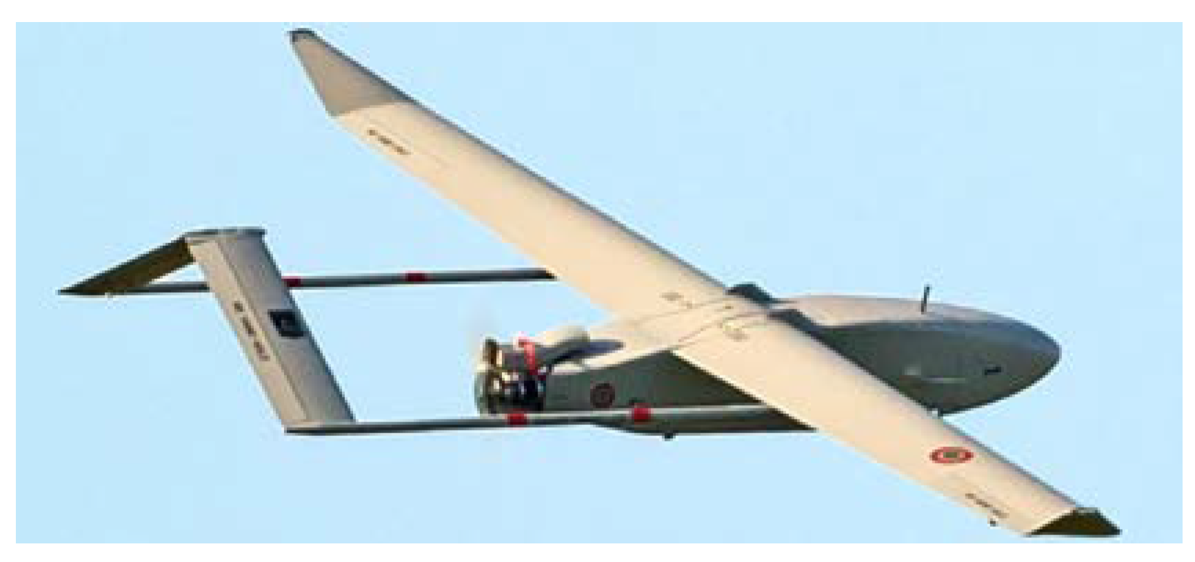
2.1. UAV Basic Characteristics

As a reference application, the lightweight fixed-wing long-endurance UAV Rapier X-25, manufactured by Sky Eye Systems (Foligno, Italy) [12] was considered, Figure 1 and Table 1.

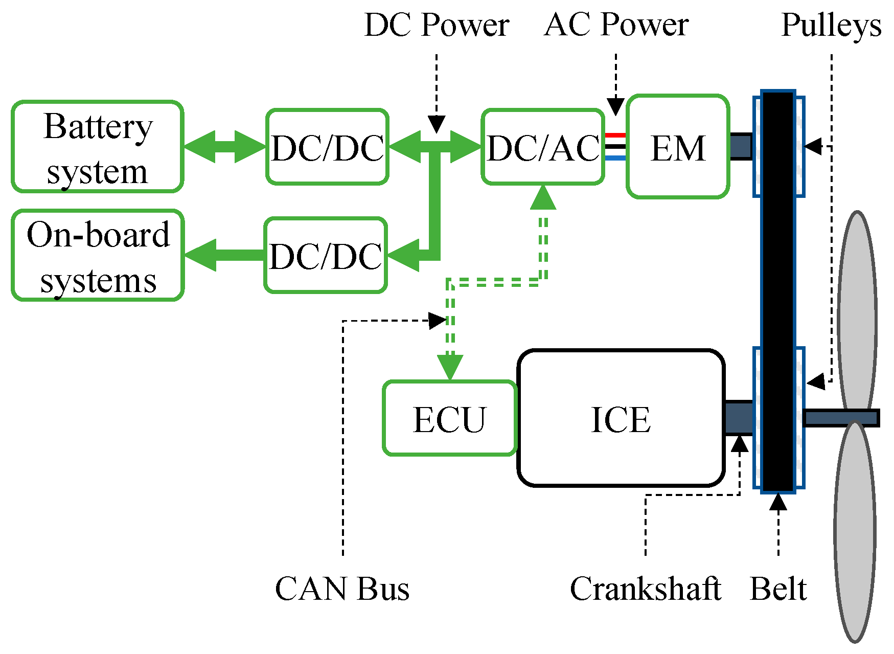
2.2. Propulsion System Description

The propulsion system of the reference UAV, schematically reported in Figure 2, is essentially composed of the following:
  • A two-stroke SI ICE with single cylinder and electronic fuel, equipped with a dedicated Engine Control Unit (ECU) for the spark advance control, the speed control, and the basic monitoring functions [18] and Table 2;
  • A twin-blade fixed-pitch propeller [19];
  • A three-phase brushless DC Electric Machine (EM), used as ICE starter and generator for conventional operation [20];
  • A belt-pulley mechanical transmission, connecting in parallel arrangement the ICE and the EM;
  • A Li-Po battery pack for emergency operations [21];
  • On-board systems, including flight controls and payload.

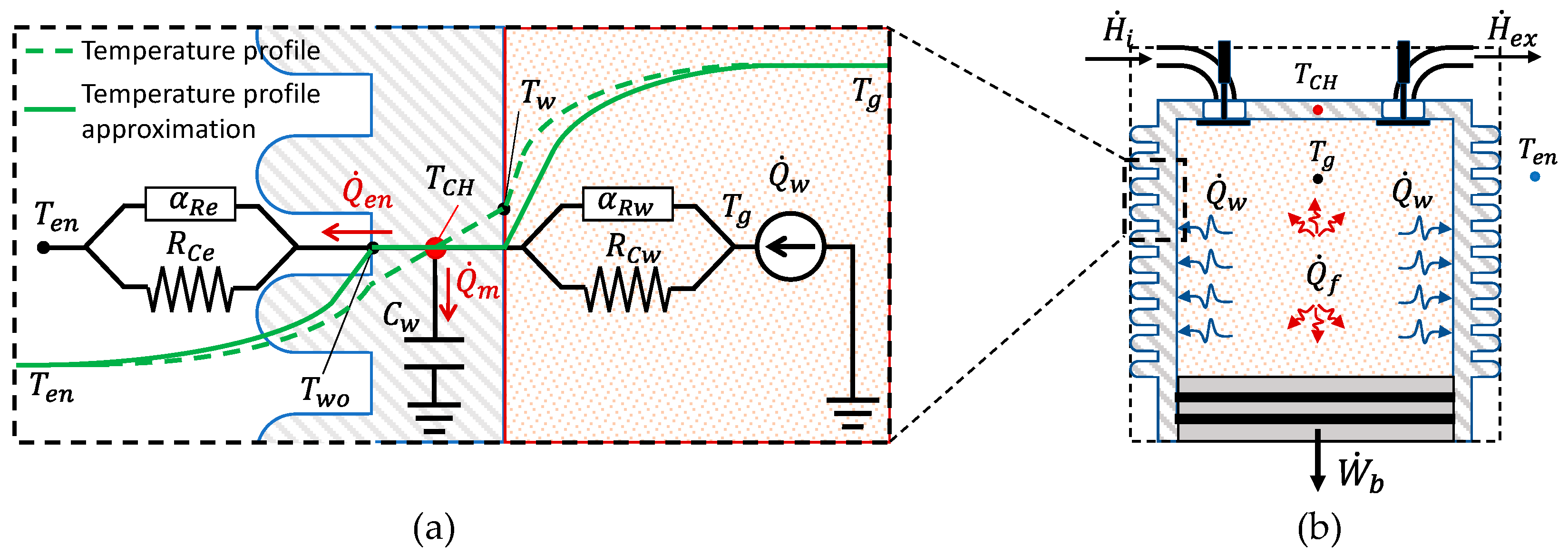
2.3. 0D-SZ Model of the CHT Dynamics

The temperature modelling of the ICE is here addressed using a 0D-SZ approach, which, disregarding the spatial gradients of the temperature field, assumes uniform mixture temperature and composition in the entire combustion chamber.
The CHT dynamics are described by employing an electrical analogy as shown in Figure 3a, where the heat transferred through the ICE cylinder wall is in-part stored in the cylinder walls ( Q m ) and in-part dissipated through convection and radiation towards the environment ( Q e n ). Assuming a thin and highly conductive cylinder wall, the heat balance can be written as follows [22,23,24,25]:
Q ˙ w = Q ˙ m + Q ˙ e n = C w T ˙ C H + 1 R C e T C H T e n + 1 α R e ( T C H 4 T e n 4 )
where C w is the wall thermal capacity, R C e and α R e are the convection and radiation thermal resistances, while T C H and T e ate the cylinder head and environmental temperature, respectively. By rearranging Equation (1), the CHT dynamics can be more explicitly defined by the following:
C w T ˙ C H = Q ˙ w 1 R C e T C H T e n 1 α R e T C H 4 T e n 4 ,
In this work, T C H T and T e n are available measurements, while C w , R C e , α R e , and Q ˙ w are quantities to be identified.
To identify how the term Q ˙ w is correlated to measurable inputs and states of the propulsion system, the energy and mass conservation principles can be applied to the in-cylinder thermodynamic process [7,26,27], Figure 3b:
U ˙ = Q ˙ f Q ˙ w W ˙ b + H ˙ i H ˙ e x H ˙ i = h f m ˙ f + h a m ˙ a H ˙ e x = h e x m ˙ e x m ˙ g = m ˙ a + m ˙ f m ˙ e x ,
where U is the internal energy of the working medium; Q f and Q w are the chemical energy released by the fuel and the heat transfer between the working medium and the cylinder walls, respectively; W b is the work carried out by the in-cylinder pressure; h f , h a , and h e x are the enthalpy related to fuel, intake, and exhaust gas, respectively; m g , m f , m a , and m e x are the total mass, the mass of fuel, intake, and exhaust gasses, respectively.
It is assumed here that the fluid within the control volume is in steady conditions, which implies that the rates of internal energy ( U ˙ ) and total mass ( m ˙ g ) are zero, i.e.:
U ˙ = m g c v T ˙ g = 0 m ˙ a + m ˙ f m ˙ e x = 0 ,
where c v is the specific heat of the working medium.
The released chemical power ( Q ˙ f ) can be expressed as function of the intake air mass rate through the Air–Fuel-Ratio (AFR) coefficient:
Q ˙ f = H L H V m ˙ f = H L H V m ˙ a A F R ,
in which H L H V is the fuel’s lower heating value, and AFR is assumed to be stoichiometric (i.e., ideal mixture that burns all the fuel with no excess air).
The developed power ( W ˙ b ) by the in-cylinder pressure ( p ) is then given by the product of crankshaft angular speed ( ω ) and resistant torque ( M b ), in turn depending on intake mass flow and angular speed [28,29]:
W ˙ b = p V ˙ = ω M b m ˙ a , ω ,
where V is the work-medium volume. The net enthalpy flow is thus expressed as follows:
H ˙ i H ˙ e x = m ˙ a h e x 1 + 1 A F R h f 1 A F R h a .
Assuming that the air, the fuel, and the exhaust gasses follow the ideal gas behaviour, the specific enthalpies are function of the temperature [30]:
h x = T 0 T x c p , x d T ,
in which x = a , f , e x , T 0 is a reference temperature; T x is the temperature at which the enthalpy of the x -th medium is computed, while c p , x is the specific heat of the x -th medium. Typical values of the specific heat capacity are 1, 2.5, and 1.5 kJ/kg°K for air, fuel, and exhaust gasses, respectively; furthermore, considering that the exhaust temperature is much higher than the one of the air or of the fuel temperature and that the stoichiometric value of AFR in SI engines is about 15 [31,32], then (7) can be reformulated as follows:
H ˙ i H ˙ e x = m ˙ a h e x 1 + 1 A F R h f h e x A F R h a h e x m ˙ a h e x T e x ,
where the exhaust temperature is related to the angular speed and the volumetric efficiency, which is a function of the angular speed and the throttle position [32].
The heat transferred through the ICE cylinder wall can be finally obtained from Equation (1) using Equations (2)–(7):
Q ˙ w = H L H V m ˙ a A F R ω M b m ˙ a , ω + m ˙ a h e x T e x ,
Since the intake mass flow rate ( m ˙ a ) depends on the throttle position ( δ t ), altitude ( z h ) [33], and angular speed ( ω ) [34]. It is convenient for the analysis to express the balance with respect to the heat exchanged with the cylinder walls at sea level ( Q ˙ w S L ), using a scaling function depending on altitude ( g z h ):
Q ˙ w δ t , z h , ω = g z h · Q ˙ w S L ( δ t , ω ) ,
The scaling function g z h here is assumed to have the same structure as the one used for obtaining the ICE-indicated power at a generic altitude once known its value at sea level involving the ratios of atmospheric pressure ( p e ) and temperature ( T e ) at altitude z h [35,36]:
g z h = p e ( z h ) p e S L a ¯ T e S L T e ( z h ) b ¯ .
where p e is the atmospheric pressure, and a ¯ and b ¯ are ICE characteristic constants.
Finally, to account for the heat flow propagation lag in the cylinder, the heat power transferred to the walls is obtained by a first-order Padé approximation with time delay τ w :
Q ¨ w S L + 2 τ w Q ˙ w S L = Q ¨ w S L 0 + 2 τ w Q ˙ w S L 0 .
where Q ˙ w S L 0 is the heat power transferred at sea level with no time delay.

2.4. Particle-Swarm Optimization for Model Identification in Normal Conditions

The parameter identification problem consists of estimating the element ϵ ^ that minimizes a cost function J , i.e.:
ϵ ^ = a r g min ϵ E   J ϵ , ϵ ^ ,
where the model parameter to be estimated ϵ belongs to the a priori knowledge set E , and the cost function is defined as follows:
J ϵ , ϵ ^ = r m s T C H ϵ , t T ^ C H ϵ ^ , t ,  
The vector of the parameters to be identified is as follows:
ϵ = C w , R C e , α R e , Q ˙ w S L 0 1 × n · m , a ¯ , b ¯ , τ w T ,
where n   a n d   m are the numbers of breakpoints on signals δ t   a n d   ω for defining Q ˙ w S L 0 .
The optimization problem is solved here via the particle-swarm optimization (PSO) technique [37,38]. The PSO is a heuristic algorithm inspired by the flock behaviour observed in nature, such as schools of fishes or swarms of birds. Each bird of a swarm, while searching randomly for food, can share its own discovery with the other components of the flock, helping them to improve the search. Mathematically, the update in the searching space ( E ) of each vector ( k ) of the swarm ϵ k i + 1 at ( i + 1 ) -th time iteration depends on its current value ϵ k i , on the best current performance p k , and on the best performance on entire set η , (17):
ϵ k i + 1 = ϵ k i + v k i + 1 v k i + 1 = w   v k i + c 1 r 1 p k x k i + c 2 r 2 ( η x k i ) ,
where v k i is the particle velocity, w is an inertia factor, r 1 and r 2 are random vectors within the range [0, 1], while c 1 and c 2 are the so-called cognitive and social coefficients, respectively.

2.5. CHT Modelling in Degraded Conditions

To simulate degradations of the thermal flows, Equation (2) is generalized in the model, by introducing two nondimensional factors, γ Q and γ D ( γ Q , γ D     1 ), so that the model can deviate from normal behaviour in terms of generated and dissipative heat contributions respectively, Equation (18):
C w T ˇ ˙ C H = γ Q Q ˙ w 1 γ D T ˇ C H T e n R C e + T ˇ C H 4 T e n 4 α R e ,
Degradation affecting the produced heat power ( γ D ) can be related to thermal efficiency reduction caused by factors such as improper air–fuel mixture or wrong ignition timing. A rich mixture leads to incomplete combustion and excessive heat, while a lean mixture causes faster combustion and higher engine temperatures [39]. Similarly, advanced ignition timing results in premature combustion, raising peak pressures and temperatures, whereas retarded timing leads to incomplete combustion and higher exhaust gas temperatures [40]. On the other head, efficient heat dissipation in a spark-ignition engine relies on proper airflow channels, free air passages through coolant fins, clean surfaces. Obstructed paths reduce the cooling-air reaching the engine, spoiling convective cooling. Prolonged exposure to high temperatures can cause thermal fatigue, reducing the material ability to emit radiant heat effectively.

2.6. Condition-Based Extended Kalman Filter for CHT Estimation in Degraded Conditions
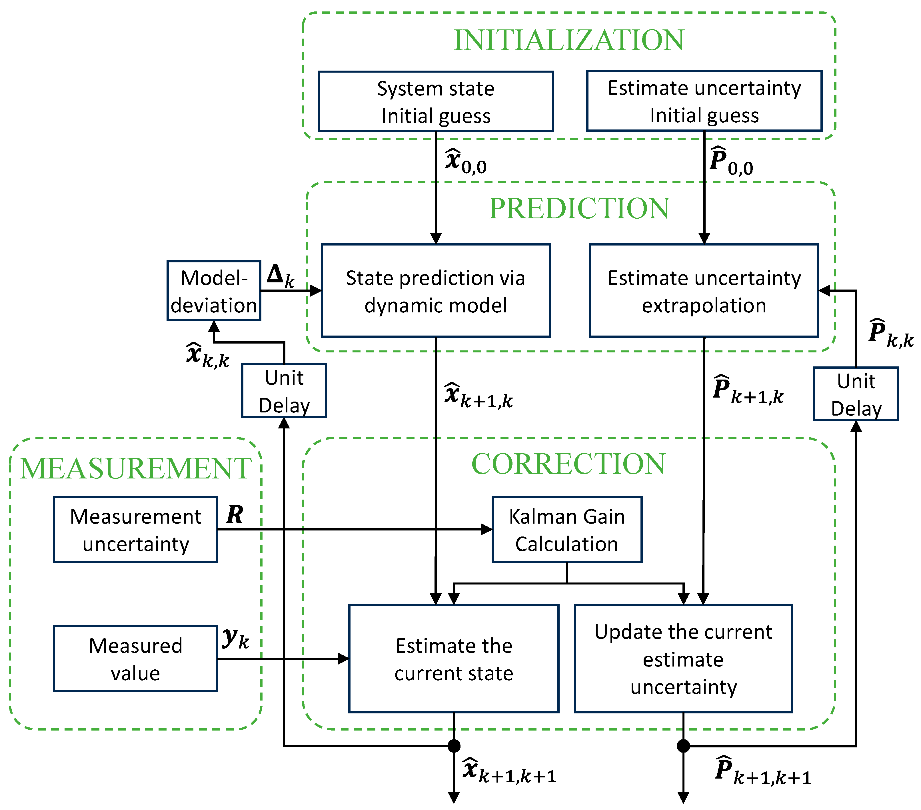
The Kalman Filter (KF) is an optimal state estimator for linear dynamic systems perturbed by white noise, using measurements that are linear functions of the states but corrupted by white noise. Nevertheless, it can be extended to the state estimation of nonlinear dynamic systems by linearizing them via the first or second-order terms of the Taylor series expansion at each time step, resulting in the Extended Kalman Filter (EKF) [13]. The standard KF operates under the assumption that process and measurement noise signals are normally distributed around zero value. Nevertheless, if the system behaviour deviates from a reference modelling with non-zero mean perturbations, the standard KF does not perform optimally. This can occur when the system is affected by degradations. In the proposed condition-based EKF (CBEKF) approach (where “condition” refers to the degradation state), the state of the degraded system is obtained by adding to the standard formulation a model-deviation term, estimating the variation of the state derivative due to degradation. Beyond that enhancing the state estimation, this term can be used for the condition-monitoring of the system (here, the engine).
In a discrete-time formulation, the state vector estimation at step k + 1 ( x k + 1 ) and the measurements vector at step k ( y k ) are as follows:
x k + 1 = f x k ,   u k + w k y k = h ( x k ,   u k ) + v k ,
where f and h are nonlinear functional vectors of the state ( x k ) and the input ( u k ) at step k , while w k ~ N ( 0 ,   Q ) and v k ~ N ( 0 ,   R ) are the system and the measurement zero-mean noise characterized by covariance matrices Q and R , respectively.
Once the system model is defined, with reference to Figure 4, the basic computational for the CBEKF estimator are as follows:
  • Initialization: set a state estimate ( x ^ 0,0 ) and a state estimation error covariance matrix ( P ^ 0,0 ) at time step 0.
  • Prediction: predict the state ( x ^ k + 1 , k ) and the state error covariance matrix ( P ^ k + 1 , k ) ahead (a priori) at time step k + 1 conditioned by measurements at time step k :
    x ^ k + 1 , k = f x ^ k , k ,   u k + w k + Δ k Δ k = f x k ,   u k f x ^ k ,   u k P ^ k + 1 , k = F k P ^ k , k F k T + Q ,
    where Δ k is the model-deviation term that, estimating the state derivative variation due to degradation, corrects the standard EKF formulation, and F k is the Jacobian matrix of the dynamic model with respect to the state evaluated at time step k :
    F k = f x ^ ,   u x ^ x ^ = x ^ k , k ,
  • Correction: compute the Kalman gain ( K k + 1 ), update the state estimate ( x ^ k + 1 , k + 1 ) with the measurement y k (a posteriori), and update the state error covariance matrix P ^ k + 1 , k + 1 , as in Equation (22) [13]:
    K k + 1 = P ^ k + 1 , k H k T H k P ^ k + 1 , k H k T + R 1 x ^ k + 1 , k + 1 = x ^ k + 1 , k + K k + 1 ( y k y ^ k ) P ^ k + 1 , k + 1 = ( I K k + 1 H k ) P ^ k + 1 , k
    where I is the identity matrix, and H k is the Jacobian matrix of the measurement model with respect to the state variables evaluated at time step k :
    H k = h x ^ ,   u x ^ x ^ = x ^ k , k

2.7. CHT Estimation in Degraded Conditions via CBEKF

In the reference case study, the CBEKF is employed to estimate a single state ( x k + 1 ), namely the CHT, so that the state and measurement equation model in Equation (19) can be specialized as follows:
x k + 1 = f x k ,   u k + w k y k = h ( x k ) + v k
where the input vector is u k = δ t , ω , z h , T e , V C A S T . The filter equations are considerably simplified because the involved matrices reduce to scalars, while Equations (20) and (22) reduce into Equations (25) and (26):
x ^ k + 1 , k = f x ^ k , k ,   u k + w k + Δ k Δ k = f x k ,   u k f x ^ k ,   u k P ^ k + 1 , k = F k 2 P ^ k , k + Q
K k + 1 = P ^ k + 1 , k H k / H k 2 P ^ k + 1 , k + R x ^ k + 1 , k + 1 = x ^ k + 1 , k + K k + 1 ( y k y ^ k ) P ^ k + 1 , k + 1 = ( 1 K k + 1 H k ) P ^ k + 1 , k
Given the low-resolution quantization (1 °C) of the CHT sensor, modelled by a round function, and the EKF’s requirement for a differentiable sensor model, a sigmoid-based function is employed to approximate the nonlinear round function. The sigmoid ensures a smooth approximation with a finite derivative, satisfying the EKF’s requirements. The resulting sigmoid-based measurement model is presented in Equations (27) and (28):
h x ^ = x ^ + σ ( a   x ^ x ^ b )
σ ( z ) = 1 / ( 1 + e z )
where x ^ is the floor function applied to x ^ , σ is the sigmoid function, a and b are parameters controlling the steepness of the transition and the sensor quantization interval.
h x ^ x ^ = a   σ a   x ^ x ^ b 1 σ a   x ^ x ^ b
Figure 5 reports an example of the measurement sensitivity model and its derivative as a function of the state variable once given a = 100 and b = 0.5. The figure highlights how the sigmoid function closely approximates the round function while ensuring the necessary derivative properties for EKF implementation.
When the measurement does not change level, the probability distribution within the current quantized interval can be uniformly or normally distributed with a certain standard deviation, depending on the instrument, and there is no additional information suggesting that one point within the interval is more likely than another. However, when a measurement changes level, it occurs that the midpoint of the quantization interval is statistically more likely to be closer to the true state. This additional consideration can help the Kalman filter converge faster to the true state. To enhance this process, a CBEKF with AUtomatic reset (CBEKF-AU) can be employed. When a measurement update is detected, the filter is re-initialized to the midpoint of the quantization interval, providing a more balanced starting point and a faster convergence. However, if the sensor resolution is poor, the initial estimate based on a single measurement may be far from the true state. The Kalman filter will then take more iterations to correct the initial state estimate as it incorporates more measurements and the process mode.

3. Results and Discussion

This section summarizes the results related to the model validation in normal condition as well as to the CHT estimation in degraded conditions, by applying the EKF, the CBEKF, and the CBEKF-AU illustrated in the previous section.
The thermodynamic model and the CHT estimation algorithm have been entirely developed in the MATLAB/Simulink 2023b environment, and their numerical solution has been obtained via the fourth-order Runge–Kutta method, with a 0.02 s integration step.

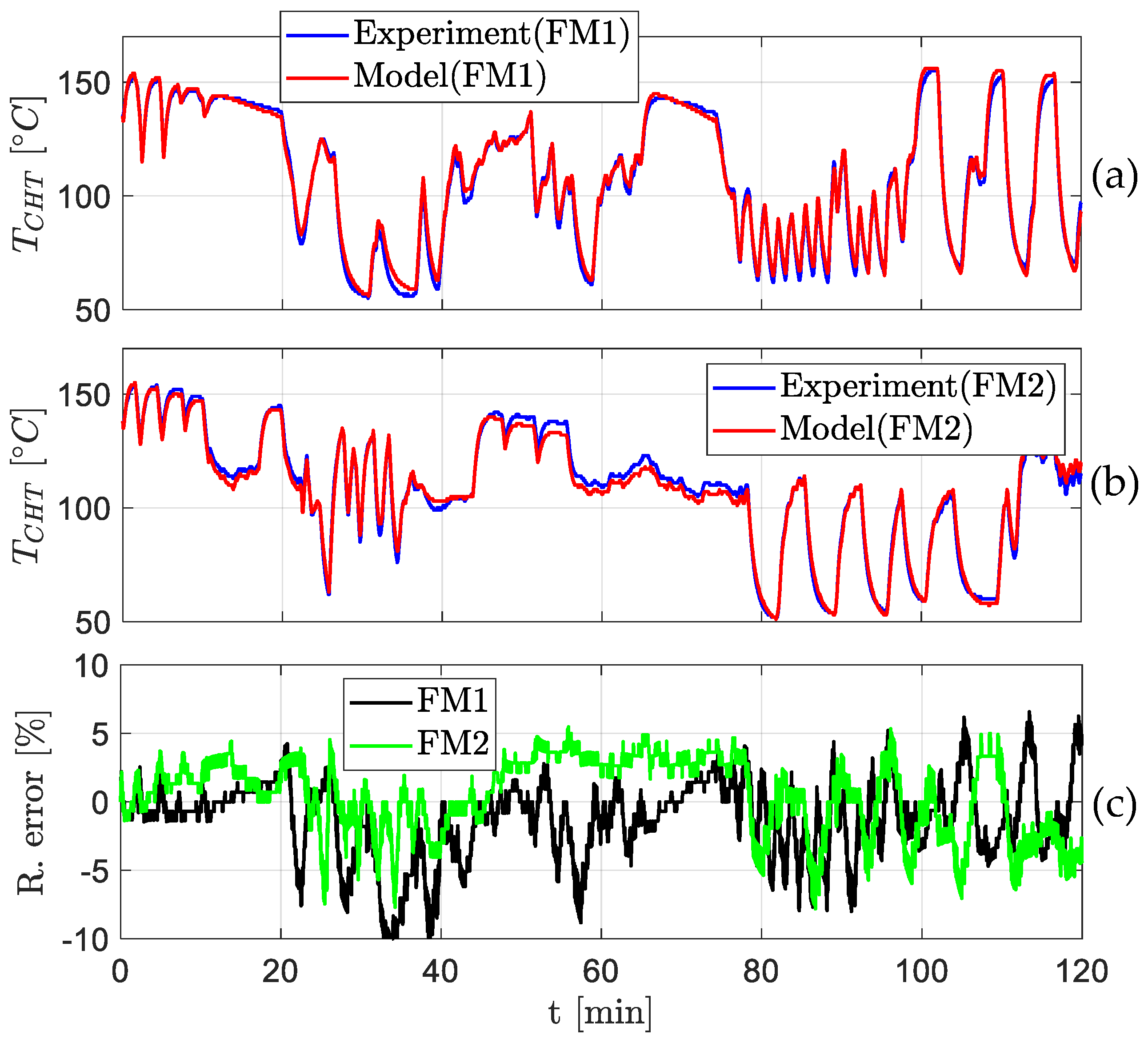
3.1. Model Validation in Nominal Conditions with Experimental Flight Data

The parameters of the nominal model have been identified and validated using experimental data coming from two flight missions (FM1 and FM2, Appendix A). Specifically, the first dataset has been used for the model parameters identification via PSO algorithm, while the second dataset has been used to validate the model accuracy.
Figure 6 compares the simulated and experimental time histories values of the CHT: in particular, Figure 6a reports the results related to the dataset used for the parameters identification (FM1), while Figure 6b shows the validation results (FM2). Figure 6c points out that the mean and peak errors are lower than 2% and 10%.

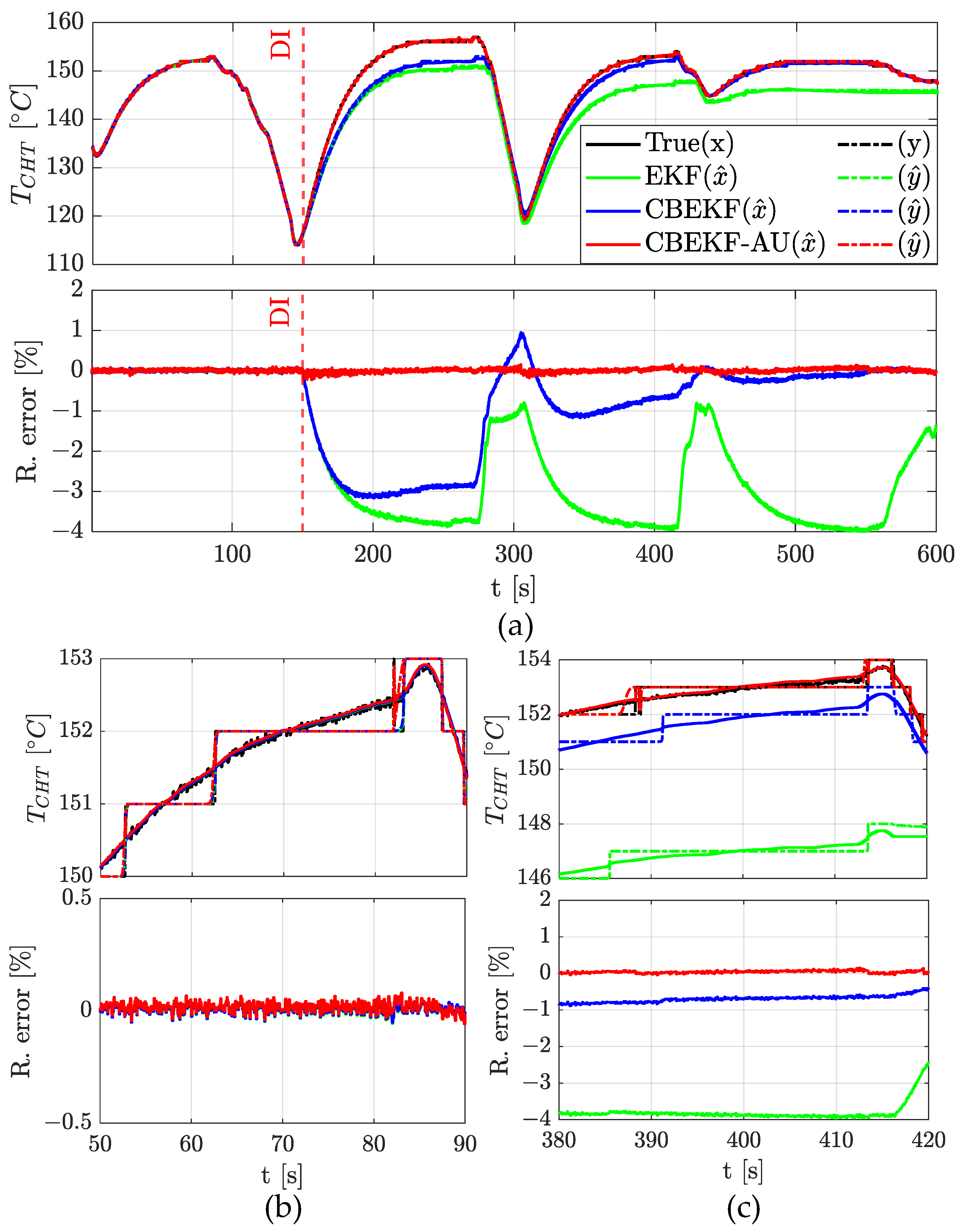
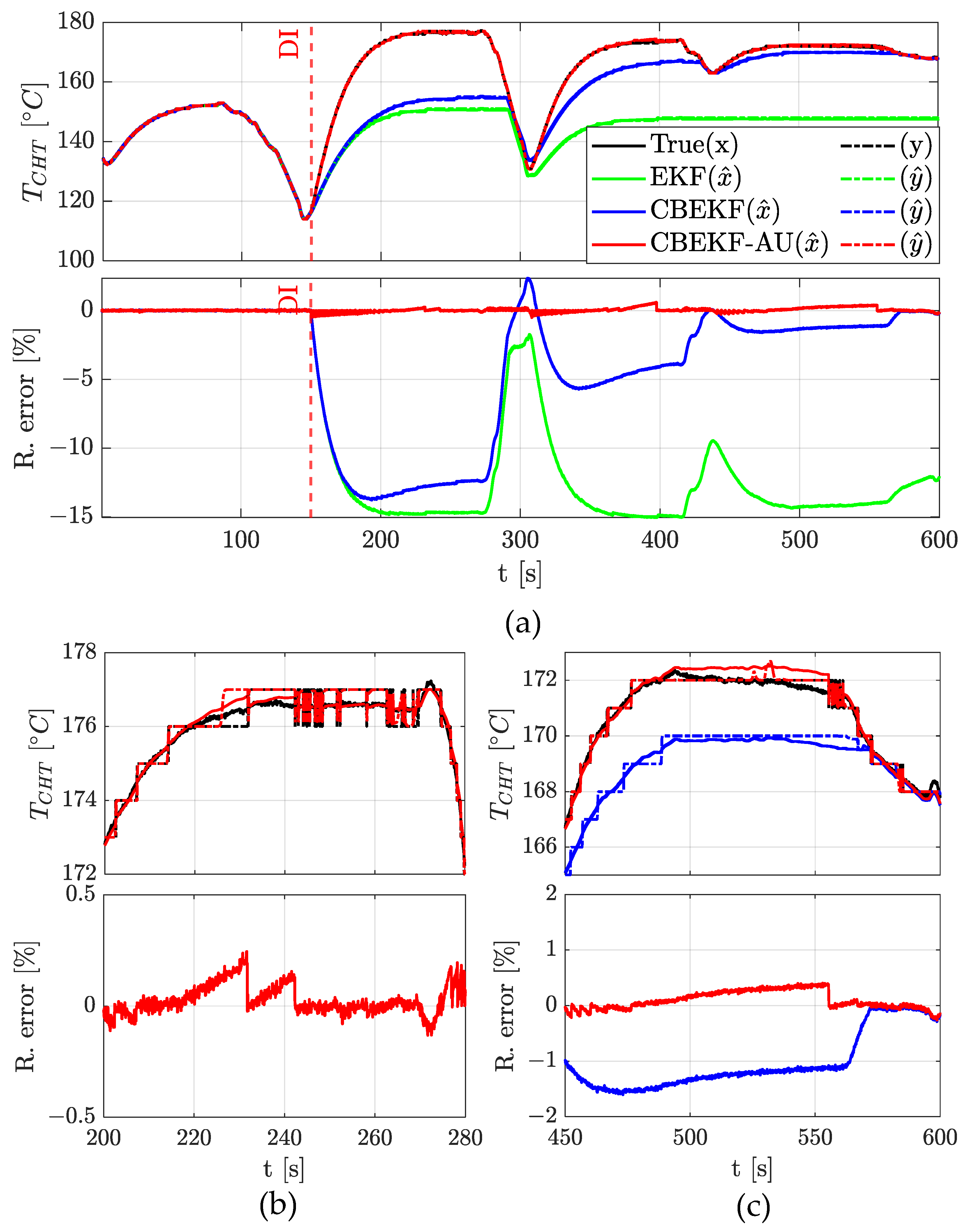
3.2. CHT Estimation via EKF Strategies and Thermal Flow Monitoring

Figure 7 shows a simulation of the CHT and its estimation with a degradation injection (DI) of γ Q = 1.1 at time t = 150 s. The figure compares the proposed approach with a conventional EKF ( Δ k = 0 in Equation (19)). When the ICE operates in nominal conditions, all strategies yield the same results, Figure 7b. On the other hand, when the degradation is injected, the conventional EKF does not converge to the measured CHT (exhibiting a prediction error from 1% to 4%), while both CBEKF-based strategies converge to it, even if with very different time scales. In particular, the converging time is extremely small if the CBEKF-AU is applied, while it reaches about 300 s by using a CBEKF without initial condition reset, Figure 7c.
To further evaluate the capability of the CBEKF-AU in estimating CHT in degraded conditions, another test, similar to the previous one, was carried out, with a high degradation factor ( γ Q = 1.5 ), causing the temperature to significantly increase (+20 °C) with respect to nominal conditions. The results, shown in Figure 8, highlight that the relative error increases, though remaining lower than 1%, which is lower than the quantization step.
A summary of the error distribution for the CHT estimation using the CBEKF-AU strategy with respect to increasing levels of degradation γ Q is proposed in Figure 9 in terms of box plots. The distribution, which is verified to be well approximated by a normal distribution, shows a linear increase in its standard deviation if degradation level increases. Additionally, there is a drift of the mean error for degradation levels greater than γ Q = 1.3 . Furthermore, for values greater than 1.3, both the interquartile range and the whiskers grow linearly, suggesting a decrease in consistency and an increase in the spread of the data. This indicates greater variability, particularly in the tails of the distribution. Nevertheless, this is expected, as values higher than 20–30% no longer represent degradation of the system but rather a fault or an entirely different system.
Another relevant outcome of the proposed work is the detection of thermal degradation. Indeed, the CBEKF approach is based on the estimation of model-deviation term Δ k , which can also be leveraged as symptom of thermal flow degradation. Figure 10 reports the model-deviation term ( Δ k ) for two values of the degradation factor γ Q . The degradation symptom responds instantaneously to the degradation injection, and it is characterized by a non-null mean value. It is worth noting that, despite some fluctuations, within the first 50 s after the degradation injection, the time derivative of the model-deviation term is roughly linear with respect to the degradation level. The value of the model-deviation term derivative after 10 s for different combined values of degradation factors γ Q and γ D are presented in Figure 11, pointing out that the derivative increases linearly with the severity of the degradation.

4. Conclusions and Future Developments

A novel 0D-SZ model of the CHT dynamics in SI ICEs for UAVs is developed from physical first principles and validated for nominal thermal flow conditions with respect to the flight data of a long-endurance fixed-wing UAV (mean and peak errors are lower than 2% and 10%, respectively). The proposed dynamic model accounts for the heat flow propagation lag in the cylinder and incorporates dependencies on throttle position, angular speed, UAV airspeed, and altitude, quantities that are all available in real time to the engine-health-monitoring system. The model is then employed to create a monitoring algorithm that incorporates a condition-based EKF with initial condition reset. The estimation performance of the so-called CBEKF-AU strategy is compared with a conventional EKF and with a CBEKF without initial reset, demonstrating its effectiveness. At this stage, the proposed approach serves as an effective tool for detecting degradation. Future work will focus on isolating the degradation to determine which specific engine component is affected, though this will require increasing the complexity of the dynamic model. Simulations show that while the mean error remains close to zero, the interquartile range of the estimation error grows linearly with the degradation amplitude introduced into the system. Nevertheless, it remains below 1% for up to 50% degradation compared to the nominal condition. This approach enables near-instantaneous detection of thermal degradation, facilitating timely predictive maintenance and mitigating the risk of ICE thermal fatigue, performance degradation, and failure.

Author Contributions

Conceptualization, A.S.; methodology, A.S.; software, A.S.; validation, A.S. and G.D.R.; formal analysis, A.S.; investigation, A.S.; resources, G.M.; data curation, A.S.; writing—original draft preparation, A.S.; writing—review and editing, A.S. and G.D.R.; visualization, A.S. and G.D.R.; supervision, G.D.R.; project administration, G.D.R.; funding acquisition, G.D.R. and G.M. All authors have read and agreed to the published version of the manuscript.

Funding

This research received no external funding.

Data Availability Statement

The original contributions presented in the study are included in the article, further inquiries can be directed to the corresponding author.

Conflicts of Interest

The authors declare no conflicts of interest.

Appendix A

This section reports the following:
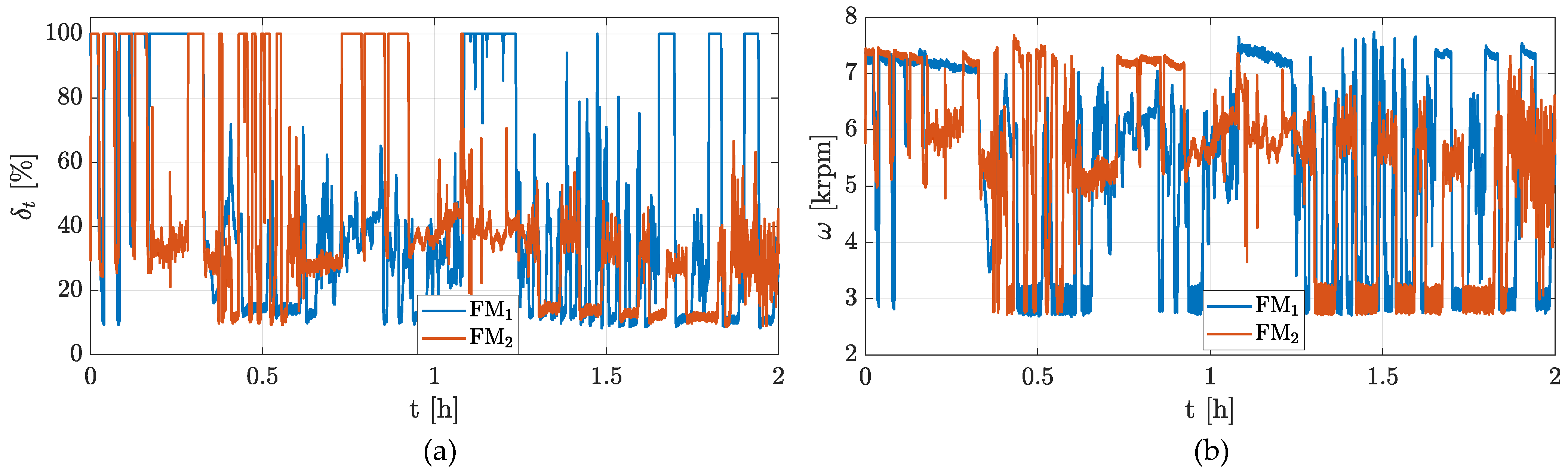
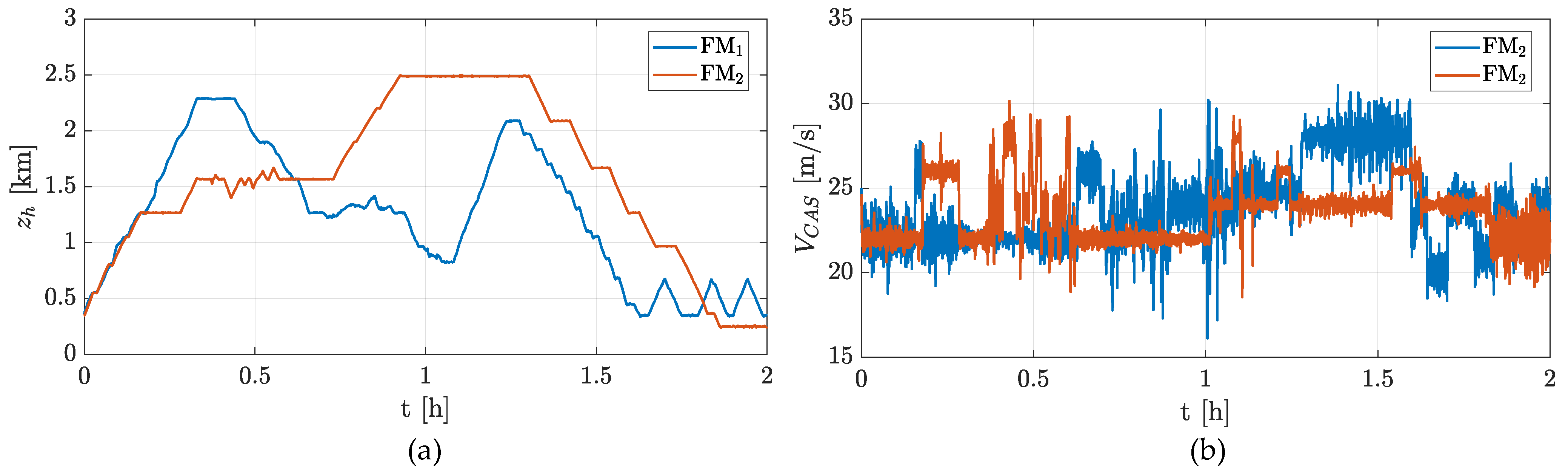
  • The experimental data used in this work (The experimental data, which are proprietary to the company, can only be shared in graphical form. Readers interested in obtaining the numerical data file should contact the company Sky Eye Systems s.r.l. (Foligno, Italy) directly) are provided as time histories. The Rapier X-25 system integrates a ground control station that, via the datalink, allows both mission execution and real-time monitoring of key system data. These data are provided below: Figure A1 reports the throttle position ( δ t ) and crankshaft angular speed ( ω ); Figure A2 reports the altitude ( z h ) and calibrated air speed of the UAV ( V C A S ); Figure A3 reports the CHT ( T C H ) and the outside air temperature ( T e ).
  • The model parameters and function, Table A1 and Figure A4, identified by the PSO technique.
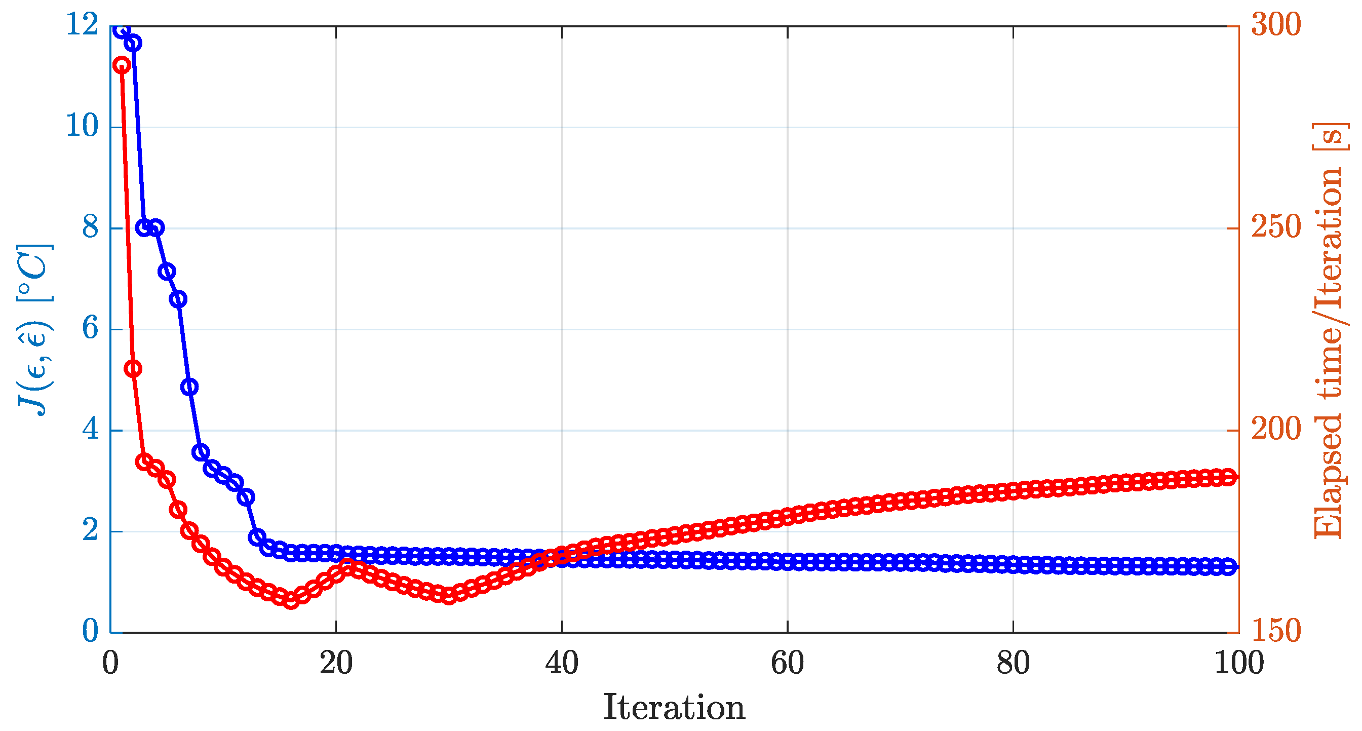
  • The PSO cost function and elapsed time over 100 iteration, Figure A5.
Figure A1. Flight measurements during FM1 and FM2: (a) throttle position; (b) ICE angular speed.
Drones 08 00531 g0a1
Figure A2. Flight measurements during FM1 and FM2: (a) altitude; (b) calibrated airspeed.
Drones 08 00531 g0a2
Figure A3. Flight measurements during FM1 and FM2: (a) CHT; (b) outside air temperature.
Drones 08 00531 g0a3
Table A1. Model parameters identified by PSO.
ParameterValueUnit
C w 570J/°C
R C e n 0.15W/°C
α R e n 8.1 × 10⁵W/°C4
τ w 6s
a ¯ 1.55-
b ¯ 2-
Figure A4. Heat-generated power at sea level as a function of throttle position and angular speed.
Drones 08 00531 g0a4
Figure A5. PSO cost function (blue line) and elapsed time per iteration (red line).
Drones 08 00531 g0a5

References

  1. Suti, A.; Di Rito, G.; Galatolo, R. Climbing Performance Enhancement of Small Fixed-Wing UAVs via Hybrid Electric Propulsion. In Proceedings of the 2021 IEEE Workshop on Electrical Machines Design, Control and Diagnosis (WEMDCD), Modena, Italy, 8–9 April 2021; IEEE: Piscataway, NJ, USA, 2021; pp. 305–310. [Google Scholar]
  2. Silva, F.S. Fatigue on Engine Pistons—A Compendium of Case Studies. Eng. Fail. Anal. 2006, 13, 480–492. [Google Scholar] [CrossRef]
  3. Thomaz, F.; Teixeira Malaquias, A.C.; Resende de Paula, G.A.; Baêta, J.G.C. Thermal Management of an Internal Combustion Engine Focused on Vehicle Performance Maximization: A Numerical Assessment. Proc. Inst. Mech. Eng. Part D J. Automob. Eng. 2021, 235, 2296–2310. [Google Scholar] [CrossRef]
  4. Fonseca, L.; Olmeda, P.; Novella, R.; Valle, R.M. Internal Combustion Engine Heat Transfer and Wall Temperature Modeling: An Overview. Arch. Comput. Methods Eng. 2020, 27, 1661–1679. [Google Scholar] [CrossRef]
  5. Broatch, A.; Olmeda, P.; Margot, X.; Escalona, J. New Approach to Study the Heat Transfer in Internal Combustion Engines by 3D Modelling. Int. J. Therm. Sci. 2019, 138, 405–415. [Google Scholar] [CrossRef]
  6. Marinoni, A.; Tamborski, M.; Cerri, T.; Montenegro, G.; D’Errico, G.; Onorati, A.; Piatti, E.; Pisoni, E.E. 0D/1D Thermo-Fluid Dynamic Modeling Tools for the Simulation of Driving Cycles and the Optimization of IC Engine Performances and Emissions. Appl. Sci. 2021, 11, 8125. [Google Scholar] [CrossRef]
  7. Mauro, S.; Şener, R.; Gül, M.Z.; Lanzafame, R.; Messina, M.; Brusca, S. Internal Combustion Engine Heat Release Calculation Using Single-Zone and CFD 3D Numerical Models. Int. J. Energy Environ. Eng. 2018, 9, 215–226. [Google Scholar] [CrossRef]
  8. Sjeric, M.; Kozarac, D.; Bogensperger, M. Implementation of a Single Zone K-ε Turbulence Model in a Multi Zone Combustion Model. In Proceedings of the SAE 2012 World Congress & Exhibition, Detroit, MI, USA, 24–26 April 2012. [Google Scholar]
  9. Giglio, V.; di Gaeta, A. Novel Regression Models for Wiebe Parameters Aimed at 0D Combustion Simulation in Spark Ignition Engines. Energy 2020, 210, 118442. [Google Scholar] [CrossRef]
  10. Boiarciuc, A.; Floch, A. Evaluation of a 0D Phenomenological SI Combustion Model. In Proceedings of the SAE International Powertrains, Fuels and Lubricants Meeting, Kyoto, Japan, 30 August–2 September 2011. [Google Scholar]
  11. Payri, F.; Olmeda, P.; Martín, J.; García, A. A Complete 0D Thermodynamic Predictive Model for Direct Injection Diesel Engines. Appl. Energy 2011, 88, 4632–4641. [Google Scholar] [CrossRef]
  12. Liu, Z.; Liu, J. Investigation of the Effect of Simulated Atmospheric Conditions at Different Altitudes on the Combustion Process in a Heavy-Duty Diesel Engine Based on Zero-Dimensional Modeling. J. Eng. Gas. Turbine Power 2022, 144, 061013. [Google Scholar] [CrossRef]
  13. Grewal, M.S.; Andrews, A.P. Kalman Filtering; Wiley: Hoboken, NJ, USA, 2008; ISBN 9780470173664. [Google Scholar]
  14. Lu, F.; Lv, Y.; Huang, J.; Qiu, X. A Model-Based Approach for Gas Turbine Engine Performance Optimal Estimation. Asian J. Control 2013, 15, 1794–1808. [Google Scholar] [CrossRef]
  15. Simon, D. A Comparison of Filtering Approaches for Aircraft Engine Health Estimation. Aerosp. Sci. Technol. 2008, 12, 276–284. [Google Scholar] [CrossRef]
  16. Lu, F.; Ju, H.; Huang, J. An Improved Extended Kalman Filter with Inequality Constraints for Gas Turbine Engine Health Monitoring. Aerosp. Sci. Technol. 2016, 58, 36–47. [Google Scholar] [CrossRef]
  17. Liu, X.; Zhu, J.; Luo, C.; Xiong, L.; Pan, Q. Aero-Engine Health Degradation Estimation Based on an Underdetermined Extended Kalman Filter and Convergence Proof. ISA Trans. 2022, 125, 528–538. [Google Scholar] [CrossRef] [PubMed]
  18. Currawong Engineering. CORVID-29. Available online: https://www.currawongeng.com/corvid-29/ (accessed on 12 August 2024).
  19. APC—INTERNAL COMBUSTION ENGINES/SPORT/18 × 8. Available online: https://www.apcprop.com/product/18x8/ (accessed on 12 August 2024).
  20. Maxon. View Product, Motor. Available online: https://www.maxongroup.it/maxon/view/product/motor/ecmotor/ec4pole/305015 (accessed on 15 October 2023).
  21. Maxamps Lithium Batteries. LiPo 1850 6S 22.2v Battery Pack. Available online: https://maxamps.com (accessed on 15 October 2023).
  22. Memon, Z.K.; Sundararajan, T.; Lakshminarasimhan, V.; Babu, Y.R.; Harne, V. Parametric Study on Fin Heat Transfer for Air Cooled Motorcycle Engine. In Proceedings of the International Mobility Engineering Congress & Exposition 2005—SAE India Technology for Emerging Markets, Chennai, India, 23 October 2005. [Google Scholar]
  23. Sachar, S.; Parvez, Y.; Khurana, T.; Chaubey, H. Heat Transfer Enhancement of the Air-Cooled Engine Fins through Geometrical and Material Analysis: A Review. Mater. Today Proc. 2023. [Google Scholar] [CrossRef]
  24. Reddy Kummitha, O.; Reddy, B.V.R. Thermal Analysis of Cylinder Block with Fins for Different Materials Using ANSYS. Mater. Today Proc. 2017, 4, 8142–8148. [Google Scholar] [CrossRef]
  25. Suti, A.; Di Rito, G.; Mattei, G. Model-Based Temperature Monitoring of the Internal Combustion Engine of a Lightweight Long-Endurance Fixed-Wing UAV. In Proceedings of the 2024 11th International Workshop on Metrology for AeroSpace (MetroAeroSpace), Lublin, Poland, 3–5 June 2024; IEEE: Piscataway, NJ, USA, 2024; pp. 254–259. [Google Scholar]
  26. Zhang, C.; Chen, F.; Li, L.; Xu, Z.; Liu, L.; Yang, G.; Lian, H.; Tian, Y. A Free-Piston Linear Generator Control Strategy for Improving Output Power. Energies 2018, 11, 135. [Google Scholar] [CrossRef]
  27. Abedin, M.J.; Masjuki, H.H.; Kalam, M.A.; Sanjid, A.; Rahman, S.M.A.; Masum, B.M. Energy Balance of Internal Combustion Engines Using Alternative Fuels. Renew. Sustain. Energy Rev. 2013, 26, 20–33. [Google Scholar] [CrossRef]
  28. Ashok, B.; Denis Ashok, S.; Ramesh Kumar, C. Trends and Future Perspectives of Electronic Throttle Control System in a Spark Ignition Engine. Annu. Rev. Control 2017, 44, 97–115. [Google Scholar] [CrossRef]
  29. Le Solliec, G.; Le Berr, F.; Colin, G.; Corde, G.; Chamaillard, Y. Engine Control of a Downsized Spark Ignited Engine: From Simulation to Vehicle. Oil Gas Sci. Technol.—Rev. L’IFP 2007, 62, 555–572. [Google Scholar] [CrossRef]
  30. Payri, F.; Olmeda, P.; Martín, J.; Carreño, R. Experimental Analysis of the Global Energy Balance in a DI Diesel Engine. Appl. Therm. Eng. 2015, 89, 545–557. [Google Scholar] [CrossRef]
  31. Heywood, J.B. Internal Combustion Engine Fundamentals, 2nd ed.; McGraw-Hill Education: New York, NY, USA, 2018. [Google Scholar]
  32. Kalantzis, N.; Pezouvanis, A.; Ebrahimi, K.M. Internal Combustion Engine Model for Combined Heat and Power (CHP) Systems Design. Energies 2017, 10, 1948. [Google Scholar] [CrossRef]
  33. Hassantabar, A.; Najjaran, A.; Farzaneh-Gord, M. Investigating the Effect of Engine Speed and Flight Altitude on the Performance of Throttle Body Injection (TBI) System of a Two-Stroke Air-Powered Engine. Aerosp. Sci. Technol. 2019, 86, 375–386. [Google Scholar] [CrossRef]
  34. Lee, G.; Myung, C.-L.; Park, S.; Cho, Y. Sensitivity of Hot Film Flow Meter in Four Stroke Gasoline Engine. KSME Int. J. 2004, 18, 286–293. [Google Scholar] [CrossRef]
  35. Lapuerta, M.; Armas, O.; Agudelo, J.R.; Sánchez, C.A. Estudio Del Efecto de La Altitud Sobre El Comportamiento de Motores de Combustión Interna. Parte 1: Funcionamiento. Inf. Tecnol. 2006, 17, 21–30. [Google Scholar] [CrossRef]
  36. Ceballos, J.J.; Melgar, A.; Tinaut, F.V. Influence of Environmental Changes Due to Altitude on Performance, Fuel Consumption and Emissions of a Naturally Aspirated Diesel Engine. Energies 2021, 14, 5346. [Google Scholar] [CrossRef]
  37. Wu, Y.; Gou, J.; Ji, H.; Deng, J. Hierarchical Mission Replanning for Multiple UAV Formations Performing Tasks in Dynamic Situation. Comput. Commun. 2023, 200, 132–148. [Google Scholar] [CrossRef]
  38. Suti, A.; Di Rito, G.; Mattei, G. Heuristic Estimation of Temperature-Dependant Model Parameters of Li-Po Batteries for UAV Applications. In Proceedings of the 2023 IEEE 10th International Workshop on Metrology for AeroSpace (MetroAeroSpace), Milan, Italy, 19–21 June 2023; IEEE: Piscataway, NJ, USA, 2023; pp. 269–274. [Google Scholar]
  39. Speight, J.G. Handbook of Industrial Hydrocarbon Processes, 2nd ed.; Elsevier: Amsterdam, The Netherlands, 2019; ISBN 9780128099230. [Google Scholar]
  40. Koksal, H.; Ceviz, M.A.; Yakut, K.; Kaltakkiran, G.; Özakin, A.N. A Novel Ignition Timing Strategy to Regulate the Energy Balance during the Warm up Phase of an SI Engine. Case Stud. Therm. Eng. 2023, 41, 102602. [Google Scholar] [CrossRef]
Figure 1. UAV Rapier X-25, manufactured by Sky Eye Systems (Foligno, Italy).
Drones 08 00531 g001
Figure 2. Schematic of the reference propulsion system.
Drones 08 00531 g002
Figure 3. Thermal flows in the combustion chamber: (a) reference scheme of heat transfer from the chamber walls to environment; (b) in-cylinder thermodynamic process.
Drones 08 00531 g003
Figure 4. CBEKF block diagram.
Drones 08 00531 g004
Figure 5. Example of a measurement quantization (b = 0.5) with raw and sigmoid-based transition at a = 100 (top) and measurement sigmoid-based derivative with respect to state (bottom).
Drones 08 00531 g005
Figure 6. Experimental and simulated CHT time histories: (a) FM1, (b) FM2, (c) errors.
Drones 08 00531 g006
Figure 7. CHT estimation with degradation injection (DI) at γ Q = 1.1 ,     γ D = 1 : (a) whole time history; (b) detail on nominal conditions regime; (c) detail on degraded conditions regime.
Drones 08 00531 g007
Figure 8. CHT estimation with degradation injection (DI) at γ Q = 1.5 ,     γ D = 1 : (a) whole time history; (b) detail on nominal conditions regime; (c) detail on degraded conditions regime.
Drones 08 00531 g008
Figure 9. Estimation error with CBEKF-AU strategy at increasing values of γ Q ( γ D = 1 ).
Drones 08 00531 g009
Figure 10. Model-deviation term with degradation injection (DI) at γ Q = 1.1   s o l i d   l i n e   a n d   γ Q = 1.5   d o t t e d   l i n e ,   ( γ D = 1 ) .
Drones 08 00531 g010
Figure 11. Model-deviation term derivative 10 s after the degradation injection.
Drones 08 00531 g011
Table 1. UAV Rapier X-25 main characteristics.
CharacteristicValueUnit
Maximum take-off weight25kg
Wingspan3.5m
Total length2.3m
Height 0.7m
Endurance16h
Rate of climb3m/s
Cruise speed23m/s
Maximum operational altitude4000m
Datalink range100km
Table 2. Reference propulsion system main characteristics.
CharacteristicValueUnit
Engine type2-stroke single cylinder-
Total weight3.17kg
Speed operating range [2000, 9000]rpm
Power operating range[0.4, 1.9]kW
Speed at cruise 6000rpm
Power at cruise0.8kW
Fuel consumption at cruise500g/kW-h
Generator continuous power250W
Displacement29cc
Approximated cylinder boar range[36, 38]mm
Approximated cylinder stroke range[26, 28]mm
Time Between Overhaul350h
Coolingair-cooled-
Ability to be started from cold[−20, 50]°C
Disclaimer/Publisher’s Note: The statements, opinions and data contained in all publications are solely those of the individual author(s) and contributor(s) and not of MDPI and/or the editor(s). MDPI and/or the editor(s) disclaim responsibility for any injury to people or property resulting from any ideas, methods, instructions or products referred to in the content.

