Abstract
Recently, developing multi-UAVs to cooperatively pursue a fast-moving target has become a research hotspot in the current world. Although deep reinforcement learning (DRL) has made a lot of achievements in the UAV pursuit game, there are still some problems such as high-dimensional parameter space, the ease of falling into local optimization, the long training time, and the low task success rate. To solve the above-mentioned issues, we propose an improved twin delayed deep deterministic policy gradient algorithm combining the genetic algorithm and maximum mean discrepancy method (GM-TD3) for multi-UAV cooperative pursuit of high-speed targets. Firstly, this paper combines GA-based evolutionary strategies with TD3 to generate action networks. Then, in order to avoid local optimization in the algorithm training process, the maximum mean difference (MMD) method is used to increase the diversity of the policy population in the updating process of the population parameters. Finally, by setting the sensitivity weights of the genetic memory buffer of UAV individuals, the mutation operator is improved to enhance the stability of the algorithm. In addition, this paper designs a hybrid reward function to accelerate the convergence speed of training. Through simulation experiments, we have verified that the training efficiency of the improved algorithm has been greatly improved, which can achieve faster convergence; the successful rate of the task has reached 95%, and further validated UAVs can better cooperate to complete the pursuit game task.
1. Introduction
In modern information warfare, UAVs have received more and more attention from the militaries of various countries [1]. Especially in the Russia–Ukraine war, a large number of practical applications of UAV technology have achieved remarkable results [2], fully demonstrating the key role of UAVs in modern warfare. With the development of unmanned equipment technology, the miniaturization and intelligence of UAVs make it difficult for traditional air defense systems to respond effectively [3]. It can be said that UAVs with low costs, miniaturization, and intelligence, especially AI (artificial intelligence) technology, have shown great war potential in the actual combat environment and have become the “new darling” on the battlefield.
As a typical differential game problem in air combat [4], the UAV pursuit problem can be regarded as a multi-agent dynamic game system due to the conflicting objective functions of both sides [5,6,7]. The choice of the optimal control strategy for UAVs from both sides depends on their respective interests [8,9]. Therefore, advanced intelligent decision-making technology is needed to assist the commanders of UAVs in real-time tactical decision-making and command [10]. These intelligent decision technologies can be implemented using machine learning, artificial intelligence (AI), and autonomous decision algorithms, enabling UAV swarms to autonomously perceive the environment, analyze intelligence, make decisions, and perform tasks. Through AI technologies, commanders can quickly acquire and analyze vast amounts of perception data and receive real-time intelligence and recommendations to support them in making efficient and correct decisions.
Reinforcement learning (RL) is an intelligent self-learning method that does not require expert signals or strict mathematical models. It adopts a trial-and-error mechanism to interact with the environment and constantly tries different behavioral strategies for reinforcement and improvement. RL is self-adaptive to the dynamic and unknown environment; therefore, it is suitable for adaptive optimal control methods with the aim of solving complex nonlinear systems [11]. Based on these characteristics, RL can realize the confrontation or cooperative behavior of multiple agents, and provide reasonable, reliable, and dynamic policy support for multi-agent systems. Therefore, it has good prospects for application in the field of differential games.
To combine the advantages of game theory and the RL algorithm, some scholars introduce RL into the adversarial game modeling process. For example, the multi-agent deep deterministic policy gradient (MADDPG) algorithm proposed by LOWE R et al. adopts the method of decentralized execution of actions and centralized training of strategies [12]; the algorithm has good stability and solves the problem of excessive gradient variance of the strategy. It can enable multi-agents to find cooperative strategies under the environment of both cooperation and competition. The collaborative learning model of the joint action learner is presented in the literature [13], and the effectiveness of this method is proved by experiments. In addition, there are many algorithms from different perspectives, such as the Q algorithm based on correlated equilibrium solutions (CE-Q) [14], the Q algorithm based on Pareto dominant solutions (Pareto-Q) [15], etc. These algorithms provide different research ideas for solving multi-agent reinforcement learning problems.
In the context of intelligent decision-making for UAVs, the literature [16] employs reinforcement learning methods to generate maneuvering strategies aimed at enhancing the survival rate of UAVs in complex aerial combat scenarios. It proposes a unit state sequence (USS) based on deep double Q networks (DDQNs) and deep deterministic policy gradient (DDPG) algorithms, and integrates contextual features from the USS using gated recurrent units (GRUs) to improve the UAV’s capability for state feature recognition and the convergence of the algorithm in intricate aerial combat environments. Reference [17] focuses on the modeling and simulation of disturbances such as wind and obstacles along paths in the context of simulations of the drone swarm environment. The research demonstrates that the presence of these disturbances can significantly alter the deployment and maneuvering decisions of drone swarms within simulated scenarios. An improved method [18] based on the Q-learning algorithm is proposed for the mapping of the paths and obstacle avoidance tasks of unmanned aerial vehicles (UAVs) which is compared with the well-known reinforcement learning algorithm, state–action–reward–state–action (SARSA). During the obstacle avoidance control process, a reinforcement learning approach is similarly employed to conduct training within the AirSim virtual environment, wherein parameters are adjusted and training outcomes are compared.
Deep reinforcement learning (DRL) has advantages in solving the game-confronting problem, but it still faces three challenges: the time credit allocation problem caused by sparse rewards in the long cycle process, the lack of effective exploration ability, and the brittle convergence characteristic, which is extremely sensitive to hyperparameters. To solve these problems, some researchers proposed evolutionary algorithms (EAs), which use fitness indicators to integrate sparse rewards and explore diversity based on populations. The redundancy performance of populations can effectively improve the robustness and convergence of algorithms. Shauharda Khadka et al. proposed the framework of evolutionary reinforcement learning (ERL) in combination with EAs [19]. The ERL algorithm inherits the ability of the evolutionary algorithm in time credit allocation, its effective exploration ability in diversified strategies, and its stability based on population training, and strengthens the gradient utilization ability of DRL through offline strategy, which improves the utilization efficiency of training samples and improves the learning speed of the algorithm.
Based on the algorithm framework of EAs and DRL, many scholars have proposed improvements in different aspects. For example, [20] proposes a different combination scheme in terms of combinatorial optimization; an improved algorithm is designed using a simple cross-entropy method (CEM) and twin delayed deep determination policy gradient (TD3). The proposed algorithm is tested on the classic DRL benchmark test set, and the performance improvement of the algorithm is verified. The architecture of cooperative heterogeneous DRL algorithms was proposed in the literature [21]; the ERL method is extended to improve sample efficiency, using online and offline strategies, population injection is performed when the actor network to be injected significantly outperforms the evolutionary agent, and the playback buffer is combined with a smaller local playback buffer, which stores filtered samples to ensure that the best samples are used for training. The adaptive covariance matrix based on the gradient tree structure in the literature [22] uses evolutionary strategies (ESs) to improve the diversity of network parameters and a combination of ESs and RL to improve the performance of the algorithm. Through an analysis of the literature, it can be seen that the application of the ERL framework greatly improves the efficiency and convergence of the algorithm, but there are still some problems: the exploration ability of high-dimensional parameter space is limited; it is easy to fall into local optimization; the regeneration mode of the population has a great influence on the stability of the training effect; most of the algorithm validation is limited to the existing RL environment; and few are applied to the continuous pursuit and escape control problem.
Based on the ERL architecture and TD3 algorithm, this paper aims to solve the problem of the Q value being prone to overestimation in the RL algorithm. We choose the GA algorithm as the evolution operator and adopt the maximum mean difference (MMD) method to increase the diversity of the updated strategy in the population and improve the exploration space; at the same time, the GA mutation operator is improved, the perturbation effect of the Gaussian mutation on weight is corrected, and the GM-TD3 algorithm is proposed. The simulation results show that the training efficiency of the improved algorithm has been greatly improved, and it can achieve faster convergence, which greatly improves the task success rate. After training, the UAVs can better complete the pursuit game task and pursue the enemy UAV.
The main innovations of this paper are as follows:
- (1)
- Based on the continuous task scenario of the multi-drone cooperative pursuit–evasion game, we improved the traditional TD3 algorithm and designed a GM-TD3 algorithm based on the ERL framework, which effectively improved the success rate of the pursuit task. Finally, the effectiveness of the algorithm was verified by simulation.
- (2)
- The MMD method was used to calculate the distance between different strategies, and the direction of updating some individuals in the population is adjusted to maximize the difference between the current strategy and the elite strategy, effectively ensuring greater diversity of the offspring strategy and improving the effective exploration ability of the algorithm.
- (3)
- We designed a stable mutation operator which can calculate the sensitivity of each gradient dimension of action to the weight perturbation according to the sample data in the experience buffer; we used the sensitivity to scale the Gaussian perturbation of each weight, so as to realize the variation update of the policy network and effectively improve the stability of the strategy update in the population.
2. Task Scenario Model
The task scenario of this paper is set within a fixed battlefield area, where a high-speed enemy UAV strikes against our base. In response, our side dispatches multiple UAVs to pursue and intercept the enemy drone, while simultaneously navigating around terrain obstacles. This section provides detailed modeling of the task scenario and UAVs involved.
2.1. Task Scenario
In the two-dimensional battlefield environment with dimensions , there is a Protected Asset (PA) area, , a no-fly zone (NFZ), , and our UAVs and one enemy UAV with a higher speed targeting our PA. The mission of our UAVs is to intercept the enemy UAV which are attempting to carry out tasks against our PA. We set all UAVs to be at the same altitude, regardless of height factors. When our UAVs recapture the enemy UAV or when the enemy breaks through our defense and into the PA area, the pursuit game task is terminated. The schematic diagram of the task scenario is shown in Figure 1.
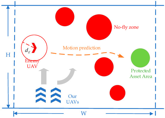
Figure 1.
A schematic diagram of the cooperative pursuit problem of multi-UAVs.
2.2. UAV Model
2.2.1. UAV Motion Model
In this paper, the UAV adopts a particle mass model, and the motion state of the UAV is determined by its position and velocity. The linear acceleration and angular acceleration are used to control the speed and direction of the UAV, achieving agile flight, as shown in Figure 2.
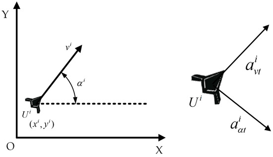
Figure 2.
A schematic diagram of the UAV motion control model.
The instantaneous state information of the UAV at the current time can be represented as follows:
where and represent the position of at time , represents the velocity, represents the heading angle, represents the linear acceleration, represents the angular acceleration, and represents the serial number of the UAV.
So, the instantaneous state information of at time is as follows:
where represents the simulation time step.
2.2.2. UAV Radar Detection and Communication Model
During the mission, the UAVs acquire information through radar detection and communication with each other, as shown in Figure 3.
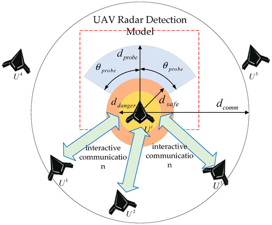
Figure 3.
Schematic diagram of UAV radar detection and intra-swarm communication model.
The detection area of the UAV radar is the fan-shaped area in front of the nose, the maximum detection distance is , and the detection angle is . Considering the constraints of radar tracking performance, the UAV can stably track up to five detection targets at the same time. We set the safe distance and dangerous distance for the UAV. When the distance between the UAV and the detection target is less than the safe distance, there is a collision risk, and the UAV needs to maneuver as soon as possible to avoid obstacles. When the distance between the UAV and the detection target is less than the dangerous distance, the UAV collides and crashes.
The maximum communication distance between the UAV and its teammates is ; considering communication node constraints, each UAV in the team can communicate with up to five teammates at the same time.
2.2.3. Pursuit Model
In the UAV pursuit task, when the target UAV enters our airspace, our UAVs begin to cooperate to pursue the target UAV. The effect of multi-UAVs cooperative rounding up the target is shown in Figure 4.
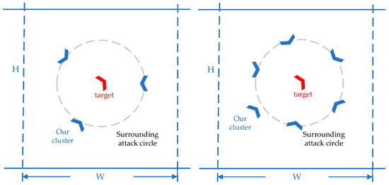
Figure 4.
The effect of multi-UAVs cooperatively rounding up the target.
Figure 4 shows the expected results of a cooperative pursuit with three and six UAVs. Since the maneuverability of the target UAV is better than ours, the basic pursuit strategy is to make our UAVs evenly distributed around the target UAV, forming an encircling situation and increasing the success rate of the pursuit task, as shown in Figure 5.
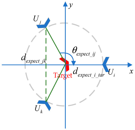
Figure 5.
Diagram of three UAVs completing pursuit task.
As shown in Figure 5, when three UAVs cooperate to perform the pursuit task, the expected distance is shown between our UAVs and the enemy UAV, which is encircled, and our UAVs block the escape path of the target. The angles between the individuals inside the UAVs are evenly distributed according to the number of individuals; so, the expected angle is , ensuring that the UAVs are evenly distributed around the circle.
3. Design of GM-TD3 Algorithm
3.1. Framework of ERL
ERL combines the population-based approach of EAs to generate diverse experiences, train RL agents, and periodically transfer RL agents into EA populations to inject gradient update information into EAs [19]. ERL solves the time credit allocation problem by using the whole round reward. The selection operator tends to choose the policy network with a higher round reward in the policy space based on the fitness index, which is a very effective form of implicit priority ranking for task scenarios with a long time span and sparse rewards. In addition, ERL inherits the characteristics of population-based EAs and has the capability to eliminate any redundancy, which makes the convergence process of the algorithm more stable. ERL takes advantage of a population’s ability to explore in the parameter space and action space, making it easier to generate diversification policies for effective exploration. The basic framework of the ERL algorithm is shown in Figure 6.
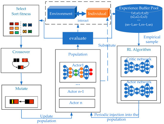
Figure 6.
Diagram of ERL basic framework.
3.2. Genetic Algorithm
In the ERL framework, we choose the genetic algorithm (GA) as the EA. The GA was designed to search for complex solution spaces where an exhaustive search is not feasible and other search methods do not perform well. When used as a function optimizer, the GA tries to maximize the fitness associated with the optimization goal. The GA has been applied to the design and optimization of various problems and has achieved many successful applications [23].
The initial population of the GA is a set of randomly selected valid candidate solutions. The fitness function is used to calculate each individual candidate to obtain the fitness value of the initial population. After the genetic operators of selection, crossover, and mutation are applied, the new generation of individuals is re-evaluated [24,25]. The basic flow of the GA is shown in Figure 7.
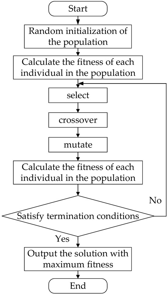
Figure 7.
Diagram of basic flow of GA.
3.3. TD3 Algorithm
In value-based RL algorithms, such as deep Q learning, function approximation errors are known to lead to overestimation and suboptimal strategies, and this problem has been shown to persist in the context of actor–critic algorithm models. The TD3 algorithm is based on double Q learning; by selecting the smaller value of the two estimation functions, it limits the overestimation of the Q value and uses the double-delay update policy to reduce the error of each update, further improving the performance of the algorithm.
The TD3 algorithm consists of six neural networks, namely the “actor_eval” policy estimation network, the “actor_target” policy reality network, the “critic_eval_1” and “critic_eval_2” value estimation networks, and the “critic_target_1” and “critic_target_2” value reality networks. The framework of the TD3 algorithm is shown in Figure 8. In the algorithm, two sets of critic networks are used to evaluate the value of the actor network, and then, the small Q value is selected to update the parameters of the actor network, which can effectively alleviate the problem of overestimation of the Q value. Such improvement may lead to some underestimation, but low estimation will only affect the learning efficiency of training and will not affect the final learning strategy.
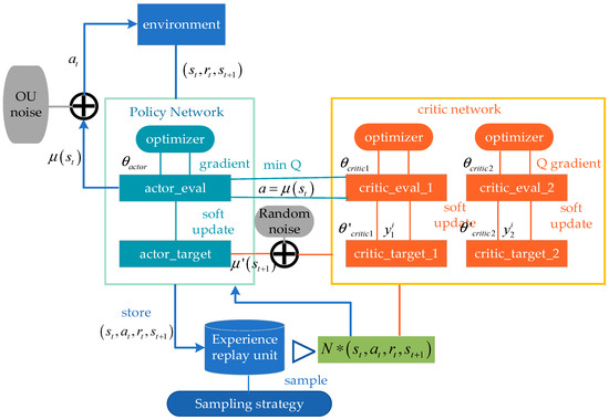
Figure 8.
Diagram of TD3 algorithm framework.
The actor networks take the mean value output of the critic network as the loss function:
Here, is the value assessment of the action behavior output by the critic network for the actor network under the current state, and the minimum value of the two critic networks is used for the calculation.
Critic networks update the network parameters in the value-based mode, and the loss function is as follows:
Here, represents the two critic networks, is the reward that the agent receives after taking action and interacting with the environment in state , is the evaluation of action in state that is output by the “critic_eval_i” network, and is the evaluation of action in state that is output by the “critic_target_i” network.
The network parameters are updated by minimizing the loss functions of the critic_eval and actor_eval networks during training. The network parameters of the critic_target_1, critic_target_2, and actor_target are updated with soft update mode.
3.4. Maximum Mean Discrepancy
As the traditional EA is prone to local optimization, we introduce the MMD method to calculate the difference between the current policy and the elite policy in the population and increase the diversity of policies by gradient updating, thus greatly improving the solution space exploration ability of the algorithm.
Assuming that the elite policy in the current population is , the gradient update of the network parameter of the actor network is in the direction of maximizing the difference between the current policy and , while maximizing the cumulative return. The difference is calculated by using the square of the MMD.
Let us say that given samples and , since the square of the MMD can only be estimated from the sample of a given distribution, then the square of the MMD between distributions P and G is calculated as follows:
Here, is the Gaussian kernel function, as shown below:
In the above equation, is the standard deviation.
The square of the MMD between the elite policy and the policy is denoted as and calculated as follows:
Here, represents the experience sample buffer.
The objective function of the actor network considering the maximization of cumulative returns is as follows:
When satisfies the gradient update, the objective function of the actor network is calculated as follows:
Here, is the weight factor used for regulation.
3.5. Stable Mutation Operator
To improve the stability of the algorithm, a separate individual sample buffer is set for each member of the population and the RL agent, which contains the recent experience of the individual, and depending on its capacity , the buffer can also contain the experience of its parent [26]. Since the buffer can span multiple generations, the individual sample buffer of each agent is referred to as genetic memory.
Even for gradient descent methods, the stability of policy updates is an issue, as inappropriate step sizes can have unpredictable consequences in terms of performance. In this paper, a stable mutation operator is proposed, which first samples a batch of empirical samples from the genetic memory, then calculates the gradient of each dimension of the sample output action, and finally calculates the sensitivity of the samples’ action to the network weight perturbation as follows:
Then, the following formula is used to adjust the network parameters to form a stable mutation operator:
where , and is the variance of the perturbation, such that the behavior of the policy network generated by the variation in the offspring sample does not mutate significantly from that of its parent.
3.6. GM-TD3 Algorithm
The framework design of the GM-TD3 algorithm is shown in Figure 9.
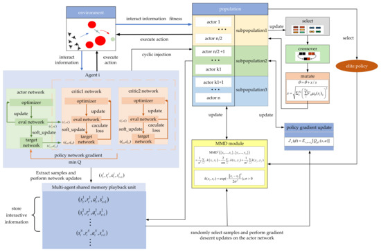
Figure 9.
Framework of GM-TD3 algorithm.
The execution steps of the GM-TD3 algorithm are as follows:
- (1)
- Randomly initialize policy networks as the initial population; randomly initialize the actor networks and critic networks of the TD3 algorithm; randomly initialize the GA algorithm;
- (2)
- Initialize the task scenario, interact the policy network with the environment, and obtain the sample data and store them in the replay buffer ;
- (3)
- Train the TD3 algorithm networks with the sample data;
- (4)
- Interact with the environment to evaluate the strategic populations;
- (5)
- Calculate the fitness values of the individuals in the population and organize the policy network; select the individuals with the highest fitness as the elite strategy ;
- (6)
- Order the individuals in the population based on their fitness values from high to low, and perform cross-mutation on the top K/2 individuals in the sorted population to achieve updates;
- (7)
- Combine the elite strategy and the MMD method to train and update the remaining policy network in the population and generate a new population;
- (8)
- Calculate the fitness of the policy network in the TD3 algorithm and compare it with the worst individual with the lowest fitness in the population; if the policy network of the TD3 algorithm is better than the worst individual in the population, the worst individual will be replaced periodically;
- (9)
- If the algorithm converges or the maximum number of iterations is reached, output the optimal policy network; otherwise, go to (2).
The flowchart of the GM-TD3 algorithm is depicted in Figure 10 and Algorithm 1.
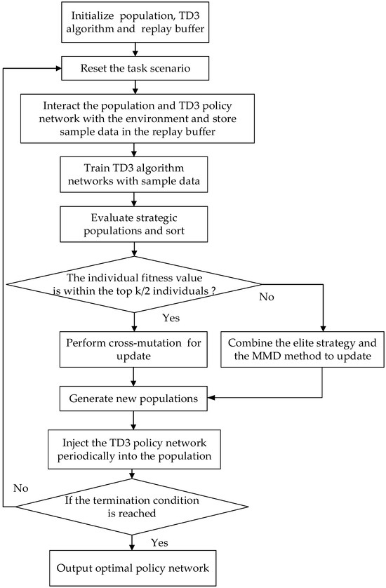
Figure 10.
Flowchart of GM-TD3 algorithm.
The pseudo-code of the GM-TD3 algorithm is as follows:
| Algorithm 1: GM-TD3 |
| Randomly initialize policy networks to generate population , initialize the replay buffer , initialize the maximum number of iterations G, evaluation of round episode M; |
| Initialize the actor network parameters and their target network parameters , and critic1, critic2 network parameters and their target network parameters of the TD3 algorithm; |
| Initialize GA parameters; |
| Construct a noise generator and a random number generator, and define control probability ; |
| While number of iterations n is less than G: |
| For policy network : |
| For evaluation rounds : |
| For steps : |
| Reset environment and initial state ; |
| Select an action based on the current policy network |
| Execute action obtain reward , update to status ; |
| Store in ; |
| Calculate reward = + |
| Set ; |
| End for |
| End for |
| Calculate the fitness of the current policy network: = /; |
| End for |
| Random sample from for training; |
| Update the critic_eval network parameters to minimize losses: |
| Calculate the loss function and obtain the gradient: |
| Update actor_eval network parameters by gradient descent method: |
| If reach the “target” network update period: |
| Update target network parameters using soft update mode; |
| End if |
| Rank the policy network according to the fitness assessed, and select the policy network with the highest fitness as the elite policy ; |
| For policy network : |
| For i = 1 to K/2: |
| The strategy population was cross-mutated to generate progeny and renew the population. |
| End for |
| For i = K/2 + 1 to K1: |
| Samples are extracted from actor networks and update population; |
| Network parameters are updated by gradient descent method: |
| End for |
| For i = K/2 + 1 to K1: |
| Samples are extracted from for training actor networks and update population; |
| Network parameters are updated by gradient descent method: |
| End for |
| End for |
| A new policy population was formed and added to the training process; |
| For policy network : |
| For evaluation rounds : |
| For steps : |
| Reset environment and initial state ; |
| Select an action based on the current policy network ; |
| Execute action , obtain reward , update to status ; |
| Store into ; |
| Calculate reward = + ; |
| Set ; |
| End for |
| End for |
| Calculate the fitness of the current policy network: = /; |
| End for |
| Calculate the fitness of the policy network in TD3 algorithm ; |
| If the policy network of TD3 algorithm outperforms the worst individual in the population: |
| If the number of iterations has reached the update cycle: |
| Replace the worst individual in the population with the policy network in TD3 algorithm; |
| End if |
| End if |
| End while |
4. UAV Pursuit and Escape Game Strategy Based on GM-TD3 Algorithm
4.1. Design of State Space and Action Space
In the multi-UAV cooperative pursuit task, the actions of both sides are trained by the RL method, and the corresponding state space and action space design are shown below.
4.1.1. State Space and Action Space of Our UAVs
The state space of our UAV includes instantaneous state information , target relative position information , and detection information :
The instantaneous state information includes the UAV’s position (, ), speed , and heading angle , as shown below:
As shown in Figure 11, the distance and azimuth angle of relative to the enemy UAV are taken as the target relative position information .
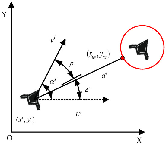
Figure 11.
Relationship between relative positions between UAVs.
Here, is the distance between and the expected rendezvous point, is the azimuth angle of the line between and the expected rendezvous point, and is the azimuth angle of the expected rendezvous point relative to the course of .
To ensure the internal stability and obstacle avoidance ability of the UAVs, five targets’ information which can be stably tracked by the radar of is added into the state space as detection information:
Here, , , , , and are the distance of relative to the detected targets, and , , , and are the azimuth angle of the detected targets relative to . If less than five targets are detected, the corresponding information is set to 0.
Linear acceleration and angular acceleration are used to control the motion of the UAV; so, the action space of is as follows:
4.1.2. State Space and Action Space of Enemy UAV
The state space of the enemy UAV includes instantaneous state information , task information , and detection information :
The instantaneous state information is the same as that of our UAVs.
The objective of the enemy UAV is to avoid the NFZs, evade capture by our UAVs, and complete the attack task on the PA as soon as possible; so, the distance and azimuth angle of the PA relative to the enemy UAV are added to its state space as task information.
Here, and are the distance and azimuth angle between the enemy UAV and the PA; is the azimuth angle of PA relative to the course of enemy UAV.
Similarly, the five targets’ information stably tracked by the radar of the enemy UAV is input into the state space as detection information:
Here, , , , and are the distance of the enemy UAV relative to the detected target, and , , , and are the azimuth angle of the detected target relative to the enemy UAV. If less than five targets are detected, the corresponding information is set to 0.
In the same way, linear acceleration and angular acceleration are used to control the motion of the enemy UAV; so, the action space is as follows:
4.2. Design of Neural Network Structure
In the GM-TD3 algorithm framework, there are two types of neural networks in which the “actor” networks are used to select the actions of the UAVs and output the linear acceleration and angular acceleration of the UAVs to control the motion. The “critic” networks are used to evaluate the value of the actions selected by the “actor” networks and guide the “actor” networks to learn and optimize the policies.
The two types of neural networks are both set as five-layer network structures, and the number of neurons in each layer according to the gradient forward propagation direction is as follows: “actor” networks (64, 128, 256, 128, 2) and “critic” networks (64, 128, 258, 128, 1). In addition to the output layer, the other layers of the neural networks are activated by the ReLU activation function. Considering the requirements of the UAV action space, the output layer is activated by the tanh activation function.
4.3. Design of Reward Function
In the multi-UAV cooperative pursuit task, we set up the mixed-reward function to guide the UAVs to complete their respective tasks according to the task objectives of both sides, as shown below.
4.3.1. Design of Reward Function for Our UAVs
The mixed-reward function of our UAV in the cooperative pursuit task is as follows:
Here, is the individual reward for the UAV, is the global reward for the UAV, is the UAV’s collision reward, is an out-of-bounds reward for the UAV, and are the weight factors.
The individual reward function of the UAV is set as follows:
Here, are the weight factors, is the distance between two adjacent UAVs and , is the expected distance between two adjacent UAVs and , is the distance between UAV and the enemy UAV, and is the expected distance between UAV and the enemy UAV. The individual reward is mainly to reward or punish the trapping situation between the UAV and the target.
The global reward function of the UAV is set as follows:
Here, represents the weight coefficient, while and represent the distance between the UAV and the enemy UAV at time and , respectively. The global reward function mainly evaluates the action of the UAV according to the change in the relative position relationship between our UAV and the enemy UAV.
The collision reward function of the UAV is set as follows:
Here, is the weight coefficient, is the safe distance between adjacent UAVs, and is the current distance between the adjacent UAVs and . The collision reward mainly rewards or punishes the UAV depending on whether it is at a safe distance from the other UAVs.
The out-of-bounds reward of the UAV is set as follows:
Here, are the positions of UAV ; are the length and width of the battlefield. The out-of-bounds reward function mainly rewards or punishes the UAV for flying out of the boundary or not.
4.3.2. Design of Reward Function for Enemy UAV
The mixed-reward function of the enemy UAV in the cooperative pursuit task is as follows:
Here, is the global reward function, is the collision reward function, is an out-of-bounds reward, and are the weight factors.
The global reward function for the enemy UAV is set as follows:
Here, represents the weight coefficient, and and are the distance between the enemy UAV and the PA at time and respectively. The global reward function mainly evaluates the action of the enemy UAV based on the change in the relative position relationship between the enemy UAV and the PA.
The collision reward function and the out-of-bounds reward function of the enemy UAV are the same as those of our UAVs.
5. Simulation Verification
5.1. Training Process
The hardware environment of the simulation platform is as follows: The CPU utilized is the Intel i7-10870H, while the GPU employed is the RTX 3060 manufactured by NVIDIA in Taiwan area, this accelerates the neural network training process. The graphics memory is 6 GB, and the system memory is 32 GB.
The TD3 algorithm and the GM-TD3 algorithm were used for the enemy UAV and our UAVs, respectively, to train the UAVs in the pursuit task scenario, and the initial situation was randomly generated in the task area in each round of algorithm training.
The major parameter settings are shown in Table 1.

Table 1.
Training parameters for multi-UAV pursuit task.
In the training process of the two algorithms, the mean value and variance of the weight parameters in the “actor_eval” neural network change with the training rounds, as shown in Figure 12.
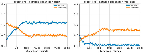
Figure 12.
Mean and variance change curve of actor_eval neural network parameters during training.
As can be seen in figure, during the training process of our UAVs using the GM-TD3 algorithm, because the GA is used to optimize the population of the policy network and the MMD method is used to increase the exploration space of the policy, the fluctuation in the update of the neural network parameters is more stable during training, and the convergence speed of the algorithm is significantly accelerated. With the increase in training rounds, the parameters of the neural networks can converge to the stationary state faster. The convergence and stability of our UAVs are obviously better than that of the enemy UAVs, and the trained policy network can better complete the pursuit task.
We record the individual reward value of both the enemy and our UAVs under each training round in the algorithm training process, as shown in Figure 13.
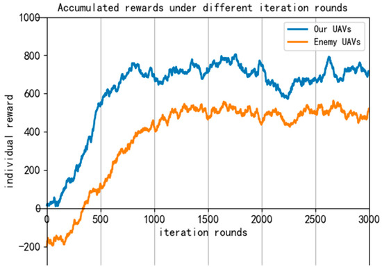
Figure 13.
Reward curve during algorithm training.
It can be seen from the reward curve that as the training epochs increase, the reward values of both sides gradually rise. At about 900 epochs, the reward value of both sides levels off and our UAVs gradually achieve the encirclement pursuit task of the enemy UAV. This shows that the improved algorithm is effective in the UAV pursuit task.
5.2. Verification Process
We use the trained GM-TD3 and TD3 algorithm models for simulation verification to test the effectiveness of the algorithm. In the simulation task scenario, the PA is represented by a green circular area, the red circular areas are the NFZs, our UAVs are shown in blue, and the enemy UAV is shown in red. The snapshot of the simulation effect for the 3vs1 pursuit game task is shown in Figure 14. The red areas indicate no-fly zones (NFZ), while the blue areas represent protected asset areas.
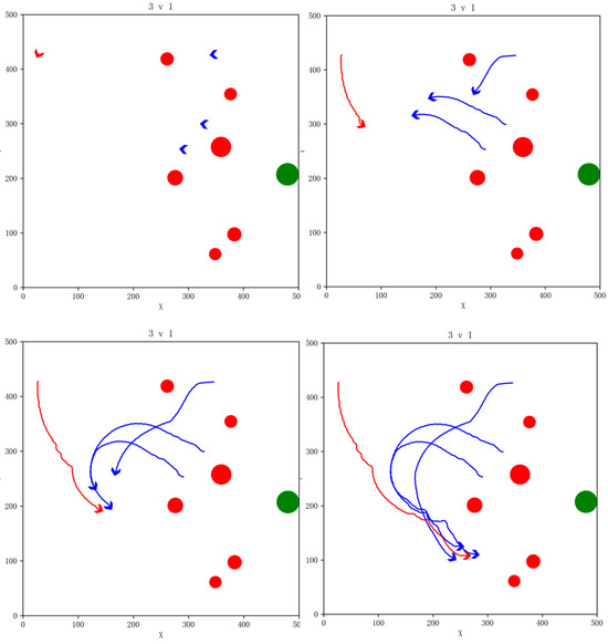
Figure 14.
Snapshot of simulation effects for 3vs1 pursuit game task with NFZs.
In the simulation, our three UAVs successfully evaded the NFZs and coordinated to round up the enemy UAV. The enemy UAV carried out avoidance maneuvers while evading the NFZs and finally were surrounded by our UAVs and failed to reach the PA. Our UAVs successfully completed the pursuit task.
In order to validate the simulation performance and generalization capability of the algorithm under various conditions, we varied the number of our UAVs and no-fly zones, randomly generated the initial states of the drones, and carried out simulation verification in the 4vs1 and 6vs1 task scenarios; our UAVs were able to successfully complete the pursuit task. The snapshot of the simulation effects is shown in Figure 15 and Figure 16.
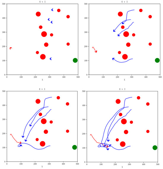
Figure 15.
Snapshot of simulation effects for 4vs1 pursuit game task with 10 NFZs.
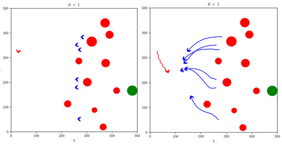
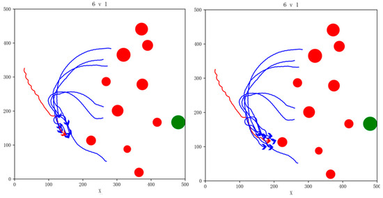
Figure 16.
Snapshot of simulation effects for 6vs1 pursuit game task with 10 NFZs.
In order to further verify the generalization ability of the GM-TD3 algorithm, we conducted a simulation of the task scenario without NFZs. The simulation effect for the 3vs1 task scenario is shown in Figure 17. Our UAVs successfully completed the pursuit task. As can be seen from the simulation effect, in the task scenario without NFZs, the enemy UAV is less restricted, so it is easier to exert its maneuvering ability advantage and pose a greater threat to our PA.
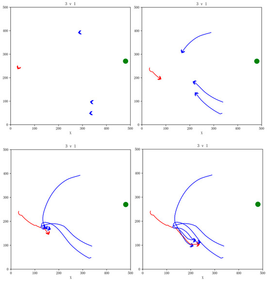
Figure 17.
Snapshot of simulation effects for 3vs1 pursuit game task without NFZs.
5.3. Algorithm Comparison and Analysis
We used the TD3, GA-TD3 (TD3 algorithm combining ERL with GA, GA-TD3), and GM-TD3 algorithms to train our UAVs and the TD3 algorithm to train the enemy UAV to compare the performance advantages of the algorithms.
In the training process of 3000 rounds, the individual reward curve of our UAV is shown in Figure 18. It can be seen that the overall convergence trend of the three algorithms is roughly the same, but the convergence speed of the GM-TD3 algorithm is faster; it can obtain higher global rewards, and it has obvious performance advantages.
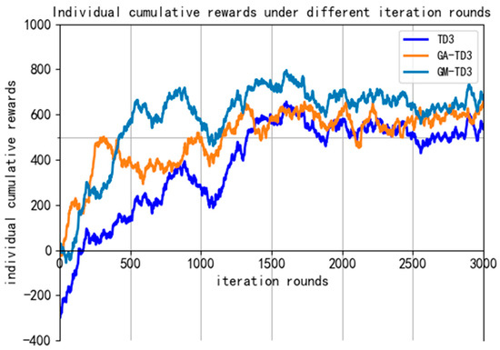
Figure 18.
The global reward curve of the three algorithms.
The task success rates of the three algorithms in different training rounds are shown in Figure 19.
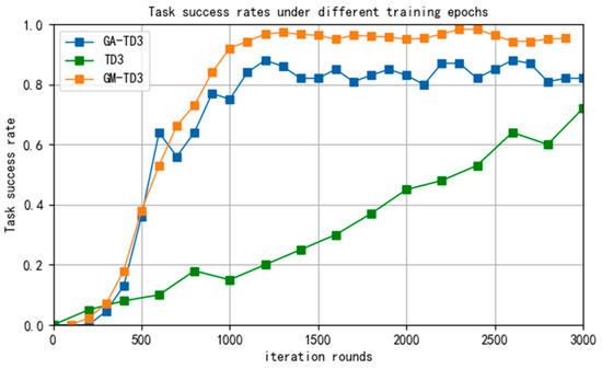
Figure 19.
The task success rates of the three algorithms.
It can be seen that the task success rate of the GA-TD3 and GM-TD3 algorithms has significantly improved after 1000 rounds of training and basically reached stability after 2000 rounds of training. Through a large number of simulations, the task success rate of the GM-TD3 algorithm is stable at about 95% and that of the GA-TD3 algorithm is about 85%. However, the success rate of the TD3 algorithm has been maintained at a low level, and it is difficult to achieve the pursuit task against an enemy UAV with a speed advantage. Therefore, the task success rate and the convergence rate of the GM-TD3 algorithm are better than those of the GA-TD3 and TD3 algorithms, which shows the superiority of the improved algorithm.
To verify the effect of the speed advantage of enemy UAVs on the performance of the GM-TD3 algorithm, the task success rates of the TD3, GA-TD3, and GM-TD3 algorithms were simulated under different maximum UAV speed ratio constraints. The simulation results are shown in Figure 20; in the figure, the horizontal coordinate represents the ratio of the maximum speed of the enemy UAV to our UAV, and the vertical coordinate represents the task success rate.
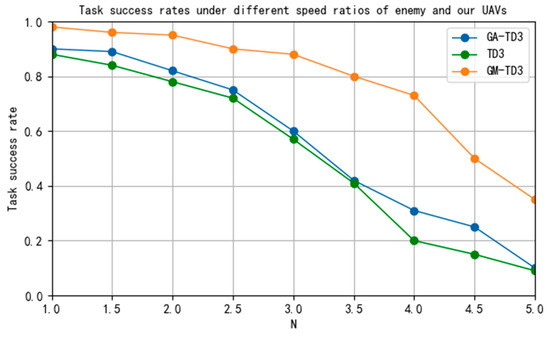
Figure 20.
Task success rate under different UAV maximum speed ratios.
6. Conclusions
This paper focuses on the task of multi-UAV cooperative pursuit of a high-speed enemy UAV. We improve the traditional TD3 algorithm, combine the algorithm with the GA-based ERL framework, and introduce the MMD method to expand the space for algorithm policy exploration. The improved algorithm can effectively improve the exploration efficiency of the policy space and the training efficiency of the algorithm. Through a large number of simulation experiments, we verify that the performance of the improved GM-TD3 algorithm has been greatly improved and it can achieve faster convergence compared with the GA-TD3 and TD3 algorithms. With an enemy UAV four times as fast as ours, the task success rate can still reach 75%; however, the task success rate of the GA-TD3 and TD3 algorithms under the same conditions is lower than 35%, which indicates that the improved GM-TD3 algorithm has better ability to execute cooperative pursuit tasks, especially for high-speed enemy UAVs.
Future research directions will primarily focus on the limitations of the algorithm proposed in this paper when applied to other scenarios, particularly in the context of multi-target evasion. This involves designing pursuit–evasion game scenarios that include multiple hostile escaping drones and multiple friendly drones. Further improvements will be made to the GM-TD3 algorithm introduced in this paper, with particular attention paid to the dynamic allocation of targets during the pursuit process, as well as enhancing the intelligence, generalizability, and realism of the scenarios, extending the improvements to a 3D environment.
Author Contributions
Conceptualization, Y.Z.; methodology, M.D.; software, Y.Y.; validation, M.D., Y.Y. and J.Z.; formal analysis, Q.Y.; investigation, G.S.; resources, F.J.; data curation, M.D. and M.L.; writing—original draft preparation, Y.Z.; writing—review and editing, J.Z., Q.Y., G.S., F.J. and M.L.; visualization, M.D. and Y.Y.; supervision, Y.Z.; project administration, J.Z., F.J. and M.L.; funding acquisition, Y.Z. and M.L. All authors have read and agreed to the published version of the manuscript.
Funding
This work was supported by the Aeronautical Science Foundation of China under the grant number 20220013053005 and in part by the Basic Scientific Research Ability Improvement Project for Middle-young Teachers under the grant number 2024KY0173.
Data Availability Statement
Dataset available on request from the authors.
Conflicts of Interest
The authors declare no conflict of interest.
References
- Liu, D.; Zhai, J.; Wei, L.; Guo, M.; Lin, S.; Huang, P.; Wang, X. UAV Cluster Task Planning and Collaborative System Architecture. Acta Armamentarii 2024. [Google Scholar] [CrossRef]
- Bi, W.H.; Zhang, M.Q.; Gao, F.; Yang, M.; Zhang, A. Review on UAV swarm task allocation technology. Syst. Eng. Electron. 2024, 46, 922–934. [Google Scholar]
- Li, J.; Chen, S.C. Review of Key Technologies for Drone Bee Colony Development. Acta Armamentarii 2023, 44, 2533–2545. [Google Scholar]
- Gong, Y.Q.; Zhang, Y.P.; Ma, W.P.; Xue, X. The mechanism of swarm intelligence emergence in drone swarms. Acta Armamentarii 2023, 44, 2661–2671. [Google Scholar]
- He, F.; Yao, Y. Maneuver decision-making on air-to-air combat via hybrid control. In Proceedings of the IEEE Aerospace Conference, Big Sky, MT, USA, 6–13 March 2010; pp. 1–6. [Google Scholar]
- Liu, X.Y.; Guo, R.H.; Ren, C.C.; Yan, C.; Chang, Y.; Zhou, H.; Xiang, X.J. Distributed target allocation method for UAV swarms based on identity-based Hungarian algorithm. Acta Armamentarii 2023, 44, 2824–2835. [Google Scholar]
- Zhao, L.; Cong, L.; Guo, X. Research of cooperative relief strategy between government and enterprise based on differential game. Syst. Eng. Theory Pract. 2018, 38, 885–899. [Google Scholar]
- Fu, L.; Wang, X.G. Research on differential game modeling for close range air combat of unmanned aerial vehicles. Acta Armamentarii 2012, 33, 1210–1216. [Google Scholar]
- Li, Y.L.; Li, J.; Liu, C.; Li, J. Research on the Application of Differential Games in the Attack and Defense of Drone Clusters. Unmanned Syst. Technol. 2022, 5, 39–50. [Google Scholar]
- Huang, H.Q.; Bai, J.Q.; Zhou, H.; Cheng, H.Y.; Chang, X.F. The Development Status and Key Technologies of Unmanned Collaborative Warfare under Intelligent Air Warfare System. Navig. Control 2019, 18, 10–18. [Google Scholar]
- Wen, Y.M.; Li, B.Y.; Zhang, N.N.; Li, X.J.; Xiong, C.Y.; Liu, J.X. Multi agent formation collaborative control based on deep reinforcement learning. Command. Inf. Syst. Technol. 2023, 14, 75–79. [Google Scholar]
- Lowe, R.; Wu, Y.I.; Tamar, A.; Harb, J.; Pieter Abbeel, O.; Mordatch, I. Multi-Agent Actor-Critic for Mixed Cooperative-Competitive Environments. arXiv 2018, arXiv:1706.02275v3. [Google Scholar]
- Hao, J.; Huang, D.; Cai, Y.; Leung, H.F. The dynamics of reinforcement social learning in networked cooperative multiagent systems. Eng. Appl. Artif. Intell. 2017, 58, 111–122. [Google Scholar] [CrossRef]
- Fang, M.; Groen, F.C.A. Collaborative multi-agent reinforcement learning based on experience propagation. J. Syst. Eng. Electron. 2013, 24, 683–689. [Google Scholar] [CrossRef][Green Version]
- Van Moffaert, K.; Nowé, A. Multi-objective reinforcement learning using sets of pareto dominating policies. J. Mach. Learn. Res. 2014, 15, 3483–3512. [Google Scholar]
- Wu, F.G.; Tao, W.; Li, H.; Zhang, J.W.; Zheng, C.C. Intelligent Obstacle Avoidance Decision-Making for Drones Based on Deep Reinforcement Learning Algorithms. Syst. Eng. Electron. 2023, 45, 1702–1711. [Google Scholar]
- Phadke, A.; Medrano, F.A.; Chu, T.; Sekharan, C.N.; Starek, M.J. Modeling Wind and Obstacle Disturbances for Effective Performance Observations and Analysis of Resilience in UAV Swarms. Aerospace 2024, 11, 237. [Google Scholar] [CrossRef]
- Tu, G.T.; Juang, J.G. UAV path planning and obstacle avoidance based on reinforcement learning in 3d environments. Actuators 2023, 12, 57. [Google Scholar] [CrossRef]
- Khadka, S.; Tumer, K. Evolution-guided policy gradient in reinforcement learning. In Proceedings of the Advances in Neural Information Processing Systems, Vancouver, BC, Canada, 3–8 December 2018; Volume 31. [Google Scholar]
- Pourchot, A.; Sigaud, O. CEM-RL: Combining evolutionary and gradient-based methods for policy search. arXiv 2018. [Google Scholar] [CrossRef]
- Zheng, H.; Wei, P.; Jiang, J.; Long, G.; Lu, Q.; Zhang, C. Cooperative heterogeneous deep reinforcement learning. In Proceedings of the Advances in Neural Information Processing Systems, Vancouver, BC, Canada, 6–12 December 2020; pp. 17455–17465. [Google Scholar]
- Tjanaka, B.; Fontaine, M.C.; Togelius, J.; Nikolaidis, S. Approximating gradients for differentiable quality diversity in reinforcement learning. In Proceedings of the Genetic and Evolutionary Computation Conference, Boston, MA, USA, 9–13 July 2022; pp. 1102–1111. [Google Scholar]
- Wei, T.; Long, C. Path planning of mobile robots based on improved genetic algorithm. J. Beijing Univ. Aeronaut. Astronaut. 2020, 46, 703–711. [Google Scholar] [CrossRef]
- Dankwa, S.; Zheng, W. Twin-delayed ddpg: A deep reinforcement learning technique to model a continuous movement of an intelligent robot agent. In Proceedings of the 3rd International Conference on Vision, Image and Signal Processing, Vancouver, BC, Canada, 26–28 August 2019; pp. 1–5. [Google Scholar]
- Jiang, F.Q.; Chen, Z.L.; Gao, X.J.; Zhang, Y. Research on Drone Area Reconnaissance Based on an Improved TD3 Algorithm. Informatiz. Res. 2023, 49, 36–42. [Google Scholar]
- Zhao, C.; Liu, Y.G.; Chen, L.; Li, F.Z.; Man, Y.C. Current situation and prospect of multi-UAV path planning for metaheuristic algorithms. Control. Decis. 2022, 37, 1102–1115. [Google Scholar]


Disclaimer/Publisher’s Note: The statements, opinions and data contained in all publications are solely those of the individual author(s) and contributor(s) and not of MDPI and/or the editor(s). MDPI and/or the editor(s) disclaim responsibility for any injury to people or property resulting from any ideas, methods, instructions or products referred to in the content. |
© 2024 by the authors. Licensee MDPI, Basel, Switzerland. This article is an open access article distributed under the terms and conditions of the Creative Commons Attribution (CC BY) license (https://creativecommons.org/licenses/by/4.0/).