Grid Matrix-Based Ground Risk Map Generation for Unmanned Aerial Vehicles in Urban Environments

Abstract

As a novel mode of urban air mobility (UAM), unmanned aerial vehicles (UAVs) pose a great amount of risk to ground people. Assessing ground risk and mitigation effects correctly is a focused issue. This paper proposes a grid-based risk matrix framework for assessing the ground risk associated with two types of UAVs, namely fixed-wing and quadrotor. The framework has a three-stage structure of “intrinsic risk assessment—mitigation effect—final map generation”. First, the intrinsic risk to ground populations caused by potential UAV crashes is quantified. Second, the mitigation effects are measured by establishing a mathematical model with a focus on the ground sheltering and parachute systems. Finally, a modular approach is presented for generating a ground risk map of UAVs, aiming to effectively characterize the effects of each influencing factor on the failure process of UAVs. The framework facilitates the modular analysis and quantification of the impact of diverse risk factors on UAV ground risk. It also provides a new perspective for analyzing ground risk mitigation measures, such as ground sheltering and UAV parachute systems. A case study experiment on a realistic urban environment in Shenzhen shows that the risk map generated by the presented framework can accurately characterize the distribution of ground risk posed by various UAVs.

1. Introduction

The advancement of technologies and applications of unmanned aircraft vehicles (UAVs) earns increasing attention on urban air mobility (UAM) [1,2]. Many conventional logistics and start-up companies are actively developing UAV business lines, with a focus on last-mile delivery. Amazon initiated research into UAV delivery services in 2013 and obtained the FAA Part 135 air carrier operating certificate in 2020 [3]. MeiTuan (a technology-driven retail company) has started using UAVs to deliver food in certain areas of Shenzhen, China [4]. Antwork (a start-up company) is dedicated to building an urban aerial logistics network and was granted the first urban logistics operation license by the Civil Aviation Administration of China (CAAC) in 2019 [5].

Joint Authorities for Rulemaking of Unmanned Systems (JARUS) issued guidelines for the Special Operations Risk Assessment (SORA) process for specific types of UAVs [6]. These guidelines state that UAV operations must be maintained at an acceptable risk level, particularly in densely populated urban environments. Although there is substantial demand for UAV applications in urban transportation scenarios, these areas pose a high risk to UAV operations. Reference [7] presented a UAV spectrum monitoring approach based on deep learning, which provides fundamental data for the safety surveillance of urban airspace.

How to assess the ground risk caused by UAV failures becomes a key for UAV operations. The core focus lies in evaluating the impacts of UAV operations on urban ground populations and the effectiveness of protective measures. In the military domain, the U.S. military introduced a “kill box” model [8], which involves planning a three-dimensional space above a target area based on a global grid to simulate air-to-ground strike effects. This model has been adopted and adapted in subsequent studies. A significant portion of previous research is based on probabilistic models that analyze the impact of UAV ground collisions. Zhang [9] considered the fatality rate resulting from UAV crashes, incorporating different types of UAV parameters and ground population data to calculate the casualty area and the probability of fatal ground injuries in real scenarios. Hu [10] proposed a comprehensive risk assessment model for UAV operations in urban environments considering three categories of risk, which are humans, vehicles, and manned aircraft. Li [11] introduced a city environment model that incorporates safety margins, allowing UAVs to maintain a safe distance from urban structures. They also developed a risk assessment model for the impact of UAV paths on ground personnel. Han [12] used over 20,000 flight hours of operational data to establish a Bayesian network-based risk assessment model to identify the primary failure causes of accidents and proposed mitigation measures to reduce the UAV risks to 3.84 × 10⁻⁸. In their subsequent work [13], they continued to explore the impact of UAV flight path errors on ground risk assessment. Zhang [14] formulated a ground impact model to ascertain the Target Levels of Safety (TLOS) for UAV systems, evaluating these levels across various scenarios and different types of UAVs. Bu [15] proposed a risk assessment and quantification method based on K-means clustering, which constructed indicators for both aerial and ground risk. Cour-Harbo [16,17] analyzed four different crash modes following UAV system failures and discussed the influence of UAV parameters and wind speed on the fall trajectory under ballistic descent mode. Du [18] provided a detailed review and summary of the recent research on UAV risk assessment.

Referring to the ground risk map generation, Primatesta [19,20,21] proposed a risk-aware path planning strategy for UAVs in urban environments, utilizing risk maps to associate discrete spatial locations with corresponding risk costs. In collaboration with Cour-Harbo [22], they created a comprehensive risk map by integrating layers such as population density, obstacles, sheltering, and no-fly zones with four different UAV failure modes. Li [23] generated a risk map by dividing a risk grid into three independent layers, which are the risk, obstacles, and special zones. Pang and Hu [24] introduced a comprehensive risk assessment model for UAV path planning incorporating the casualty risk, property damage risk, and noise impact. For dynamic risk maps, Aliaksei [25] utilized the spatiotemporal population density data to assess ground risk posed by UAVs. Jiao [26] addressed the issue of dynamic population density distribution by proposing a dynamic model that combines Long Short-Term Memory (LSTM) networks and a dynamic model to predict ground risk, validating the spatiotemporal characteristics of these risks. Pang [27] proposed a dynamic ground risk assessment method based on population density prediction. Ye [28] used a two-dimensional (2D) grid to represent the ground risk of UAVs for path planning. Zhang [29] constructed a three-dimensional (3D) risk assessment matrix to express the impact of UAVs on ground individuals and vehicles. Studies [30,31] have also utilized a 2D/3D risk matrix to depict the ground risk of UAVs for safe path planning in discrete airspace.

Although these studies consider a wide range of risk factors, these factors are often interlinked and cascaded, leading to a lack of a modular assessment framework that can quantitatively evaluate the actual impact of various risk factors. In addition, these studies often lack the consideration of the realistic urban environments and do not analyze the effectiveness of ground risk mitigation measures for different types of UAVs from a broader, wide-area perspective. These disadvantages may lead to the overestimation of the risk.

This paper presents a framework to tackle the issues mentioned above. The first modular in the framework is developing a ground risk assessment method for UAV operations. A matrix-based framework is proposed to enable a separate characterization of the effects of various risk factors. Second, a risk reduction with parachute systems is analyzed. How this reduction mechanism affects the ground risk is given. In the end, a method of generating a ground risk map is proposed by incorporating the urban airspace structure and corresponding attributes.

The rest of the paper is structured as follows: Problem description is given in Section 2. The analysis of ground risk factors is described in Section 3. The ground risk map generation method is proposed in Section 4. The case study for validation is shown in Section 5. Finally, the paper is concluded in Section 6.

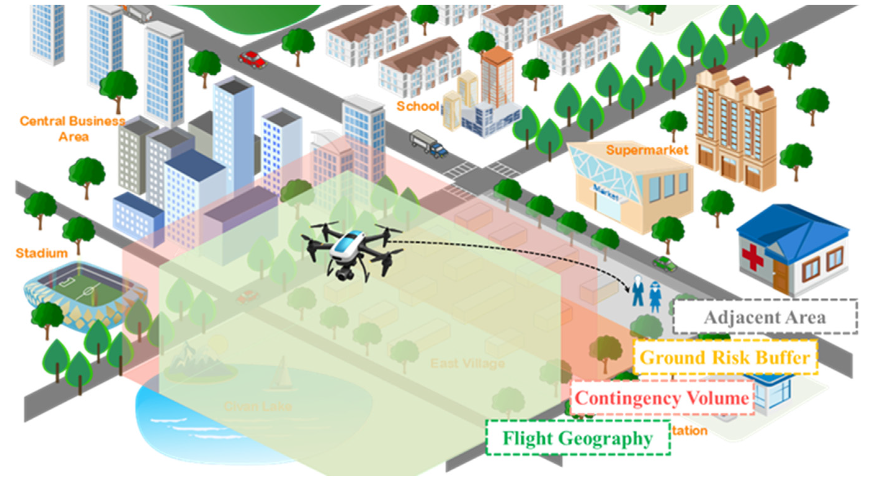
2. Problem Description

A ground risk map belongs to a two-dimensional geographic grid-based map that requires the selection of an appropriate resolution based on the population distributions. The ground risk of each grid should be calculated. The three-stage framework of “intrinsic risk assessment—mitigation effect—final map generation” proposed in this paper is illustrated in Figure 1.

First, a resolved geographic grid is selected appropriately. Then, the ground impact locations and casualty areas are derived by using corresponding UAV-specific parameters, ground population density, and UAV failure and crash models. This allows for the calculation of the intrinsic ground risk matrix imposed by UAV operations. In the second step, based on the three-dimensional urban airspace structure, the protective effects of the UAV parachute systems and various urban environment sheltering features are considered. These risk reduction effects are calculated accordingly. Finally, a modular analysis of the effects provided by different risk mitigation measures is conducted using matrix forms, which further constructs a ground risk mitigation matrix. This matrix is used to derive the final ground risk matrix for the UAVs. A ground risk map is generated by integrating both the airspace structure layer and no-fly zone layer.

3. Derivation of Ground Risk Factors

The current section explains the origin of ground risk associated with UAVs and examines the physical process of risk mitigation measures based on the kinematic theory in Section 3.2. In particular, all the derivations in Section 3.2.2 are based on kinematic equations and can be obtained through calculus. These findings will play a crucial role in determining the final ground risk matrix in Section 4.

3.1. Intrinsic UAV Ground Risk Matrix

A ground risk map is a two-dimensional geographic grid-based map that divides an urban area into multiple grids, which is shown in Figure 2. Risk assessment is implemented for each ground grid by quantifying its population density and building distribution in each grid. The ground grids are typically defined squares, and their risk levels represent the potential casualties caused by a UAV crash in that area. It can be expressed as a risk matrix. In this paper, a risk matrix is defined as ${\mathit{R}}_{m\times n}$ with a size of $m\times n$ which is given in Figure 2. Each element $R(i,j)$ in this risk matrix ${\mathit{R}}_{m\times n}$ represents the risk value of the corresponding ground grid.

For any geographic location $(x,y)$ within a ground risk map of range $X\times Y$, the relationship between a geographic grid $R_{\mathrm{map}}(x,y)$ and a matrix element $R_{\mathrm{mat}}(i,j)$ can be established using a simple coordinate transformation as given in Equations (1) and (2). Here, in these equations, $r$ represents the resolution of a geographic grid.

$$\left\{\begin{array}{c}i=⎣\frac{x}{r}⎦,\\ j=⎣\frac{y}{r}⎦.\end{array}\right.$$

(1)

$$\left\{\begin{array}{c}r\cdot n=X,\\ r\cdot m=Y.\end{array}\right.$$

(2)

The intrinsic ground risk is an inherent attribute of UAV operations depending on the UAV’s characteristics including the maximum dimension, maximum takeoff weight, and cruising speed. The population density of the crashed area is also indispensable [6]. In this way, an intrinsic ground risk matrix ${\mathit{R}}_{\mathrm{i}}$ for UAV operations can be expressed as Equation (3),

$${\mathit{R}}_{\mathrm{i}}=\left[\begin{array}{cccc}{R}_{\mathrm{i}}(1,1)& R_{\mathrm{i}}(1,2)& \cdots & R_{\mathrm{i}}(1,n)\\ R_{\mathrm{i}}(2,1)& R_{\mathrm{i}}(2,2)& \cdots & R_{\mathrm{i}}(2,n)\\ ⋮& ⋮& & ⋮\\ R_{\mathrm{i}}(m,1)& R_{\mathrm{i}}(m,2)& \cdots & R_{\mathrm{i}}(m,n)\end{array}\right].$$

(3)

As illustrated in Figure 3, a UAV crosses the boundary of a contingency volume, passes through a ground risk buffer, and crashes in an adjacent area. The ground risk of this UAV’s crash can be computed using Equation (4) according to the SORA V2.5 Annex F [32].

$$E_{\mathrm{C},\mathrm{adj}}=P(\mathrm{ADJ})\cdot P(\mathrm{GI}|\mathrm{ADJ})\cdot D_{\mathrm{popavg},\mathrm{adj}}\cdot A_{\mathrm{C},\mathrm{unmit}}\cdot {10}^{M_{1,\mathrm{adj}}+M_{2,\mathrm{adj}}},$$

(4)

where $E_{\mathrm{C},\mathrm{adj}}$ represents the expected casualty per hour resulting from a UAV crash in the adjacent area. $P(\mathrm{ADJ})$ denotes the probability of a UAV entering the adjacent area. $P\left(\mathrm{GI}\right|\mathrm{ADJ})$ indicates the probability of a UAV experiencing a loss of control and crashing on the ground in the adjacent area. $D_{\mathrm{popavg},\mathrm{adj}}$ represents the population density of the adjacent area. $A_{\mathrm{C},\mathrm{unmit}}$ is the casualty area covered by the UAV’s crash, and ${10}^{M_{1,\mathrm{adj}}+M_{2,\mathrm{adj}}}$ is the risk reduction value brought by some ground risk mitigation measures. $M_{1,\mathrm{adj}}$ and $M_{2,\mathrm{adj}}$ represent the effects of the M1-type and M2-type ground risk mitigation measures, respectively [33]. These measures will be introduced in Section 3.2.

The ground casualties caused by the UAV’s crash can be categorized into two types, which are sharp force injuries and blunt force injuries [34]. The former, sharp force injuries, generally refer to the harm caused by the UAV’s propellers or other sharp edges, while the latter, blunt force injuries, are due to the kinetic energy of the UAV via the impact. This study focuses exclusively on the assessment of the UAV impact injuries from blunt force trauma.

If the UAV has crossed the ground buffer and crashed in the adjacent area, with the ground population fully exposed within the casualty area, then $P(\mathrm{ADJ})=1$ and $P\left(\mathrm{GI}\right|\mathrm{ADJ})=1$. Assume that $P_{\mathrm{f}}={10}^{M_{1,\mathrm{adj}}+M_{2,\mathrm{adj}}}$; omitting risk mitigation measures, Equation (4) can be simplified as

$$E_{\mathrm{C},\mathrm{adj}}=D_{\mathrm{popavg},\mathrm{adj}}\cdot A_{\mathrm{C},\mathrm{unmit}}\cdot P_{\mathrm{f}},$$

(5)

where $P_{\mathrm{f}}$ is the fatality rate curve for human impact from UAVs, as proposed by Dalamagkidis [35]. $P_{\mathrm{f}}$ can be calculated with Equation (6),

$$P_{\mathrm{f}}={\displaystyle \frac{1-k}{1-2k+\sqrt{\frac{\alpha }{\beta }}\cdot {(\frac{\beta }{E_{\mathrm{crash}}})}^{\frac{3}{P_{\mathrm{s}}}}}}.$$

(6)

The ground sheltering parameter $P_{\mathrm{s}}$ determines the level of population exposure to an impact. $\alpha$ is the impact energy required for a fatality probability of 50% when $P_{\mathrm{s}}=6$, and $\beta$ is the impact energy threshold required to cause a fatality as $P_{\mathrm{s}}$ goes to zero. According to [9,22,35,36], $\alpha$ and $\beta$ are set to be 34 kJ and 34 J, respectively. $E_{\mathrm{crash}}$ represents the kinetic energy of the UAV at the moment of impact, which is calculated using Equation (7) according to the theorem of kinetic energy. The correction factor $k$ can be computed using Equation (8), and can be used to improve the estimates given for low kinetic energies, particularly those approaching or falling below the threshold limit of 34 J.

$$E_{\mathrm{crash}}={\displaystyle \frac{1}{2}}m\cdot ||{\mathit{v}}_{\mathrm{c}}|{|}^2,$$

(7)

$$k=\min \left[1,{({\displaystyle \frac{\beta }{E_{\mathrm{crash}}}})}^{{\displaystyle \frac{3}{P_{\mathrm{s}}}}}\right],$$

(8)

where $m$ represents the mass of the UAV and ${\mathit{v}}_{\mathrm{c}}$ denotes the instantaneous velocity of the UAV at the moment of impact. The ground sheltering parameter approaches zero ($P_{\mathrm{s}}\to 0$) when the ground population is fully exposed to the UAV crash risk without protective mitigation measures. The fatality rate associated with the UAV impact at this time is contingent upon the magnitude of the impact kinetic energy.

$$P_f=\left\{\begin{array}{cc}0& E_{\mathrm{crash}}\le \beta ,\\ 1& E_{\mathrm{crash}}\ge \beta .\end{array}\right.$$

(9)

$R_{\mathrm{i}}(i,j)$ is used to represent the intrinsic ground risk of the UAV impact for each risk unit $(i,j)$ within the grid risk matrix, leading to the derivation of Equation (10).

$$R_{\mathrm{i}}(i,j)=\left\{\begin{array}{ll}0\hfill & E_{\mathrm{crash}}\le \beta ,\hfill \\ D_{\mathrm{p}}(i,j)\cdot A_{\mathrm{c},\mathrm{b}}\hfill & E_{\mathrm{crash}}>\beta ,\hfill \end{array}\right.$$

(10)

where $D_{\mathrm{p}}(i,j)$ is the population density associated with the risk cell’s location $(i,j)$, and $A_{\mathrm{c},\mathrm{b}}$ represents the casualty area of the UAV impact within the ballistic descent model. In this paper, the UAV is influenced solely by gravitational and drag forces, following a ballistic descent trajectory. The ballistic descent model employs a standard second-order drag framework extensively developed by La Cour-Harbo in [16], and $A_{\mathrm{c},\mathrm{b}}$ can be calculated with Equations (11) and (12) using methodologies in references [9,22].

$$A_{\mathrm{c},\mathrm{b}}=2(r_{\mathrm{p}}+r_{\mathrm{u}})d_{\mathrm{b}}+\pi {(r_{\mathrm{p}}+r_{\mathrm{u}})}^2,$$

(11)

$$d_{\mathrm{b}}=h_{\mathrm{p}}{\displaystyle \frac{\left|{\mathit{v}}_{\mathrm{c},\mathrm{b}}^x\right|}{\left|{\mathit{v}}_{\mathrm{c},\mathrm{b}}^y\right|}}.$$

(12)

In this context, $r_{\mathrm{p}}$ and $h_{\mathrm{p}}$ denote the average radius and height of an individual, respectively, and $r_{\mathrm{u}}$ signifies the average radius corresponding to the largest size of the UAV. These parameters are treated as constants. The variable $d_{\mathrm{b}}$ represents the impact distance of the UAV upon ground contact, which is inversely related to its approach angle at crashing. This relationship can be articulated through the horizontal and vertical velocities of the UAV at impact, denoted as ${\mathit{v}}_{\mathrm{c},\mathrm{b}}^x$ and ${\mathit{v}}_{\mathrm{c},\mathrm{b}}^y$, respectively, utilizing a ballistic descent model. The terminal motion of the UAV during ground contact is approximated as linear motion, and solved by Equation (12).

3.2. Ground Risk Mitigation Effects

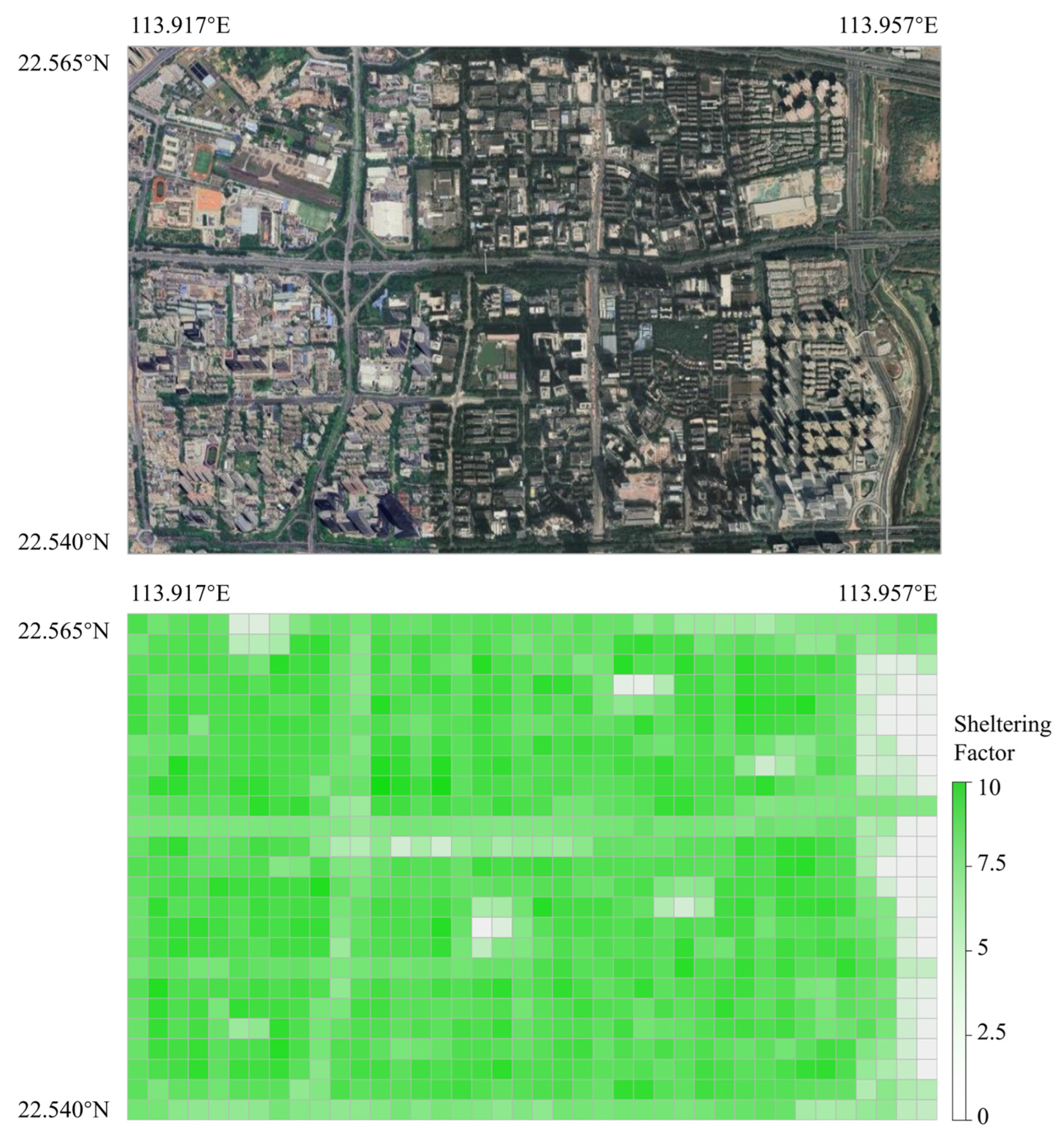
3.2.1. Ground Sheltering Effects

The intrinsic ground risk represents the most immediate safety concern associated with a UAV crashing into populated areas. However, the ground risk level can be reduced by adopting mitigation strategies in SORA [6,32]. As delineated in Annex B of SORA [33], these measures are classified into two types: M1 and M2. The primary aim of the M1 measure is to minimize the number of individuals that are directly exposed within the risk area. For the M1 measure, the ground sheltering parameter serves as an effective metric for quantifying the benefits derived from risk mitigation through ground sheltering under some typical conditions. This paper exclusively examines the protective impact of the ground sheltering parameter $P_{\mathrm{s}}$ with Equation (6) illustrating its effect on fatality rates on the ground due to UAV incidents. $P_{\mathrm{s}}$ is influenced by the ground characteristics such as buildings or trees that can significantly attenuate the kinetic energy when UAVs impact and thereby, the probability of fatality can be reduced.

$$P_{\mathrm{s}}={\displaystyle \sum _{i=1}^j{P}_{\mathrm{s}}^i\cdot \frac{S_i}{S}},$$

(13)

Equation (13) delineates a methodology for calculating the ground sheltering parameter for each grid on the ground, where $P_{\mathrm{s}}$ can be assumed within $(0,+\infty )$. However, it is impractical to consider excessively large sheltering parameters, as they become meaningless beyond a certain threshold [37]. The requirement for causing damage is a significant impact kinetic energy when the sheltering parameter reaches a specific threshold. The range of this ground sheltering parameter has been defined in references [9,22]. This work defines the sheltering parameter in a fixed range, specifically from 0 to 10, where 0 corresponds to an area without shelter and 10 to an area with the maximum sheltering. $P_{\mathrm{s}}^i$ denotes the sheltering parameter associated with various ground characteristics as illustrated in

Table 1. Four distinct categories of urban ground characteristics.

Type	Ground Characteristics	Sheltering
Type 1	Complete sheltering, e.g., industrial buildings	10
Type 2	Strong sheltering, e.g., forest parks and low buildings	7.5
Type 3	Moderate level sheltering, e.g., vehicles	5
Type 4	Slight sheltering, e.g., sparse trees and street furniture	2.5
Type 5	No sheltering, e.g., wetlands and grass	0

.

The grid contains various ground characteristics for a risk grid $(i,j)$ on the ground. $S_i/S$ represents the area proportion of different ground characteristics within a grid unit. The sheltering parameters of each ground characteristic within the grid are weighted to derive the sheltering coefficient of the grid. It would necessitate using a grid with excessively fine resolution if each grid is required to contain only one type of ground characteristic. In such cases, the ground risk assessment results may introduce errors [6,38].

Figure 4 shows a 2.5 km × 4 km urban area in Shenzhen, China. The top image presents a satellite view of the area, while the bottom image illustrates the sheltering parameter of its urban environment.

Additionally, $S$ represents the ground sheltering area of the accessible airspace within the grid cell. For UAVs flying at different altitudes, not all airspace is accessible, as buildings of varying heights can impact the use of the airspace. This paper considers flight scenarios at three altitude levels: 30 m, 60 m, and 90 m. The method of airspace topology is used to characterize and calculate the available airspace at these three altitude levels, resulting in the airspace structure.

Figure 5 shows the airspace structure at an altitude of 30 m for the discussed urban area. The red areas in the figure represent building clusters, which are inaccessible airspace for UAVs. In the process of generating the ground risk map, the corresponding risk for these areas should be represented as zero.

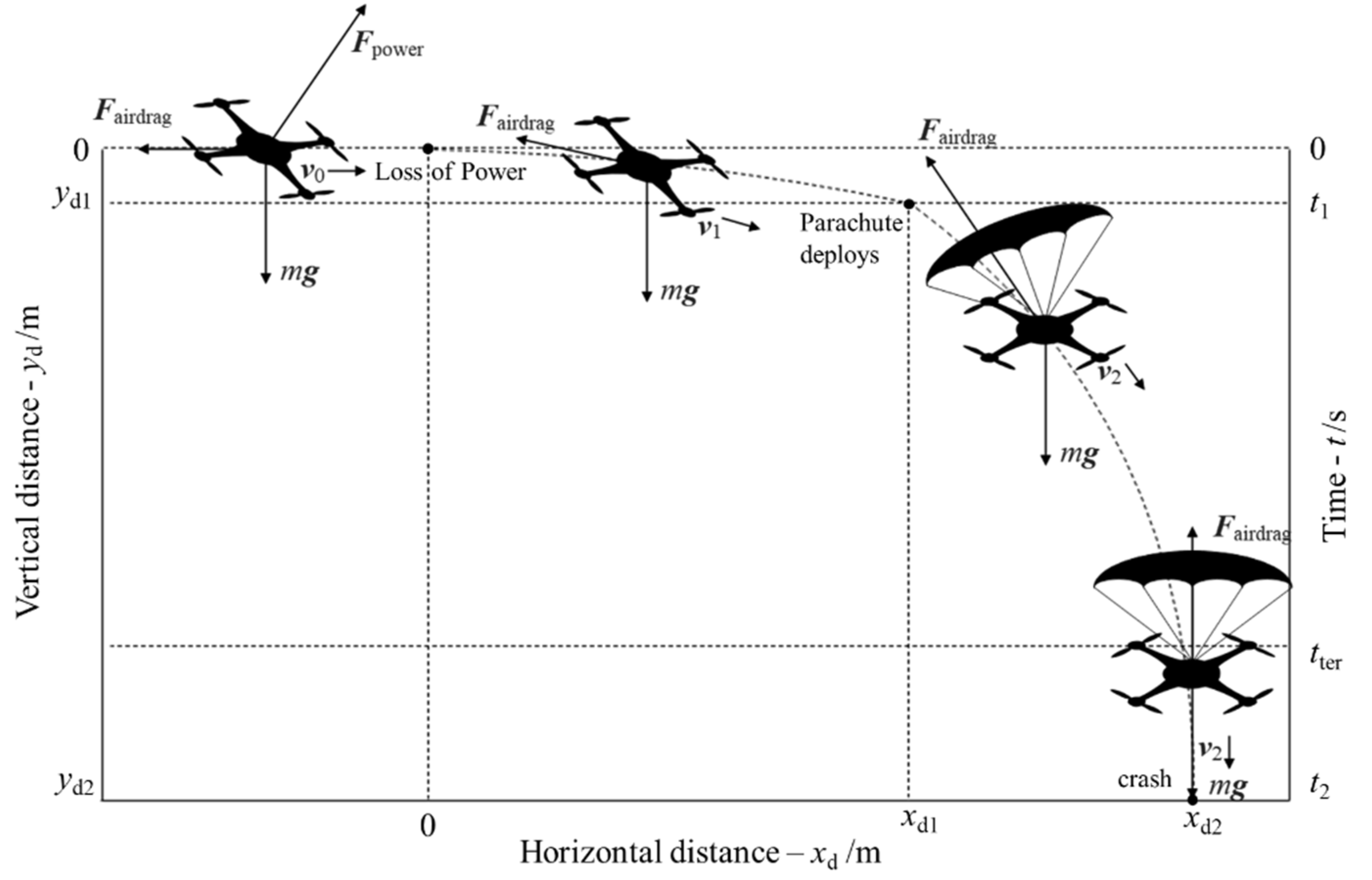
3.2.2. Parachute Systems

The purpose of the M2 measure in SORA is to reduce the impact of UAVs crashing on the ground. A widely discussed approach is the installation of a parachute system on UAVs because the deployment of parachutes induces a change in both the velocity and position of the UAV upon impact with the ground.

This subsection presents a derivation of the positional and velocity changes in the UAV considering the influence of the parachute system. Figure 6 illustrates the falling process of a quadrotor vehicle equipped with a parachute after experiencing a failure in the air. Under ideal conditions, the falling process is determined by gravity $m\mathit{g}$ and air drag ${\mathit{F}}_{\mathrm{airdrag}}$. The whole process can be divided into two stages. In the first stage, the UAV loses its power, and the status is transformed from a steady horizontal flight to a ballistic descent. In the second stage, the parachute system is activated, and the UAV enters a parachute descent phase. In the figure, $\mathit{v}$ represents the velocity direction, which is opposite to the direction of air resistance. $t_1$ denotes the parachute activation time, and $t_2$ represents the time of the UAV’s impact on the ground.

The air resistance acting on the UAV which is generated by a parachute system can be decomposed into a horizontal and a vertical component, which is given in Equation (14),

$$\left\{\begin{array}{c}{\mathit{F}}_{\mathrm{airdrag}}^x={\displaystyle \frac{1}{2}}\rho C_{\mathrm{drag}}{S}_{\mathrm{air}}{({\mathit{v}}^x)}^2,\\ {\mathit{F}}_{\mathrm{airdrag}}^y={\displaystyle \frac{1}{2}}\rho C_{\mathrm{drag}}{S}_{\mathrm{air}}{({\mathit{v}}^y)}^2.\end{array}\right.$$

(14)

where ${\mathit{F}}_{\mathrm{airdrag}}^x$ and ${\mathit{F}}_{\mathrm{airdrag}}^y$ represent the air resistance in the horizontal and vertical directions, respectively. $\rho$ denotes the air density, $S_{\mathrm{air}}$ is the effective front area, and $C_{\mathrm{drag}}$ is the air drag coefficient, which is a physical constant that depends only on the shape of an object. ${\mathit{v}}^x$ and ${\mathit{v}}^y$ are the horizontal and vertical velocities of the UAV. In the first stage, where $t\in [0,t_1]$, the initial velocity of the UAV is ${\mathit{v}}_o$, and the corresponding equations of motion can be derived as follows:

$$\begin{array}{c}m{\displaystyle \frac{d{v}^x}{dt}}=-{\displaystyle \frac{1}{2}}\rho C_{\mathrm{d},\mathrm{u}}{S}_{\mathrm{u}}{({\mathit{v}}^x)}^2,\\ m{\displaystyle \frac{d{\mathit{v}}^y}{dt}}=m\mathit{g}-{\displaystyle \frac{1}{2}}\rho C_{\mathrm{d},\mathrm{u}}{S}_{\mathrm{u}}{({\mathit{v}}^y)}^2.\end{array}$$

(15)

where $C_{\mathrm{d},\mathrm{u}}$ represents the air drag coefficient of the UAV and $S_{\mathrm{u}}$ denotes the effective front area of the UAV. The expression for the horizontal velocity ${\mathit{v}}_1^x(t)$ of the UAV during the first stage can be obtained with Equation (16) by solving the differential equation,

$${\mathit{v}}_1^x(t)={\displaystyle \frac{2m{\mathit{v}}_o}{\rho C_{\mathrm{d},\mathrm{u}}{S}_{\mathrm{u}}{\mathit{v}}_{0}t+2m}}.$$

(16)

Here, the vertical velocity ${\mathit{v}}_1^y(t)$ during the first stage is a piecewise function, as shown in Equation (17). Since the UAV undergoes accelerated motion in the vertical direction with an initial velocity of 0, i.e., ${\mathit{v}}_1^y\in (0,{\mathit{v}}_{\mathrm{b}}^{\mathrm{ter}})$, the expression for ${\mathit{v}}_1^y(t)$ can be derived. ${\mathit{v}}_{\mathrm{b}}^{\mathrm{ter}}$ represents the terminal velocity of the UAV in ballistic descent mode.

$$t=\left\{\begin{array}{ll}\sqrt{{\displaystyle \frac{2m}{\mathit{g}\rho C_{\mathrm{d},\mathrm{u}}{S}_{\mathrm{u}}}}}\mathrm{arctanh}(\sqrt{{\displaystyle \frac{\rho C_{\mathrm{d},\mathrm{u}}{S}_{\mathrm{u}}}{2m\mathit{g}}}}{\mathit{v}}_1^y)\hfill & {\mathit{v}}_1^y\in (0,{\mathit{v}}_{\mathrm{b}}^{\mathrm{ter}}),\hfill \\ \sqrt{{\displaystyle \frac{2m}{\mathit{g}\rho C_{\mathrm{d},\mathrm{u}}{S}_{\mathrm{u}}}}}\mathrm{arccoth}(\sqrt{{\displaystyle \frac{\rho C_{\mathrm{d},\mathrm{u}}{S}_{\mathrm{u}}}{2m\mathit{g}}}}{\mathit{v}}_1^y)\hfill & {\mathit{v}}_1^y\in ({\mathit{v}}_{\mathrm{b}}^{\mathrm{ter}},+\infty ).\hfill \end{array}\right.$$

(17)

$${\mathit{v}}_1^y(t)=\sqrt{{\displaystyle \frac{2m\mathit{g}}{\rho C_{\mathrm{d},\mathrm{u}}{S}_{\mathrm{u}}}}}\tanh \left(\sqrt{{\displaystyle \frac{\mathit{g}\rho C_{\mathrm{d},\mathrm{u}}{S}_{\mathrm{u}}}{2m}}}t\right),$$

(18)

At time $t_1$, the parachute fully deploys, and the motion of the UAV transitions into the second stage, the parachute descent phase. In this phase, $t\in (t_1,t_2]$, the UAV and parachute system are treated as a single ideal motion model. Following a similar approach as the previous motion analysis, the equations of the second phase can be derived in Equation (19)

$$\begin{array}{l}{\mathit{v}}_2^x(t)={\displaystyle \frac{2m{\mathit{v}}_1^x(t_1)}{\rho C_{\mathrm{d},\mathrm{p}}{S}_{\mathrm{p}}{\mathit{v}}_1^x(t_1)t+2m}},\\ {\mathit{v}}_2^y(t)=\sqrt{{\displaystyle \frac{2m\mathit{g}}{\rho C_{\mathrm{d},\mathrm{p}}{S}_{\mathrm{p}}}}}\tanh \left(\sqrt{{\displaystyle \frac{\mathit{g}\rho C_{\mathrm{d},\mathrm{p}}{S}_{\mathrm{p}}}{2m}}}t+\mathrm{arctanh}\left(\sqrt{{\displaystyle \frac{\rho C_{\mathrm{d},\mathrm{p}}{S}_{\mathrm{p}}}{2m\mathit{g}}}}{\mathit{v}}_1^y(t_1)\right)\right),\end{array}$$

(19)

where ${\mathit{v}}_2^x(t)$ and ${\mathit{v}}_2^y(t)$ represent the horizontal and vertical velocities of the UAV in the second stage. ${\mathit{v}}_1^x(t_1)$ and ${\mathit{v}}_1^y(t_1)$ are the instantaneous horizontal and vertical velocities of the UAV at time $t_1$, respectively. $C_{\mathrm{d},\mathrm{p}}$ denotes the air drag coefficient of the entire parachute system, and $S_{\mathrm{p}}$ represents the effective front area of the parachute system. By integrating the velocities of the UAV in both stages and summing the results, the equations for the horizontal displacement ${\mathit{x}}_{\mathrm{d}}$ and vertical displacement ${\mathit{y}}_{\mathrm{d}}$ to the ground impact point can be obtained,

$$\begin{array}{ll}{\mathit{x}}_{\mathrm{d}}& ={\displaystyle {\int }_0^{t_1}{\mathit{v}}_1^x}(t)dt+{\displaystyle {\int }_{t_1}^{t_2}{\mathit{v}}_2^x}(t)dt\\ & ={\displaystyle \frac{2m}{\rho C_{\mathrm{d},\mathrm{u}}{S}_{\mathrm{u}}}}\ln \left({\displaystyle \frac{\rho C_{\mathrm{d},\mathrm{u}}{S}_{\mathrm{u}}{\mathit{v}}_0{t}_1+2m}{2m}}\right)+{\displaystyle \frac{2m}{\rho C_{\mathrm{d},\mathrm{p}}{S}_{\mathrm{p}}}}\ln \left({\displaystyle \frac{\rho C_{\mathrm{d},\mathrm{p}}{S}_{\mathrm{p}}{\mathit{v}}_1^x(t_1)t_2+2m}{\rho C_{\mathrm{d},\mathrm{p}}{S}_{\mathrm{p}}{\mathit{v}}_1^x(t_1)t_1+2m}}\right),\\ {\mathit{y}}_{\mathrm{d}}& ={\displaystyle {\int }_0^{t_1}{\mathit{v}}_1^y}(t)dt+{\displaystyle {\int }_{t_1}^{t_2}{\mathit{v}}_2^y}(t)dt\\ & ={\displaystyle \frac{2m}{\rho C_{\mathrm{d},\mathrm{u}}{S}_{\mathrm{u}}}}\ln \left(\cosh \left(\sqrt{{\displaystyle \frac{\mathit{g}\rho C_{\mathrm{d},\mathrm{u}}{S}_{\mathrm{u}}}{2m}}}{t}_1\right)\right)+\\ & {\displaystyle \frac{2m}{\rho C_{\mathrm{d},\mathrm{p}}{S}_{\mathrm{p}}}}\ln \left({\displaystyle \frac{\cosh \left(\sqrt{\frac{\mathit{g}\rho C_{\mathrm{d},\mathrm{p}}{S}_{\mathrm{p}}}{2m}}{t}_2+\mathrm{arctanh}\left(\sqrt{\frac{\rho C_{\mathrm{d},\mathrm{p}}{S}_{\mathrm{p}}}{2m\mathit{g}}}{\mathit{v}}_1^y(t_1)\right)\right)}{\cosh \left(\sqrt{\frac{\mathit{g}\rho C_{\mathrm{d},\mathrm{p}}{S}_{\mathrm{p}}}{2m}}{t}_1+\mathrm{arctanh}\left(\sqrt{\frac{\rho C_{\mathrm{d},\mathrm{p}}{S}_{\mathrm{p}}}{2m\mathit{g}}}{\mathit{v}}_1^y(t_1)\right)\right)}}\right).\end{array}$$

(20)

The purpose of calculating the horizontal displacement ${\mathit{x}}_{\mathrm{d}}$ is to accurately represent the change in coordinates between the point of impact and failure location of the UAV, while computing the vertical displacement ${\mathit{y}}_{\mathrm{d}}$ serves to estimate its total descent duration. The final phase of its motion before impact can be approximated as linear motion when the UAV descends under the parachute descent model. The distance $d_{\mathrm{p}}$ of the ground casualty area $A_{\mathrm{c},\mathrm{p}}$ can be calculated based on the value of the velocity ${\mathit{v}}_{\mathrm{c},\mathrm{p}}$ at the moment of impact. Assuming the UAV’s flight altitude is $h_{\mathrm{u}}=\left|{\mathit{y}}_{\mathrm{d}}\right|$, the time $t_2$ can be calculated accordingly. ${\mathit{v}}_{\mathrm{c},\mathrm{p}}^x={\mathit{v}}_2^x(t_2)$ and ${\mathit{v}}_{\mathrm{c},\mathrm{p}}^y={\mathit{v}}_2^y(t_2)$ represent the horizontal and vertical velocity of the UAV at the moment of impact in the parachute descent model, and thus Equation (21) is derived,

$$d_{\mathrm{p}}=h_{\mathrm{p}}{\displaystyle \frac{\left|{\mathit{v}}_{\mathrm{c},\mathrm{p}}^x\right|}{\left|{\mathit{v}}_{\mathrm{c},\mathrm{p}}^y\right|}}.$$

(21)

Additionally, a special case needs to be considered. According to Equation (19), if the descent time is sufficiently long, i.e., $t\to +\infty$, then ${\mathit{v}}_2^x(t)\to 0$, and ${\mathit{v}}_2^y(t)\to {\mathit{v}}_{\mathrm{p}}^{\mathrm{ter}}$. At this point, the parachute descent model reaches a steady state, and gravity equals air resistance. In the ideal model, when the UAV reaches terminal velocity ${\mathit{v}}_{\mathrm{p}}^{\mathrm{ter}}$, it can be assumed that $d_{\mathrm{p}}=0$.

$$\begin{array}{l}0=m\mathit{g}-{\displaystyle \frac{1}{2}}\rho C_{\mathrm{d},\mathrm{p}}{S}_{\mathrm{p}}{({\mathit{v}}_{\mathrm{p}}^{\mathrm{ter}})}^2,\\ {\mathit{v}}_{\mathrm{p}}^{\mathrm{ter}}=\sqrt{{\displaystyle \frac{2m\mathit{g}}{\rho C_{\mathrm{d},\mathrm{p}}{S}_{\mathrm{p}}}}}.\end{array}$$

(22)

Fixed-wing UAVs have a more complex fall process when they lose power due to their different propulsion model compared to multirotor UAVs. However, this paper does not consider the complex effects brought by aerodynamics. Under ideal conditions, the fixed-wing UAV fall process is still divided into two stages. Figure 7 illustrates the falling process of a fixed-wing vehicle equipped with a parachute after experiencing a failure in the air.

In the first stage, after a power failure, the fixed-wing UAV is set to execute a gliding flight maneuver. In the horizontal direction, the motion analysis is similar to that of a multirotor UAV. The horizontal velocity ${\mathit{v}}_1^{\mathrm{f},x}(t)$ of the fixed-wing UAV in the first stage is denoted as

$${\mathit{v}}_1^{\mathrm{f},x}(t)={\displaystyle \frac{2m{\mathit{v}}_o}{\rho C_{\mathrm{d},\mathrm{u}}{S}_{\mathrm{u}}{\mathit{v}}_{0}t+2m}}.$$

(23)

In the vertical direction, during the brief period between the power failure and the deployment of the parachute system, assuming the aircraft’s attitude remains stable, it is primarily influenced by the lift generated by the wings. The augmentation of air resistance is minimal and can be considered negligible. The motion process can be expressed as Equation (24),

$$m{\displaystyle \frac{d{\mathit{v}}_1^{\mathrm{f},y}}{dt}}=m\mathit{g}-{\mathit{F}}_{\mathrm{lift}}.$$

(24)

where ${\mathit{F}}_{\mathrm{lift}}$ represents the lift force acting on the fixed-wing UAV, which can be calculated as Equation (25),

$${\mathit{F}}_{\mathrm{lift}}={\displaystyle \frac{1}{2}}\rho {({\mathit{v}}_1^{\mathrm{f},x})}^2{C}_{\mathrm{L}}{S}_{\mathrm{W}},$$

(25)

where $C_{\mathrm{L}}$ represents the lift coefficient under the UAV’s current flight conditions, and $S_{\mathrm{W}}$ denotes the wing area. These two parameters can be obtained by analyzing the motion state of the UAV under steady conditions, with no acceleration,

$$\begin{array}{l}0=m\mathit{g}-{\displaystyle \frac{1}{2}}\rho {\mathit{v}}_0^2{C}_{\mathrm{L}}{S}_{\mathrm{W}},\\ C_{\mathrm{L}}{S}_{\mathrm{W}}=\left|{\displaystyle \frac{2m\mathit{g}}{\rho {\mathit{v}}_0^2}}\right|.\end{array}$$

(26)

${\mathit{v}}_1^{\mathrm{f},y}(t)$ represents the vertical velocity of the fixed-wing UAV during the first stage. Equation (27) can be derived by solving the differential equation,

$${\mathit{v}}_1^{\mathrm{f},y}(t)=\mathit{g}t+{\displaystyle \frac{4m^2\mathit{g}}{\rho C_{\mathrm{d},\mathrm{u}}{S}_{\mathrm{u}}{\mathit{v}}_0(\rho C_{\mathrm{d},\mathrm{u}}{S}_{\mathrm{u}}{\mathit{v}}_{0}t+2m)}}-{\displaystyle \frac{2m\mathit{g}}{\rho C_{\mathrm{d},\mathrm{u}}{S}_{\mathrm{u}}{\mathit{v}}_0}}.$$

(27)

In the second stage, the parachute system fully deploys. After a brief period of overload, the fixed-wing UAV loses most of its horizontal velocity and the lift generated by its wings. At this stage, it is primarily influenced by gravity and air resistance, and the effect of lift in the vertical direction can be neglected. The motion analysis of the fixed-wing UAV is similar to that of the multirotor UAV, so the detailed derivation will not be repeated here.

The motion process expressions for the second stage are given as ${\mathit{v}}_2^{\mathrm{f},x}(t)$ and ${\mathit{v}}_2^{\mathrm{f},y}(t)$, and the displacement expressions relative to the ground impact point for both stages are ${\mathit{x}}_{\mathrm{d}}^{\mathrm{f}}$ and ${\mathit{y}}_{\mathrm{d}}^{\mathrm{f}}$,

$$\begin{array}{l}{\mathit{v}}_2^{\mathrm{f},x}(t)={\displaystyle \frac{2m{\mathit{v}}_1^{\mathrm{f},x}(t_1)}{\rho C_{\mathrm{d},\mathrm{p}}{S}_{\mathrm{p}}{\mathit{v}}_1^{\mathrm{f},x}(t_1)t+2m}},\\ {\mathit{v}}_2^{\mathrm{f},y}(t)=\sqrt{{\displaystyle \frac{2m\mathit{g}}{\rho C_{\mathrm{d},\mathrm{p}}{S}_{\mathrm{p}}}}}\tanh \left(\sqrt{{\displaystyle \frac{\mathit{g}\rho C_{\mathrm{d},\mathrm{p}}{S}_{\mathrm{p}}}{2m}}}t+\mathrm{arctanh}\left(\sqrt{{\displaystyle \frac{\rho C_{\mathrm{d},\mathrm{p}}{S}_{\mathrm{p}}}{2m\mathit{g}}}}{\mathit{v}}_1^{\mathrm{f},y}(t_1)\right)\right),\end{array}$$

(28)

$$\begin{array}{l}{\mathit{x}}_{\mathrm{d}}^{\mathrm{f}}={\displaystyle \frac{2m}{\rho C_{\mathrm{d},\mathrm{u}}{S}_{\mathrm{u}}}}\ln ({\displaystyle \frac{\rho C_{\mathrm{d},\mathrm{u}}{S}_{\mathrm{u}}{\mathit{v}}_0{t}_1+2m}{2m}})+{\displaystyle \frac{2m}{\rho C_{\mathrm{d},\mathrm{p}}{S}_{\mathrm{p}}}}\ln ({\displaystyle \frac{\rho C_{\mathrm{d},\mathrm{p}}{S}_{\mathrm{p}}{\mathit{v}}_1^{\mathrm{f},x}(t_1)t_2+2m}{\rho C_{\mathrm{d},\mathrm{p}}{S}_{\mathrm{p}}{\mathit{v}}_1^{\mathrm{f},x}(t_1)t_1+2m}}),\\ \begin{array}{c}{\mathit{y}}_{\mathrm{d}}^{\mathrm{f}}={\displaystyle \frac{1}{2}}\mathit{g}{t}_1^2+{\displaystyle \frac{4m^2\mathit{g}}{(\rho C_{\mathrm{d},\mathrm{u}}{S}_{\mathrm{u}}{\mathit{v}}_0{)}^2}}\ln \left({\displaystyle \frac{\rho C_{\mathrm{d},\mathrm{u}}{S}_{\mathrm{u}}{\mathit{v}}_0{t}_1+2m}{2m}}\right)-{\displaystyle \frac{2m\mathit{g}}{\rho C_{\mathrm{d},\mathrm{u}}{S}_{\mathrm{u}}{\mathit{v}}_0}}{t}_1+\\ {\displaystyle \frac{2m}{\rho C_{\mathrm{d},\mathrm{p}}{S}_{\mathrm{p}}}}\ln \left({\displaystyle \frac{\cosh \left(\sqrt{\frac{\mathit{g}\rho C_{\mathrm{d},\mathrm{p}}{S}_{\mathrm{p}}}{2m}}{t}_2+\mathrm{arctanh}\left(\sqrt{\frac{\rho C_{\mathrm{d},\mathrm{p}}{S}_{\mathrm{p}}}{2m\mathit{g}}}{\mathit{v}}_1^{\mathrm{f},y}(t_1)\right)\right)}{\cosh \left(\sqrt{\frac{\mathit{g}\rho C_{\mathrm{d},\mathrm{p}}{S}_{\mathrm{p}}}{2m}}{t}_1+\mathrm{arctanh}\left(\sqrt{\frac{\rho C_{\mathrm{d},\mathrm{p}}{S}_{\mathrm{p}}}{2m\mathit{g}}}{\mathit{v}}_1^{\mathrm{f},y}(t_1)\right)\right)}}\right).\end{array}\end{array}$$

(29)

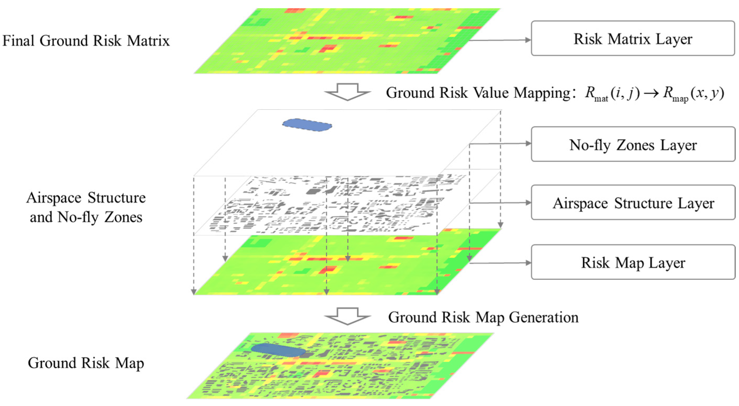
4. Generation of Ground Risk Map

4.1. Final UAV Ground Risk Matrix

The ground risk grid in this paper differs from the previous studies [9,19,34] which primarily focused on risk analysis based on flight paths or missions. Instead, it adopts a matrix format, allowing for the modular addition or removal of risk assessment components. This approach enables a broader analysis of UAV’s operation risk in urban environments from a wide-area perspective.

According to Section 3.1, the expression for the expected casualties $E_{\mathrm{C},\mathrm{p}}$ in the parachute descent model can be constructed as Equation (30),

$$\begin{array}{l}{E}_{\mathrm{C},\mathrm{p}}=D_{\mathrm{p}}\cdot A_{\mathrm{c},\mathrm{p}}\cdot P_{\mathrm{f},\mathrm{p}},\\ E_{\mathrm{C},\mathrm{p}}=D_{\mathrm{p}}\cdot A_{\mathrm{c},\mathrm{b}}\cdot {\displaystyle \frac{1}{A_{\mathrm{c},\mathrm{b}}}}\cdot A_{\mathrm{c},\mathrm{p}}\cdot P_{\mathrm{f},\mathrm{p}}\cdot {\displaystyle \frac{1}{P_{\mathrm{f},\mathrm{b}}}}\cdot P_{\mathrm{f},\mathrm{b}}.\end{array}$$

(30)

The parachute system reduces the impact kinetic energy by decreasing the UAV’s impact velocity, which also reduces the casualty area on the ground. Therefore, $A_{\mathrm{c},\mathrm{b}}$ and $A_{\mathrm{c},\mathrm{p}}$ represent the casualty areas in the ballistic descent and parachute descent, respectively. Similarly, $P_{\mathrm{f},\mathrm{b}}$ and $P_{\mathrm{f},\mathrm{p}}$ denote the fatality rates in both models. For any risk unit $(i,j)$, the following can be defined:

$$\begin{array}{l}{M}_{\mathrm{p}}(i,j)={\displaystyle \frac{1}{A_{\mathrm{c},\mathrm{b}}}}\cdot A_{\mathrm{c},\mathrm{p}}\cdot P_{\mathrm{f},\mathrm{p}}\cdot {\displaystyle \frac{1}{P_{\mathrm{f},\mathrm{b}}}},\\ M_{\mathrm{s}}(i,j)=P_{\mathrm{f},\mathrm{b}}.\end{array}$$

(31)

Taking a multirotor UAV as an example, $E_{\mathrm{crash},\mathrm{p}}$ and $E_{\mathrm{crash},\mathrm{b}}$ represent the impact kinetic energy of the UAV in the parachute descent model and ballistic descent model, respectively, with $E_{\mathrm{crash},\mathrm{b}}>E_{\mathrm{crash},\mathrm{p}}$. The relationships between $E_{\mathrm{crash},\mathrm{p}}$, $E_{\mathrm{crash},\mathrm{b}}$, and $\beta$ are discussed as follows:

• When $E_{\mathrm{crash},\mathrm{b}}\le \beta$, i.e., $M_{\mathrm{s}}(i,j)=0$, and according to Equation (10), the intrinsic ground risk $R_{\mathrm{i}}(i,j)=0$.
• When $E_{\mathrm{crash},\mathrm{b}}>\beta \ge E_{\mathrm{crash},\mathrm{p}}$, i.e., $M_{\mathrm{p}}(i,j)=0$, meaning the expected casualties of the parachute descent $E_{\mathrm{C},\mathrm{p}}=0$.
• When $E_{crash,p}\ge \beta$, Equation (32) can be defined,

  $$M_{\mathrm{p}}(i,j)={\displaystyle \frac{2h_{\mathrm{p}}\frac{\left|{\mathit{v}}_{\mathrm{c},\mathrm{b}}^x\right|}{\left|{\mathit{v}}_{\mathrm{c},\mathrm{b}}^y\right|}+\pi (r_{\mathrm{p}}+r_{\mathrm{u}})}{2h_{\mathrm{p}}\frac{\left|{\mathit{v}}_{\mathrm{c},\mathrm{p}}^x\right|}{\left|{\mathit{v}}_{\mathrm{c},\mathrm{p}}^y\right|}+\pi (r_{\mathrm{p}}+r_u)}}\cdot {\displaystyle \frac{[1-{(\frac{\beta }{E_{\mathrm{crash},\mathrm{p}}})}^{\frac{3}{P_{\mathrm{s}}}}][1-2{(\frac{\beta }{E_{\mathrm{crash},\mathrm{b}}})}^{\frac{3}{P_{\mathrm{s}}}}+\sqrt{\frac{\alpha }{\beta }}{(\frac{\beta }{E_{\mathrm{crash},\mathrm{b}}})}^{\frac{3}{P_{\mathrm{s}}}}]}{[1-{(\frac{\beta }{E_{\mathrm{crash},\mathrm{b}}})}^{\frac{3}{P_{\mathrm{s}}}}][1-2{(\frac{\beta }{E_{\mathrm{crash},\mathrm{p}}})}^{\frac{3}{P_{\mathrm{s}}}}+\sqrt{\frac{\alpha }{\beta }}{(\frac{\beta }{E_{\mathrm{crash},\mathrm{p}}})}^{\frac{3}{P_{\mathrm{s}}}}]}}.$$

  (32)

The parachute system mitigates ground risk by reducing the UAV’s impact velocity. In Equation (32), the first term reflects how the parachute reduces the casualty area by lowering the velocity, while the second term represents how the parachute decreases the fatality rate by reducing the kinetic energy, which is itself a function of impact velocity. Based on Equation (10), the following can be derived:

$$E_{\mathrm{C},\mathrm{p}}=R_{\mathrm{i}}(i,j)\cdot M_{\mathrm{p}}(i,j)\cdot M_{\mathrm{s}}(i,j).$$

(33)

Equation (33) can be understood as the mitigation effect of risk reduction measures on the intrinsic ground risk of the UAV. Two matrices, denoted as ${\mathit{M}}_{\mathrm{s}}$ and ${\mathit{M}}_{\mathrm{p}}$, are established to quantify the respective impacts of ground sheltering (M1 measure) and UAV’s parachute system (M2 measure). By incorporating both ground sheltering and the parachute system, the intrinsic ground risk can be effectively mitigated. The construction of the ground risk mitigation matrix ${\mathit{M}}_{n\times m}$ is used to represent the impact of these two mitigations on reducing ground risk,

$$M(i,j)=\left\{\begin{array}{ll}\eta M_{\mathrm{p}}(i,j)\cdot M_{\mathrm{s}}(i,j)+(1-\eta )M_{\mathrm{s}}(i,j)\hfill & E_{\mathrm{crash},\mathrm{p}}\ge \beta ,\hfill \\ (1-\eta )M_{\mathrm{s}}(i,j)\hfill & E_{\mathrm{crash},\mathrm{b}}>\beta \ge E_{\mathrm{crash},\mathrm{p}},\hfill \\ 0\hfill & E_{\mathrm{crash},\mathrm{b}}\le \beta .\hfill \end{array}\right.$$

(34)

where element $M(i,j)$ of matrix ${\mathit{M}}_{n\times m}$ represents the value of ground risk reduction in cell $(i,j)$, and $\eta$ is the parachute deployment success rate, which is influenced by factors such as UAV model, deployment altitude, velocity, and parachute system sensors. A detailed discussion of these factors is beyond the scope of this paper.

The final ground risk value $R_{\mathrm{f}}(i,j)$ of a UAV can be derived by utilizing Equations (5), (30) and (31),

$$\begin{array}{ll}{R}_{\mathrm{f}}(i,j)& =D_{\mathrm{p}}(i,j)\cdot A_{\mathrm{c},\mathrm{b}}\cdot {\displaystyle \frac{1}{A_{\mathrm{c},\mathrm{b}}}}\cdot A_{\mathrm{c},\mathrm{p}}\cdot P_{\mathrm{f},\mathrm{p}}\cdot {\displaystyle \frac{1}{P_{\mathrm{f},\mathrm{b}}}}\cdot P_{\mathrm{f},\mathrm{b}}\\ & =D_{\mathrm{p}}(i,j)\cdot A_{\mathrm{c},\mathrm{b}}\cdot M_{\mathrm{p}}(i,j)\cdot M_{\mathrm{s}}(i,j)\\ & =R_{\mathrm{i}}(i,j)\cdot M_{\mathrm{p}}(i,j)\cdot M_{\mathrm{s}}(i,j).\end{array}$$

(35)

By discussing the success rate $\eta$ of the parachute system in (34), the final ground risk assessment can be derived as

$$\begin{array}{ll}{R}_{\mathrm{f}}(i,j)& =\left\{\begin{array}{ll}{R}_{\mathrm{i}}(i,j)\eta M_{\mathrm{p}}(i,j)\cdot M_{\mathrm{s}}(i,j)+(1-\eta )M_{\mathrm{s}}(i,j)\hfill & E_{\mathrm{crash},\mathrm{p}}\ge \beta \hfill \\ R_{\mathrm{i}}(i,j)(1-\eta )M_{\mathrm{s}}(i,j)\hfill & E_{\mathrm{crash},\mathrm{b}}>\beta \ge E_{\mathrm{crash},\mathrm{p}}\hfill \\ 0\hfill & E_{\mathrm{crash},\mathrm{b}}\le \beta \hfill \end{array}\right.\\ & =R_{\mathrm{i}}(i,j)\cdot M(i,j).\end{array}$$

(36)

As a result, the process of calculating the final ground risk matrix is depicted in Figure 8. The final ground risk matrix ${\mathit{R}}_{\mathrm{f}}$, after applying mitigation measures, is equal to the Hadamard product of the intrinsic ground risk matrix ${\mathit{R}}_{\mathrm{i}}$ and the ground risk mitigation matrix $\mathit{M}$.

$${\mathit{R}}_{\mathrm{f}}={\mathit{R}}_{\mathrm{i}}\odot \mathit{M}.$$

(37)

4.2. Ground Risk Map

The ground risk map is a grid-based map in which each cell is associated with a specific risk value. The ground risk map covers large predefined areas and takes into account UAV specifications, flight speed, and altitude, as well as the characteristics of the environment sheltering.

After calculating the final ground risk matrix, the corresponding UAV ground risk map for the geographic grid can be generated using the coordinate transformation method outlined in Section 3.1, i.e., $R_{\mathrm{map}}(x,y)=R_{\mathrm{f}}(i,j)$. The process of generating a ground risk map from the final ground risk matrix is illustrated in Figure 9. Firstly, the risk values in the final ground risk matrix are mapped onto the corresponding geographic grid $R_{\mathrm{map}}(x,y)$. Smoothing is applied to mitigate step changes at the edge of the grid to better approach the continuous change process of actual risk distribution. Subsequently, the airspace structure layer and no-fly zone layer are overlaid on the geographic grid to establish a comprehensive ground risk map. In the following section, a case study on the generation of risk maps is presented.

5. Experiments and Discussions

In this section, four sets of case study experiments were conducted. The ground risk for four different types of UAVs under six different scenarios is calculated. We provide an overview of the experimental parameter settings in Section 5.1 and subsequently present the simulation results, accompanied by data analysis, in Section 5.2. The empirical investigation aims to examine how UAV parameters, flight altitude, and parachute system success rate impact the final ground risk value.

5.1. Simulation Scenario and Parameter Settings

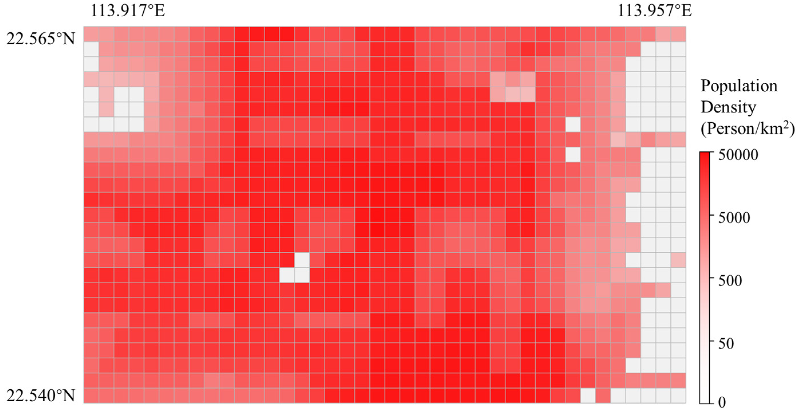
5.1.1. Simulation Scenario, Datasets, and Parameter Settings

To validate the proposed method and framework, a simulation was conducted on a real area with a size of 2.5 km × 4 km in Shenzhen, China. The studied area is located between latitudes 22°540′ N~22°565′ N and longitudes113°917′ E~113°957′ E. Shenzhen has a high average population density of 8889 people/km², and the environmental parameters used in the simulation are shown in

Table 2. Simulation and environmental parameters.

Parameters	Value
Gravitational acceleration $\mathit{g}$ (m/s2)	9.8
Air density $\rho$ (kg/m3)	1.225
Human average height $h_{\mathrm{p}}$ (m)	1.8
Human average radius $r_{\mathrm{p}}$ (m)	0.3
Operating altitude $h_{\mathrm{u}}$ (m)	30/60/90
$\alpha$ (J)	3.4 × 104
$\beta$ (J)	34
Parachute system success rate $\eta$	95%

.

The map data used in this paper are sourced from Google Maps [39] and Open Street Map (OSM) [40], which were obtained in July 2024. Based on the satellite and topographic maps, this area is rasterized to a geographic map with a resolution of 100 m × 100 m to collect and calculate urban environmental data. The sheltering parameters were then defined according to Section 3.2.1. The population distribution data used in this study are from the WorldPop population dataset [41], as shown in Figure 10, which was developed based on the 2020 census and estimation results. The dataset has a grid resolution of 100 m × 100 m. Using the 3D urban geographic data, the airspace structure map for the region was generated. According to the regulations, airspace below 120 m in China is designated as suitable for small UAVs. Therefore, airspace structures were generated for three altitude layers: 30 m, 60 m, and 90 m.

5.1.2. UAV Parameter Settings

In the simulation, two different types of UAVs were considered, which include fixed-wing UAVs and multirotor UAVs. Specifically, the models used in this paper are Parrot Disco, Talon, DJI Phantom4, and DJI M350. Among these, Parrot Disco and Talon represent two kinds of fixed-wing UAVs, while DJI Phantom4 and DJI M350 are two multirotor UAVs. The performance data are primarily sourced from the manufacturers’ official manuals [22]. A normal distribution $\mathrm{N}(\mu ,\sigma )$ is used to describe a certain number of parameters, where μ is the mean and σ is the standard deviation. The parachute data are based on the actual parachute products [42] with the parameters listed in

Table 3. Parameters of the UAVs used as examples.

	Parrot Disco	Talon	DJI Phantom4	DJI M350
Type	Fixed wing	Fixed wing	Quadrotor	Quadrotor
Mass $m$ (kg)	0.75	3.75	1.39	9.2
Radius $r_{\mathrm{u}}$ (m)	0.575	0.88	0.18	0.45
Cruising speed ${\mathit{v}}_0$ (m/s)	N(15, 2.5)	N(18, 2.5)	N(15, 0.2)	N(23, 0.2)
Front area $S_{\mathrm{u}}$ (m2)	0.07	0.1	0.02	0.046
Drag coefficient of UAVs $C_{\mathrm{d},\mathrm{u}}$	N(0.9, 0.2)	N(0.9, 0.2)	N(0.8, 0.2)	N(0.8, 0.2)
Parachute area $S_{\mathrm{p}}$ (m2)	0.5	1	1.1	7.3
Drag coefficient of parachute $C_{\mathrm{d},\mathrm{p}}$	N(1.3, 0.2)	N(1.3, 0.2)	N(1.1, 0.2)	N(1.1, 0.2)
Parachute deployment time $t_1$ (s)	1.2	1.2	0.7	0.7

.

5.2. Case Study and Analyses

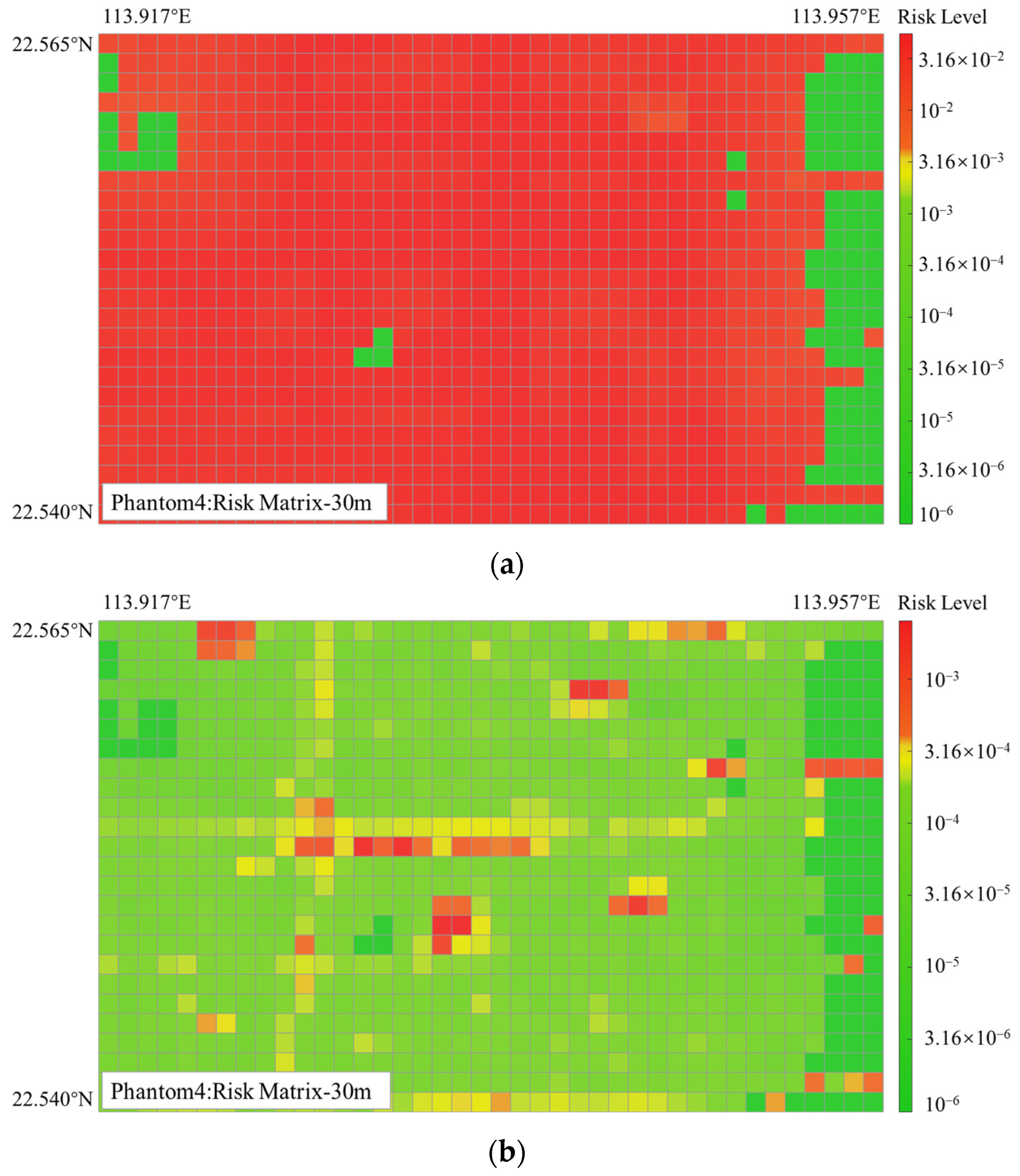
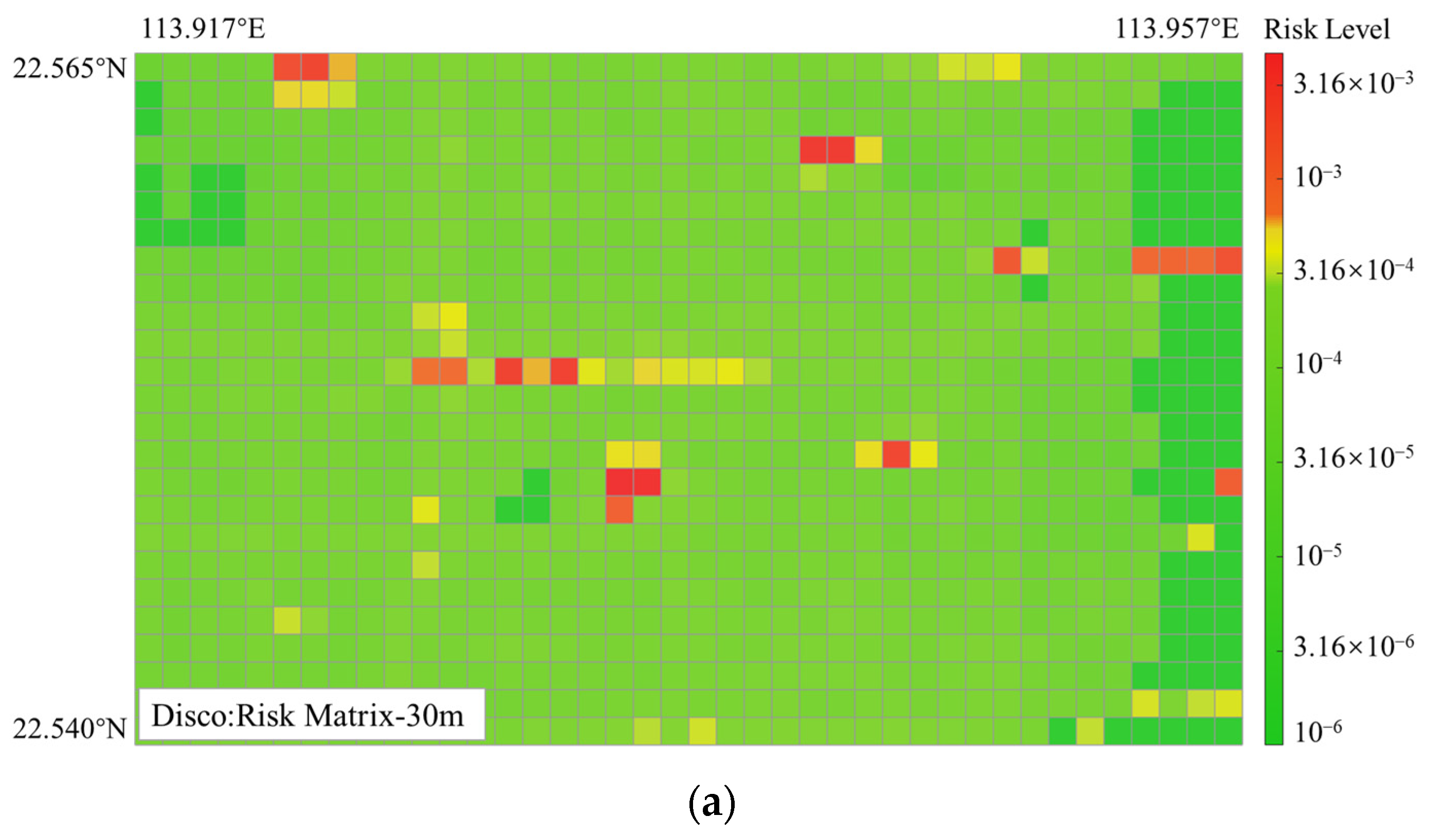
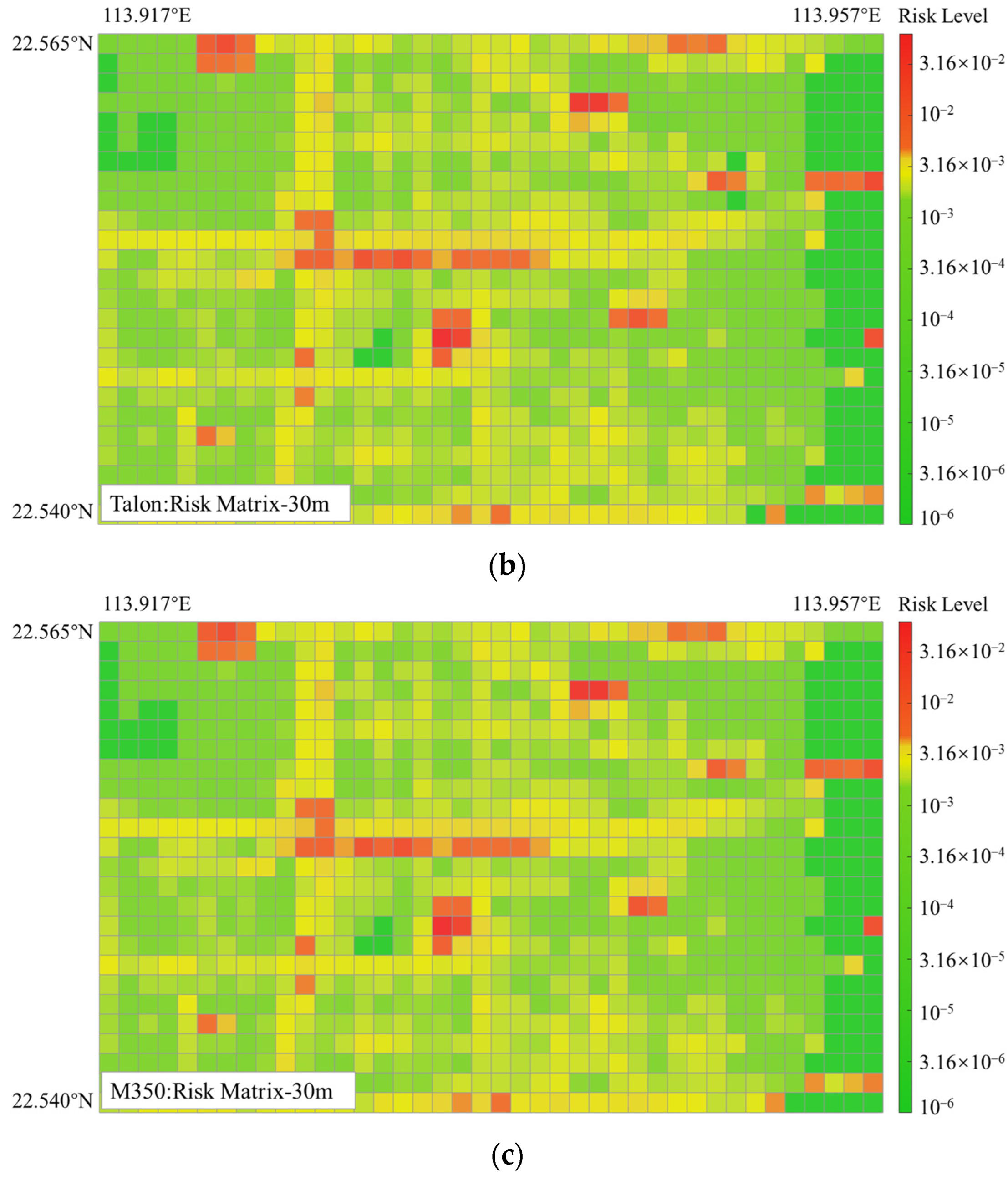
5.2.1. Results of Ground Risk Map Generation

In this subsection, the DJI Phantom4 quadrotor UAV is first considered. The intrinsic ground risk matrix is calculated and visualized, which is given in Figure 11a. Then, the risk mitigation matrix is computed at the operating altitude of 30 m, assuming a 95% parachute deployment success rate. The final ground risk matrix is determined, as shown in Figure 11b.

A general aviation airport in this vicinity has been designated as a no-fly zone in the case of low-altitude manned/unmanned aerial vehicle hybrid operation being unsatisfactory. A static ground risk map for DJI Phantom4 at a flight height of 30 m has been developed to comply with airspace structure restrictions in the area.

Additionally, interpolation and smoothing should be applied to the edge pixels of the visualized grid risk matrix to mitigate step changes in risk values. This process ensures that the risk map more accurately reflects real conditions. The final ground risk map is subsequently generated, as illustrated in Figure 12.

The grid risk matrix and risk map enable the quantification of the risk levels faced by urban populations in the event of a UAV crash over large city areas. The next subsections discuss the influence of other factors on ground risk under different scenarios.

Furthermore, this study presents the final ground risk matrices for three additional UAV types operating at a flight altitude of 30 m, with an assumed 95% success rate for parachute deployment, serving as a benchmark for comparative analysis, as shown in Figure 13.

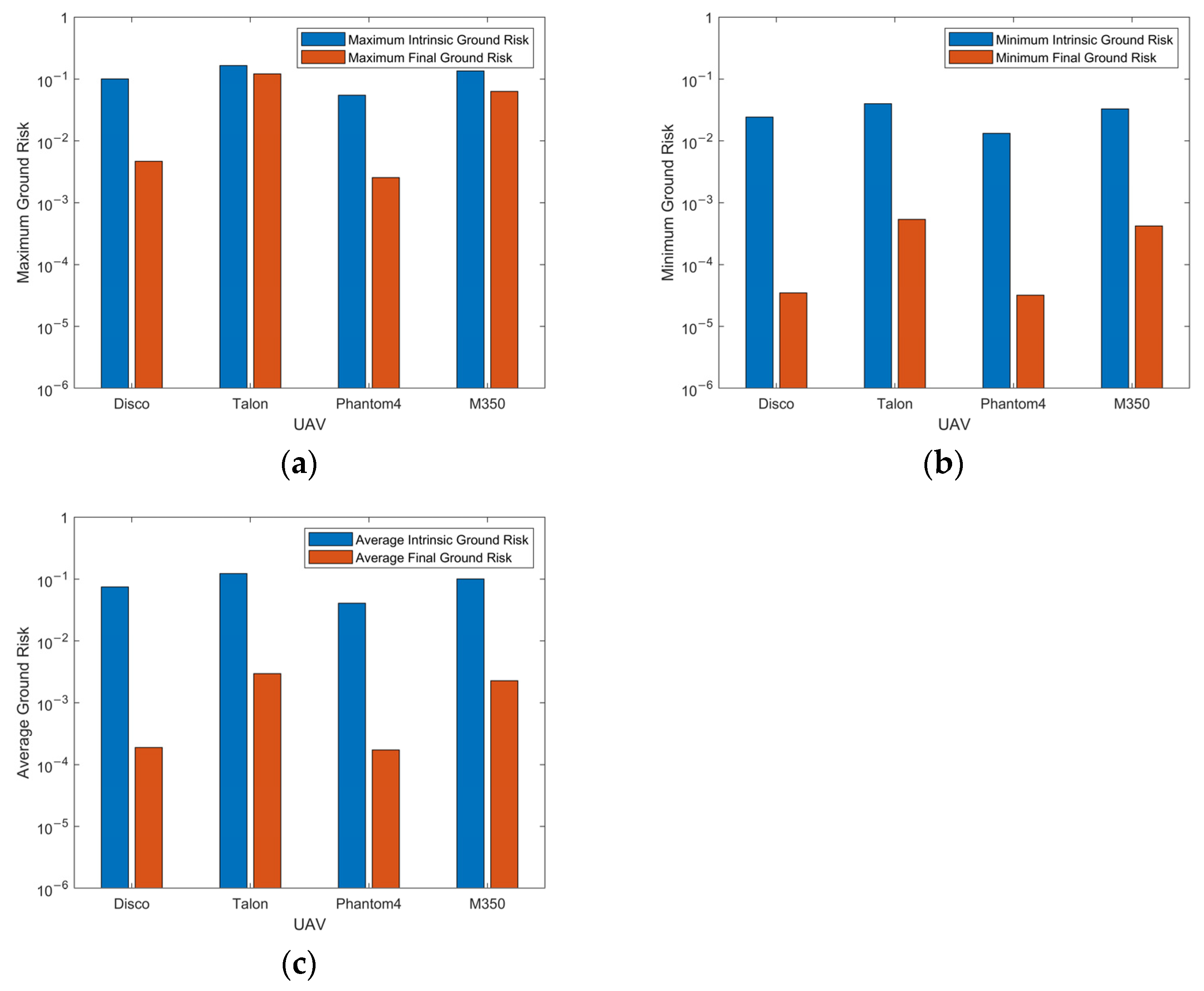
5.2.2. The Influence of UAV Parameters

Table 4. The final ground risk values (casualty/hour) of four types of UAVs.

UAV		30 m	60 m	90 m
Parrot Disco	Maximum	4.680 × 10−3	4.273 × 10−3	4.112 × 10−3
	Minimum	3.480 × 10−5	5.118 × 10−5	6.238 × 10−5
	Average	1.895 × 10−4	2.766 × 10−4	3.361 × 10−4
Talon	Maximum	1.213 × 10−1	1.290 × 10−1	1.319 × 10−1
	Minimum	5.395 × 10−4	6.094 × 10−4	6.518 × 10−4
	Average	2.957 × 10−3	3.331 × 10−3	3.553 × 10−3
DJI Phantom4	Maximum	2.549 × 10−3	2.130 × 10−3	1.956 × 10−3
	Minimum	3.198 × 10−5	3.301 × 10−5	3.343 × 10−5
	Average	1.727 × 10−4	1.778 × 10−4	1.798 × 10−4
DJI M350	Maximum	6.307 × 10−2	5.942 × 10−2	5.812 × 10−2
	Minimum	4.213 × 10−4	4.005 × 10−4	3.959 × 10−4
	Average	2.268 × 10−3	2.144 × 10−3	2.110 × 10−3

presents the final ground risk values (casualty/hour) for the four types of UAVs at a 95% parachute deployment success rate. To better reflect the impact of UAVs on populations, the maximum, minimum, and average risk levels are calculated only for grids with a population density greater than zero, excluding the cases where UAVs crash into uninhabited areas.

The analysis of the data reveals that the primary factors influencing the ground risk level are UAV characteristics, specifically mass and size. Larger UAVs tend to pose higher risk levels. In contrast, the flight altitude does not significantly affect the ground risk. For the Disco, Talon, and Phantom4 UAVs, there is a marginal increase in the maximum, minimum, and average risk values as flight altitudes rise, without any significant order-of-magnitude changes. The rationale behind this is that the impact kinetic energy resulting from a fall at a height of 30 m possesses sufficient potential to induce casualties upon contact with the ground. Therefore, the increase in flight altitude does not result in a corresponding elevation of the intrinsic ground risk.

The values of maximum risk, minimum risk, and average risk associated with M350 exhibit a notable degree of stability as the flight altitude increases. The stability of the M350 can be attributed to its utilization of a larger parachute system compared to the other UAVs. As flight altitude increases, the UAV’s final crashing velocity approaches the parachute system’s terminal velocity, thereby allowing the overall risk to remain relatively stable.

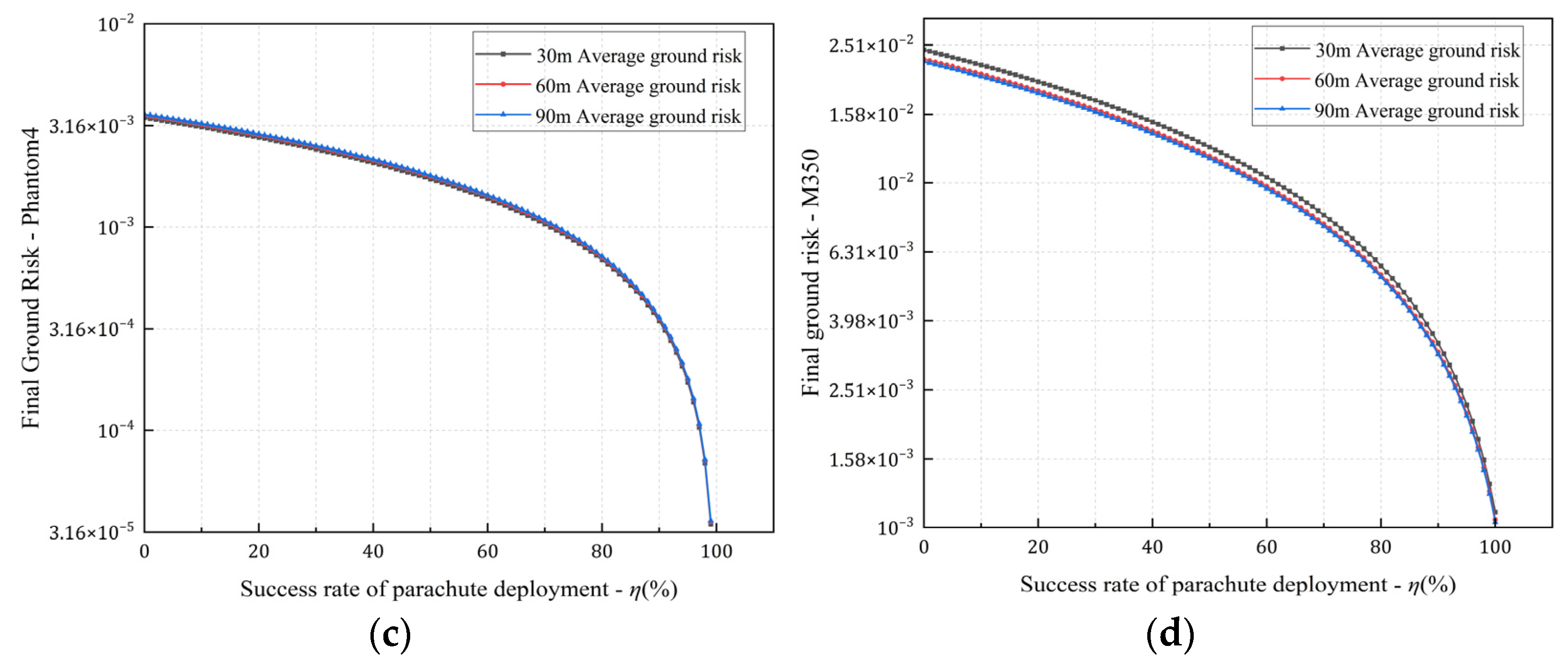
5.2.3. The Influence of UAV Flight Altitude on Risk Mitigations

This subsection examines the effectiveness of ground risk mitigation measures in reducing ground risk levels. The focus lies on assessing the risk mitigation level of the four UAVs at the flight altitudes of 30 and 90 m, as these altitudes represent the upper and lower boundaries within the simulation scenarios. The intrinsic ground risk is compared and the final ground risk for both altitudes is given. Detailed data are provided in

Table 5. The comparison of intrinsic risk values (casualty/hour) and final risk values for four UAVs.

UAV		30 m		90 m
		Intrinsic Risk	Final Risk	Intrinsic Risk	Final Risk
Parrot Disco	Maximum	1.008 × 10−1	4.680 × 10−3	8.861 × 10−2	4.112 × 10−3
	Minimum	2.438 × 10−2	3.480 × 10−5	2.214 × 10−2	6.238 × 10−5
	Average	7.485 × 10−2	1.895 × 10−4	6.577 × 10−2	3.361 × 10−4
Talon	Maximum	1.657 × 10−1	1.213 × 10−1	1.596 × 10−1	1.319 × 10−1
	Minimum	4.006 × 10−2	5.395 × 10−4	3.858 × 10−2	6.518 × 10−4
	Average	1.230 × 10−1	2.957 × 10−3	1.185 × 10−1	3.553 × 10−3
DJI Phantom4	Maximum	5.494 × 10−2	2.549 × 10−3	4.214 × 10−2	1.956 × 10−3
	Minimum	1.328 × 10−2	3.198 × 10−5	1.109 × 10−2	3.343 × 10−5
	Average	4.078 × 10−2	1.727 × 10−4	3.218 × 10−2	1.798 × 10−4
DJI M350	Maximum	1.359 × 10−1	6.307 × 10−2	1.023 × 10−1	5.812 × 10−2
	Minimum	3.286 × 10−2	4.213 × 10−4	2.473 × 10−2	3.959 × 10−4
	Average	1.009 × 10−1	2.268 × 10−3	7.593 × 10−2	2.110 × 10−3

.

As given in Table 5, at a flight altitude of 30 m, the average risk levels for the Disco, Talon, Phantom4, and M350 UAVs were mitigated by 2.532 × 10⁻², 2.404 × 10⁻², 4.234 × 10⁻², and 2.248 × 10⁻², respectively. The effectiveness of risk reduction is independent of the UAVs’ mass and size, which is primarily affected by the ground sheltering coefficient and the parachute system’s capabilities. In the selected urban environment, the average risk mitigation reached the 10⁻² level across the four UAVs, as illustrated in Figure 14. The maximum risk levels were mitigated by 4.643 × 10⁻², 7.320 × 10⁻¹, 4.639 × 10⁻², and 4.440 × 10⁻¹, while the minimum risk levels were reduced by 1.427 × 10⁻³, 1.347 × 10⁻², 2.997 × 10⁻³, and 1.282 × 10⁻². This suggests that the effectiveness of mitigation measures diminishes in high-density population areas, whereas it increases in low-density regions.

At a flight altitude of 90 m, the average risk levels for the Disco, Talon, Phantom4, and M350 UAVs were mitigated by 5.489 × 10⁻³, 2.998 × 10⁻², 5.748 × 10⁻³, and 2.779 × 10⁻², respectively. This indicates that the effectiveness of risk mitigation measures slightly increases with higher flight altitudes. The rationale is that as the flight height increases, the deployment time of the parachute system also extends, causing the impact velocity to approach terminal velocity. This is particularly evident in smaller UAVs, which maintain a mitigation capacity at the 10⁻² level, while some models can achieve the 10⁻³ level, as illustrated in Figure 15. Additionally, the mitigation capabilities for the maximum and minimum risk levels are comparable to those observed at a flight altitude of 30 m, showing no significant change.

The findings suggest that a well-designed parachute system can effectively mitigate risk values close to the 10⁻² level with a 95% success rate in deploying the parachute.

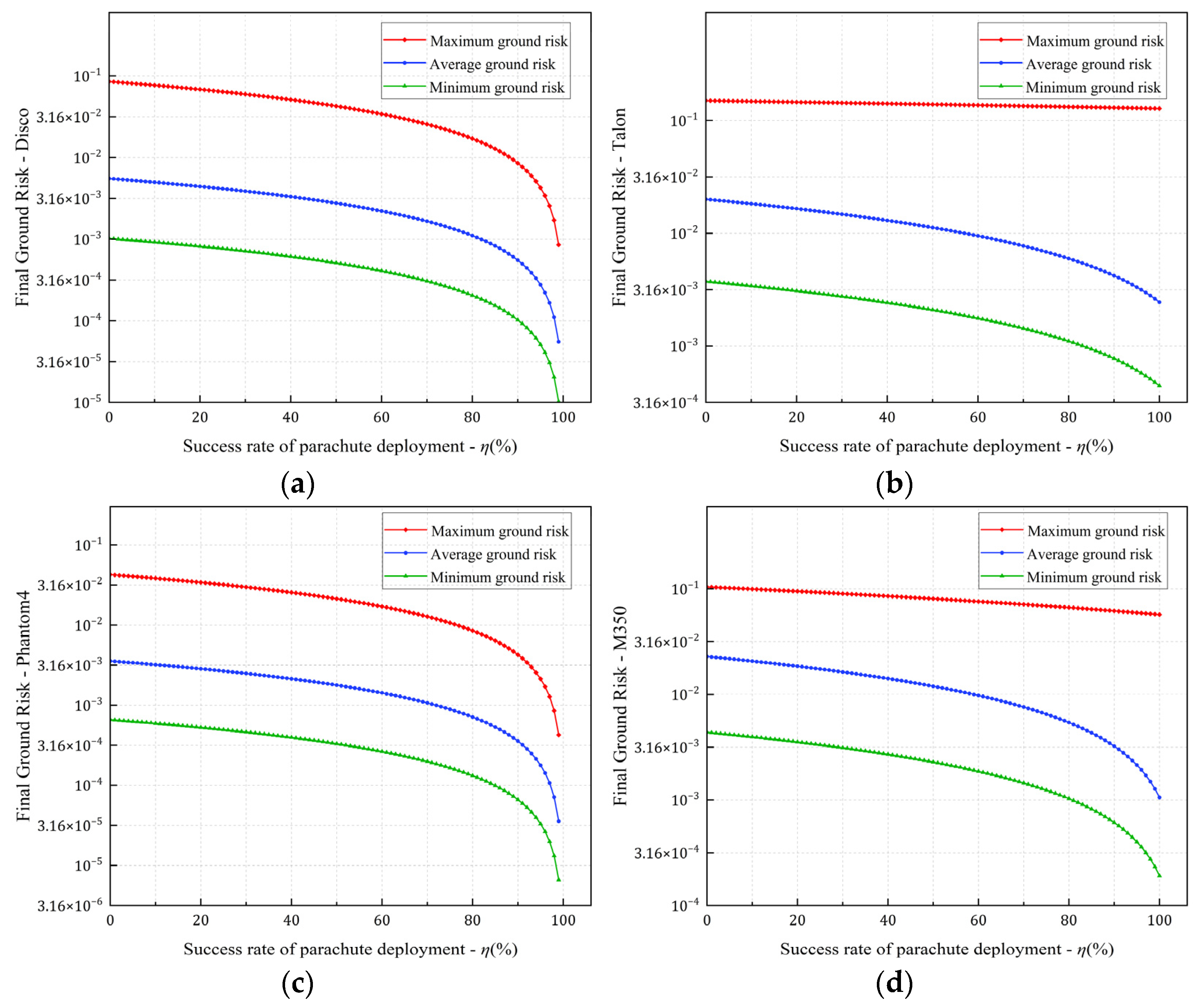
5.2.4. The Influence of Parachute Deployment Success Rate

Equation (34) establishes a linear model that incorporates the mitigation success rate η of a parachute system. Previous discussions have assumed a high success rate, implying that the parachute system can offer a relatively stable capacity for mitigation.

Therefore, this subsection examines the relationship between the risk values and the success rate of the parachute system, as illustrated in Figure 16. The findings indicate that the success rate of the UAV parachute system at a height of 30 m can serve as an indicative measure of its risk mitigation capability to a certain extent. The average risk values exhibit a significant reduction effect as the success rate increases.

The first set of analyses was conducted for the Disco and Phantom4, two smaller UAVs. The parachute system exhibits an average risk mitigation capability at the 10⁻¹ level when the success rate reaches 90%. Upon achieving a success rate of 100%, the parachute system demonstrates an average risk mitigation capability close to the 10⁻² level. For Talon and M350, two larger UAVs, the parachute system demonstrates an average risk mitigation capability close to the 10⁻¹ level with a 90% success rate, and the 10^−1.5 level with a 100% success rate.

This subsection also analyzes the relationship between the average risk values and the success rate at the altitudes of 30, 60, and 90 m, as shown in Figure 17. For Phantom 4 and M350, the two UAVs are equipped with larger parachute surface areas. The experimental findings suggest that flight altitude does not exert a significant influence on the average risk values; instead, the primary determinant remains the success rate of the parachute system. For Disco and Talon, which are equipped with smaller parachute surface areas, the average risk values exhibit a slight increase with altitude. However, the increase in values remains below the threshold of the 10^−0.5 level.

5.3. Discussion

The presented results show that a ground risk map generated by the proposed framework can quantify the risk to the population of a complex urban area. The proposed ground risk assessment framework is universally applicable and remains valid regardless of changes in urban scenes. The selection of Shenzhen as the simulation scenario is based on its status as a representative city with a well-established UAV industry. The framework can adapt the risk assessment module to meet local regulatory requirements, and it can be integrated into the Unmanned Aircraft System Traffic Management (UTM) system through the development of a 3D risk map layer using geographic information system (GIS) data, airspace databases, and weather forecasting. The ground risk map is able to detect the areas where the flight would be safe or not, as illustrated in the results in Section 5.2. It can be used to assess the risk of specific flight operations and grant permission to fly for the Equivalent Level of Safety (ELOS), which represents the safety standard for UAV operations. On the other hand, the proposed method can be used to define or modify the flight plan of UAVs operating in urban areas.

The ground risk map can be utilized by a risk-aware path planning algorithm to delineate low-risk paths in urban operations. The incorporation of a risk-aware path planner with the ground risk map offers an effective approach to significantly reduce risk with strategize missions, even within expansive urban areas. Several studies [24,30,31] have been conducted to address this issue. However, the risk maps utilized in these studies primarily focused on assessing the individual UAV mission rather than the impact of the ground. Consequently, these risk maps are inadequate for facilitating safe path planning when multiple UAVs are operating.

However, unlike the ground risk maps in research such as [22], the static ground risk map proposed in this paper only represents the location on the ground where the UAV crashes. The advantage of this lies in its ability to more effectively depict the collective impact of multiple UAVs within a given area. The derivation of the UAV failure location coordinates necessitates the consideration of horizontal displacement $d(\Delta x,\Delta y)$. The appropriate calculation methods for UAV’s horizontal displacement can be found in Section 3.2.

Another important influencing factor is the size of the casualty area. Previous studies [10,16,19] take all the random disturbances that the UAVs may experience during the flight and descent into account when a risk map is being developed, such as wind, flight path errors, and navigation performance. In the case of the UAV parachute system model proposed in this paper, wind and micrometeorology will significantly influence the overall trajectory of the UAV parachute system. The primary manifestation of this effect is observed in the horizontal displacement $d(\Delta x,\Delta y)$ of the UAV during its descent. However, the present work does not specifically consider these factors. Because the interference in question does not impact the ground casualty area caused by the UAV, it does not affect the final ground risk value of the UAV.

6. Conclusions

This paper addresses the static ground risk assessment of UAV operations in urban low-altitude airspace. It proposes a framework for UAV ground risk assessment based on a grid risk matrix, which characterizes the effects of factors in terms of intrinsic ground risk, risk mitigation capacity, and final ground risk. The framework consists of three main steps. Firstly, the provided approach calculates the intrinsic ground risk of a UAV crashing on the ground based on population density and casualty area by employing grid cells as the fundamental unit. Secondly, the protective effects of various urban ground characteristics are evaluated based on five distinct types. The kinematic model of the UAV and its parachute system is employed to assess the risk mitigation effects during descent. Finally, the framework ultimately modularizes the impacts of various factors during UAV failure, computes the final ground risk matrix, and generates a static ground risk map.

The case study experiment results demonstrate the generation of comprehensive ground risk maps by considering multiple factors and implementing appropriate mitigations. The resulting map enables the quantitative assessment of ground risk across an entire urban area with a desired resolution. Furthermore, the ground risk map facilitates the search for an optimal path with minimal risk, which defines the expected risk of multiple UAV flight missions. Future research will expand to encompass air collision risk among multiple UAVs and develop a dynamic operating scenario model for risk assessment.

References

1. FAA. Urban Air Mobility (UAM) Concept of Operations v2.0; Federal Aviation Administration: Washington, DC, USA, 2023. [Google Scholar]
2. Holden, J.; Goel, N. Fast-Forwarding to a Future of on-Demand Urban Air Transportation; UBER: San Francisco, CA, USA, 2016. [Google Scholar]
3. McFarland, M. Amazon Gets Closer to Drone Delivery with FAA Approval|CNN Business. Available online: https://www.cnn.com/2020/08/31/tech/amazon-drone-faa-approval/index.html (accessed on 11 July 2024).
4. Meituan. Meituan Unveils Self-Developed Drone Model, Plans for Drone Logistics Network at 2021 World Artificial Intelligence Conference. Available online: https://www.prnewswire.com/news-releases/meituan-unveils-self-developed-drone-model-plans-for-drone-logistics-network-at-2021-world-artificial-intelligence-conference-301327951.html (accessed on 11 July 2024).
5. CAAC. CAAC Issues the First License for the Trial Operation of UAS in Urban Areas. Available online: http://www.caac.gov.cn/XWZX/MHYW/201910/t20191021_199030.html (accessed on 11 July 2024).
6. JARUS. JARUS Guidelines on Specific Operations Risk Assessment (SORA), Main Body Release v2.5; Joint Authorities for Rulemaking of Unmanned Systems: Vienna, Austria, 2024. [Google Scholar]
7. Zheng, Q.; Zhao, P.; Zhang, D.; Wang, H. MR-DCAE: Manifold Regularization-based Deep Convolutional Autoencoder for Unauthorized Broadcasting Identification. Int. J. Intell. Syst. 2021, 36, 7204–7238. [Google Scholar] [CrossRef]
8. ALSA CENTER. Multi-Service Tactics, Techniques, And Procedures For Kill Box Employment; AIR LAND SEA APPLICATION CENTER: Hampton, VA, USA, 2009. [Google Scholar]
9. Zhang, X.; Liu, Y.; Zhang, Y.; Guan, X.; Delahaye, D.; Tang, L. Safety Assessment and Risk Estimation for Unmanned Aerial Vehicles Operating in National Airspace System. J. Adv. Transp. 2018, 2018, 1–11. [Google Scholar] [CrossRef]
10. Hu, X.; Pang, B.; Dai, F.; Low, K.H. Risk Assessment Model for UAV Cost-Effective Path Planning in Urban Environments. IEEE Access 2020, 8, 150162–150173. [Google Scholar] [CrossRef]
11. Li, R.; Shao, Q.; Dong, M. Path Planning for UAV in Urban Air Mobility Based on Risk Management. Aeronaut. Comput. Tech. 2021, 51, 73–77. [Google Scholar]
12. Han, P.; Yang, X.; Zhao, Y.; Guan, X.; Wang, S. Quantitative Ground Risk Assessment for Urban Logistical Unmanned Aerial Vehicle (UAV) Based on Bayesian Network. Sustainability 2022, 14, 5733. [Google Scholar] [CrossRef]
13. Han, P.; Zhang, B. Effect of track error on safety risk assessment of UAV ground impact. China Saf. Sci. J. 2021, 31, 106–111. [Google Scholar]
14. Zhang, Z.; Zhang, S.; Liu, X.; Jin, L. Estimated method of target level of safety for unmanned aircraft system. J. Aerosp. Power 2018, 33, 1017–1024. [Google Scholar]
15. Bu, J.; Zhang, H.; Hu, M.; Liu, H. Risk assessment of unmanned aerial vehicle flight based on K-means clustering algorithm. Trans. Nanjing Univ. Aeronaut. Astronaut. 2020, 37, 263–273. [Google Scholar]
16. Cour-Harbo, A. la Ground Impact Probability Distribution for Small Unmanned Aircraft in Ballistic Descent. In Proceedings of the 2020 International Conference on Unmanned Aircraft Systems (ICUAS), Athens, Greece, 1–4 September 2020; IEEE: Athens, Greece, 2020; pp. 1442–1451. [Google Scholar]
17. Cour-Harbo, A. Quantifying Risk of Ground Impact Fatalities for Small Unmanned Aircraft. J. Intell. Robot. Syst. 2019, 93, 367–384. [Google Scholar] [CrossRef]
18. Du, S.; Zhong, G.; Wang, F.; Pang, B.; Zhang, H.; Jiao, Q. Safety Risk Modelling and Assessment of Civil Unmanned Aircraft System Operations: A Comprehensive Review. Drones 2024, 8, 354. [Google Scholar] [CrossRef]
19. Primatesta, S.; Capello, E.; Antonini, R.; Gaspardone, M.; Guglieri, G.; Rizzo, A. A Cloud-Based Framework for Risk-Aware Intelligent Navigation in Urban Environments. In Proceedings of the 2017 International Conference on Unmanned Aircraft Systems (ICUAS), Miami, FL, USA, 13–16 June 2017; IEEE: Miami, FL, USA, 2017; pp. 447–455. [Google Scholar]
20. Primatesta, S.; Cuomo, L.S.; Guglieri, G.; Rizzo, A. An Innovative Algorithm to Estimate Risk Optimum Path for Unmanned Aerial Vehicles in Urban Environments. Transp. Res. Procedia 2018, 35, 44–53. [Google Scholar] [CrossRef]
21. Primatesta, S.; Guglieri, G.; Rizzo, A. A Risk-Aware Path Planning Strategy for UAVs in Urban Environments. J. Intell. Robot. Syst. 2019, 95, 629–643. [Google Scholar] [CrossRef]
22. Primatesta, S.; Rizzo, A.; La Cour-Harbo, A. Ground Risk Map for Unmanned Aircraft in Urban Environments. J. Intell. Robot. Syst. 2020, 97, 489–509. [Google Scholar] [CrossRef]
23. Li, Q.; Wu, Q.; Tu, H.; Zhang, J.; Zou, X.; Huang, S. Ground Risk Assessment for Unmanned Aircraft Focusing on Multiple Risk Sources in Urban Environments. Processes 2023, 11, 542. [Google Scholar] [CrossRef]
24. Pang, B.; Hu, X.; Dai, W.; Low, K.H. UAV Path Optimization with an Integrated Cost Assessment Model Considering Third-Party Risks in Metropolitan Environments. Reliab. Eng. Syst. Saf. 2022, 222, 108399. [Google Scholar] [CrossRef]
25. Pilko, A.; Sóbester, A.; Scanlan, J.P.; Ferraro, M. Spatiotemporal Ground Risk Mapping for Uncrewed Aerial Systems Operations. In Proceedings of the AIAA SCITECH 2022 Forum, San Diego, CA, USA & Virtual, 3 January 2022; American Institute of Aeronautics and Astronautics: San Diego, CA, USA, 2022. [Google Scholar]
26. Jiao, Q.; Liu, Y.; Zheng, Z.; Sun, L.; Bai, Y.; Zhang, Z.; Sun, L.; Ren, G.; Zhou, G.; Chen, X.; et al. Ground Risk Assessment for Unmanned Aircraft Systems Based on Dynamic Model. Drones 2022, 6, 324. [Google Scholar] [CrossRef]
27. Pang, B.; Hu, X.; Poh, Y.Y.; Low, K.H. Population Density Estimation for Dynamic Ground Risk Assessment of Drone Operations. In Proceedings of the 2023 IEEE/AIAA 42nd Digital Avionics Systems Conference (DASC), Barcelona, Spain, 1 October 2023; IEEE: Barcelona, Spain, 2023; pp. 1–6. [Google Scholar]
28. Ye, M.; Zhao, J.; Guan, Q.; Zhang, X. Research on eVTOL Air Route Network Planning Based on Improved A* Algorithm. Sustainability 2024, 16, 561. [Google Scholar] [CrossRef]
29. Zhang, H.; Gan, X.; Li, S.; Chen, Z. UAV Safe Route Planning Based on PSO-BAS Algorithm. J. Syst. Eng. Electron. 2022, 33, 1151–1160. [Google Scholar] [CrossRef]
30. Zhang, X.; Liu, Y.; Gao, Z.; Ren, J.; Zhou, S.; Yang, B. A Ground-Risk-Map-Based Path-Planning Algorithm for UAVs in an Urban Environment with Beetle Swarm Optimization. Appl. Sci. 2023, 13, 11305. [Google Scholar] [CrossRef]
31. Pang, B.; Low, K.H.; Lv, C. Adaptive Conflict Resolution for Multi-UAV 4D Routes Optimization Using Stochastic Fractal Search Algorithm. Transp. Res. Part C Emerg. Technol. 2022, 139, 103666. [Google Scholar] [CrossRef]
32. JARUS. JARUS Guidelines on Specific Operations Risk Assessment (SORA), Annex F Release v2.5; Joint Authorities for Rulemaking of Unmanned Systems: Vienna, Austria, 2024. [Google Scholar]
33. JARUS. JARUS Guidelines on Specific Operations Risk Assessment (SORA), Annex B Release v2.5; Joint Authorities for Rulemaking of Unmanned Systems: Vienna, Austria, 2024. [Google Scholar]
34. Bai, C.; Guo, Y.; Liu, X. Research progress of collision safety characteristics of civil light and small UAVs. Acta Aeronaut. et Astronaut. Sin. 2022, 43, 526832. [Google Scholar]
35. Dalamagkidis, K.; Valavanis, K.P.; Piegl, L.A. On Integrating Unmanned Aircraft Systems into the National Airspace System: Issues, Challenges, Operational Restrictions, Certification, and Recommendations; Springer: Dordrecht, The Netherlands, 2012; ISBN 978-94-007-2478-5. [Google Scholar]
36. Wilde, P. Common Risk Criteria Standards for National Test Ranges; Technical Report; Range Commanders Council: White Sands Missile Range, NM, USA, 2020. [Google Scholar]
37. Guglieri, G.; Quagliotti, F.; Ristorto, G. Operational Issues and Assessment of Risk for Light UAVs. J. Unmanned Veh. Syst. 2014, 2, 119–129. [Google Scholar] [CrossRef]
38. JARUS. JARUS Guidelines on Specific Operations Risk Assessment (SORA), Explanatory Note Release v2.5; Joint Authorities for Rulemaking of Unmanned Systems: Vienna, Austria, 2024. [Google Scholar]
39. Google Map. Available online: https://www.google.com/maps/place/%E4%B8%AD%E5%9B%BD%E5%B9%BF%E4%B8%9C%E7%9C%81%E6%B7%B1%E5%9C%B3%E5%B8%82/@22.5458323,113.942107,6752m/data=!3m1!1e3!4m6!3m5!1s0x3403f408d0e15291:0xfdee550db79280c9!8m2!3d22.5428599!4d114.05956!16zL20vMGxibXY?hl=zh-cn&entry=ttu&g_ep=EgoyMDI0MTAyOS4wIKXMDSoASAFQAw%3D%3D (accessed on 2 November 2024).
40. OpenStreetMap. Available online: https://www.openstreetmap.org/#map=15/22.54760/113.93187&layers=P (accessed on 2 November 2024).
41. WorldPop. Population Counts/Constrained Individual Countries 2020 (100 m Resolution). Available online: https://hub.worldpop.org/geodata/listing?id=78 (accessed on 14 October 2024).
42. Flyfire. UAV Parachute Systems. Available online: https://www.xflyfire.com/h-col-266.html (accessed on 7 August 2024).
Figure 1. Framework of ground risk assessment for UAV operations in urban areas.
Drones 08 00678 g001
Figure 2. Relationship between ground risk map and ground risk matrix.
Drones 08 00678 g002
Figure 3. An instance of a UAV crossing the contingency volume and crashing in the adjacent area.
Drones 08 00678 g003
Figure 4. Top panel: the satellite image of Shenzhen city center. The data are obtained from Google Maps. Bottom panel: the matrix of sheltering parameters.
Drones 08 00678 g004
Figure 5. Accessible airspace structure diagram for urban environment at a height of 30 m.
Drones 08 00678 g005
Figure 6. Analysis of the falling process of a multirotor UAV.
Drones 08 00678 g006
Figure 7. Analysis of the fall process of a fixed-wing UAV after failure.
Drones 08 00678 g007
Figure 8. The procedure to calculate the final ground risk matrix.
Drones 08 00678 g008
Figure 9. The process of generating a ground risk map: (1) Map the final ground risk matrix onto the risk map layer based on the corresponding coordinates. (2) Overlay the airspace structure layer and no-fly zone layer onto the risk map layer. (3) Generate a ground risk map.
Drones 08 00678 g009
Figure 10. Population density distribution in the simulation scenario.
Drones 08 00678 g010
Figure 11. Grid risk matrix for DJI Phantom4 at a flight altitude of 30 m: (a) intrinsic ground risk matrix; (b) final ground risk matrix. The risk matrix is visually represented in the figure, with high ground risk indicated by red and low ground risk indicated by green. The comparison of the two figures can demonstrate the impact of risk environment measures; a significant reduction in ground risk was achieved after implementing mitigation measures.
Drones 08 00678 g011
Figure 12. Static ground risk map for DJI Phantom4 at a flight altitude of 30 m. The gray module in the figure represents the space occupied by buildings that cannot be utilized by UAVs, while the navy-blue part indicates no-fly zones. The remaining airspace available for UAV operations is color-coded on a spectrum from green to red, indicating the corresponding risk levels ranging from low to high.
Drones 08 00678 g012
Figure 13. Final ground risk matrices are visually represented in the figure for three types of UAVs at a flight altitude of 30 m: (a) Parrot Disco; (b) Talon; (c) DJI M350.
Drones 08 00678 g013aDrones 08 00678 g013b
Figure 14. The comparison of intrinsic risk values and final risk values at a flight altitude of 30 m: (a) maximum ground risk; (b) minimum ground risk; (c) average ground risk.
Drones 08 00678 g014
Figure 15. The comparison of intrinsic risk values and final risk values at a flight altitude of 90 m: (a) maximum ground risk; (b) minimum ground risk; (c) average ground risk.
Drones 08 00678 g015
Figure 16. Maximum, minimum, and average ground risk values for UAVs at a flight altitude of 30 m: (a) Parrot Disco; (b) Talon; (c) DJI Phantom4; (d) DJI M350.
Drones 08 00678 g016
Figure 17. Comparison of average ground risk values at 30/60/90 flight altitudes: (a) Parrot Disco; (b)Talon; (c) DJI Phantom4; (d) DJI M350.
Drones 08 00678 g017aDrones 08 00678 g017b