
Electric and Magnetic Fields Analysis of the Safety Distance for UAV Inspection around Extra-High Voltage Transmission Lines

Abstract
:1. Introduction
2. Materials and Methods
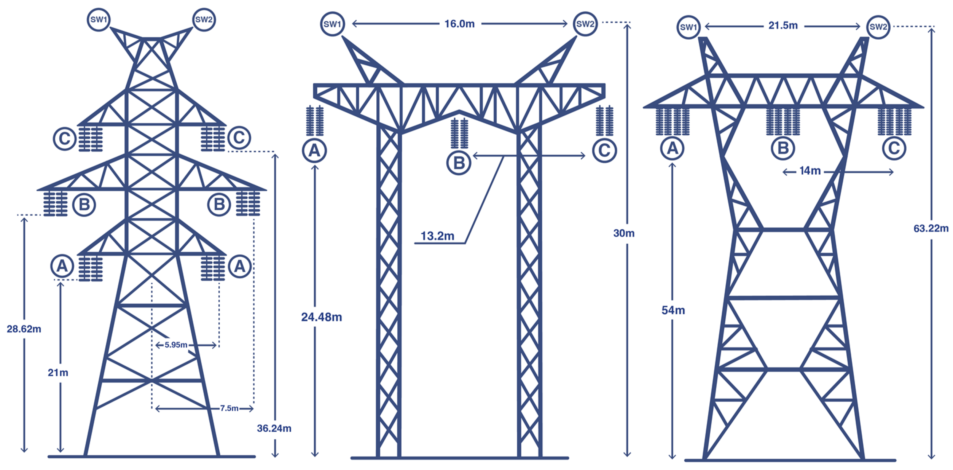
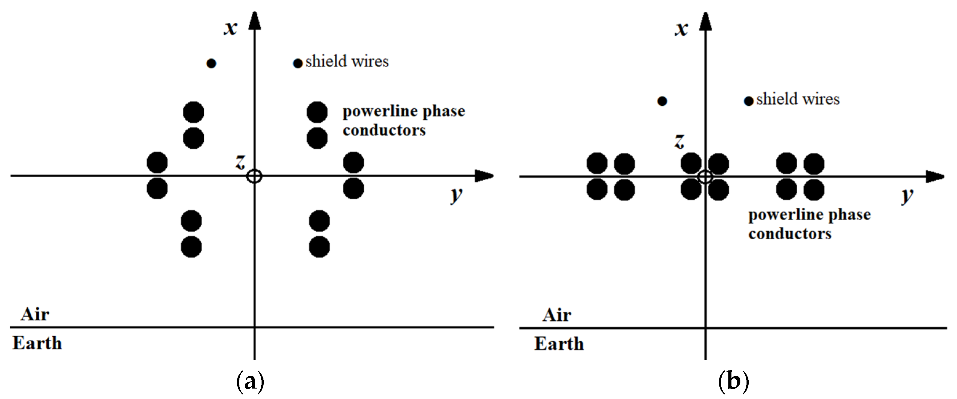
2.1. Model Description
2.2. Electric Field and Magnetic Vector Potential Formulation
2.3. FEM Analysis for the Electric Field Problem
2.4. FEM Analysis for the Magnetic Field Problem
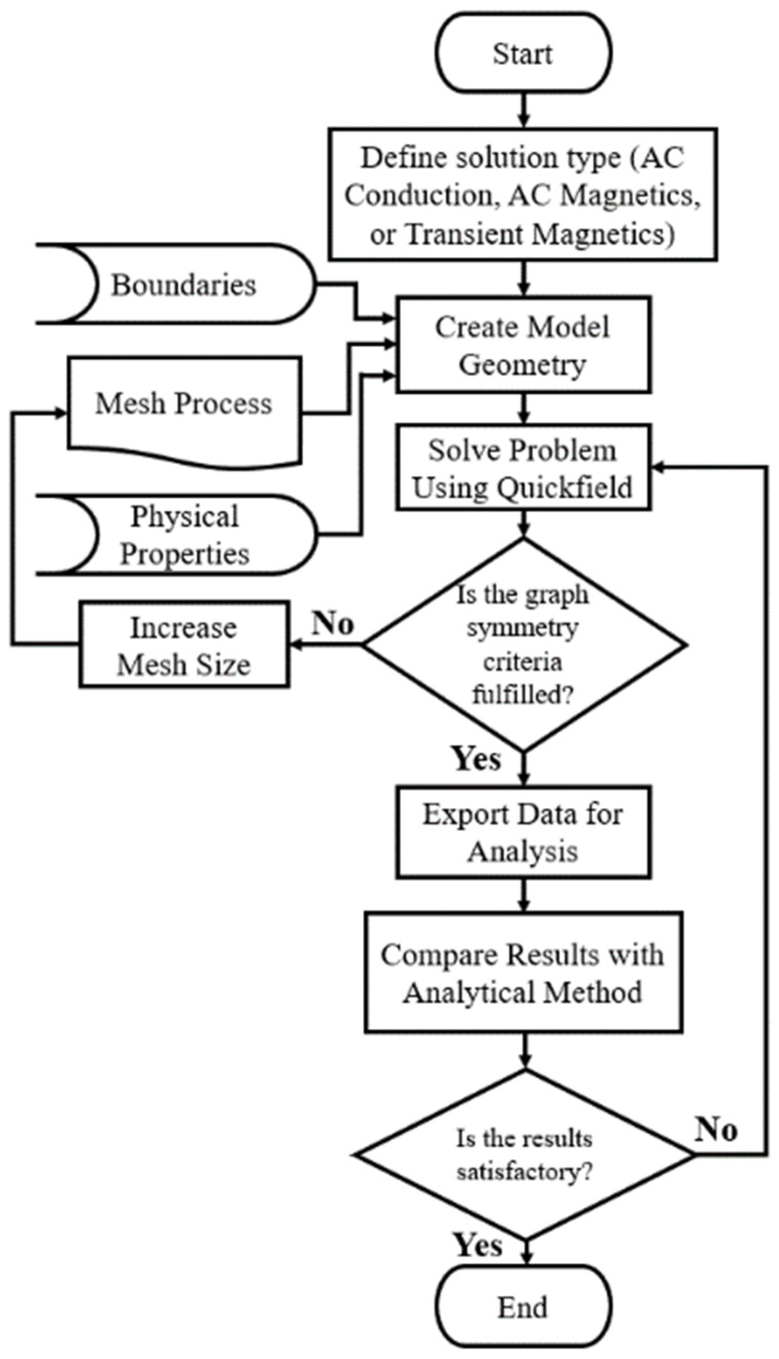
2.5. QuickFiekd Simulation Model Procedures
3. Results and Discussion
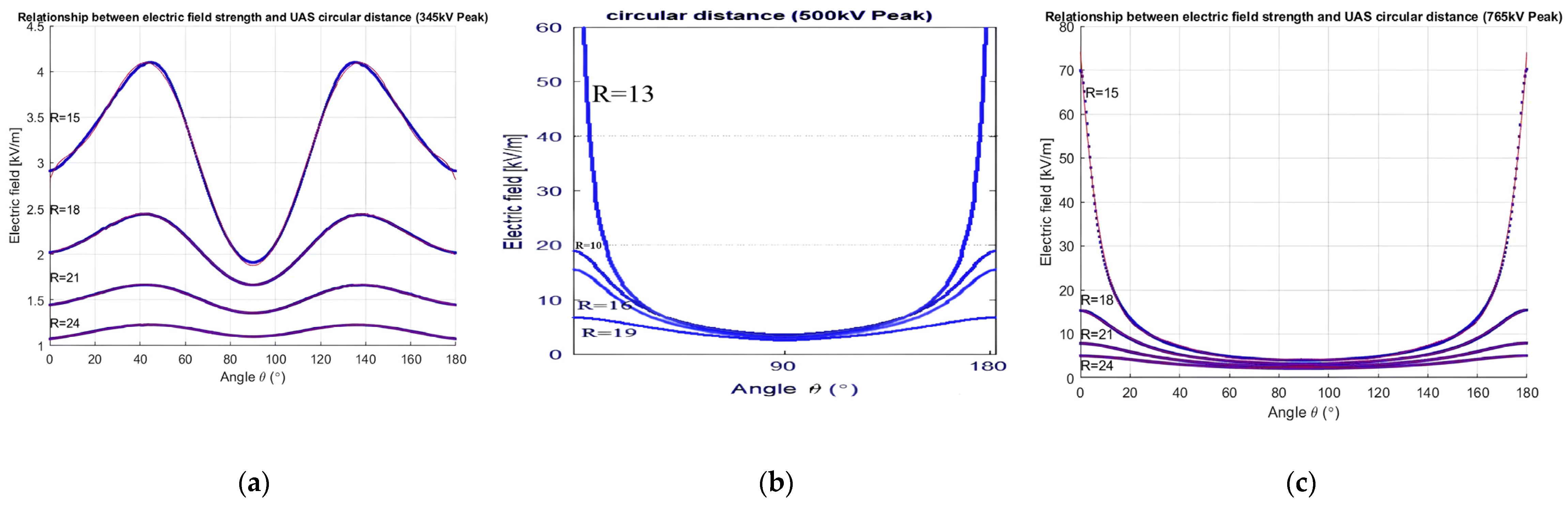
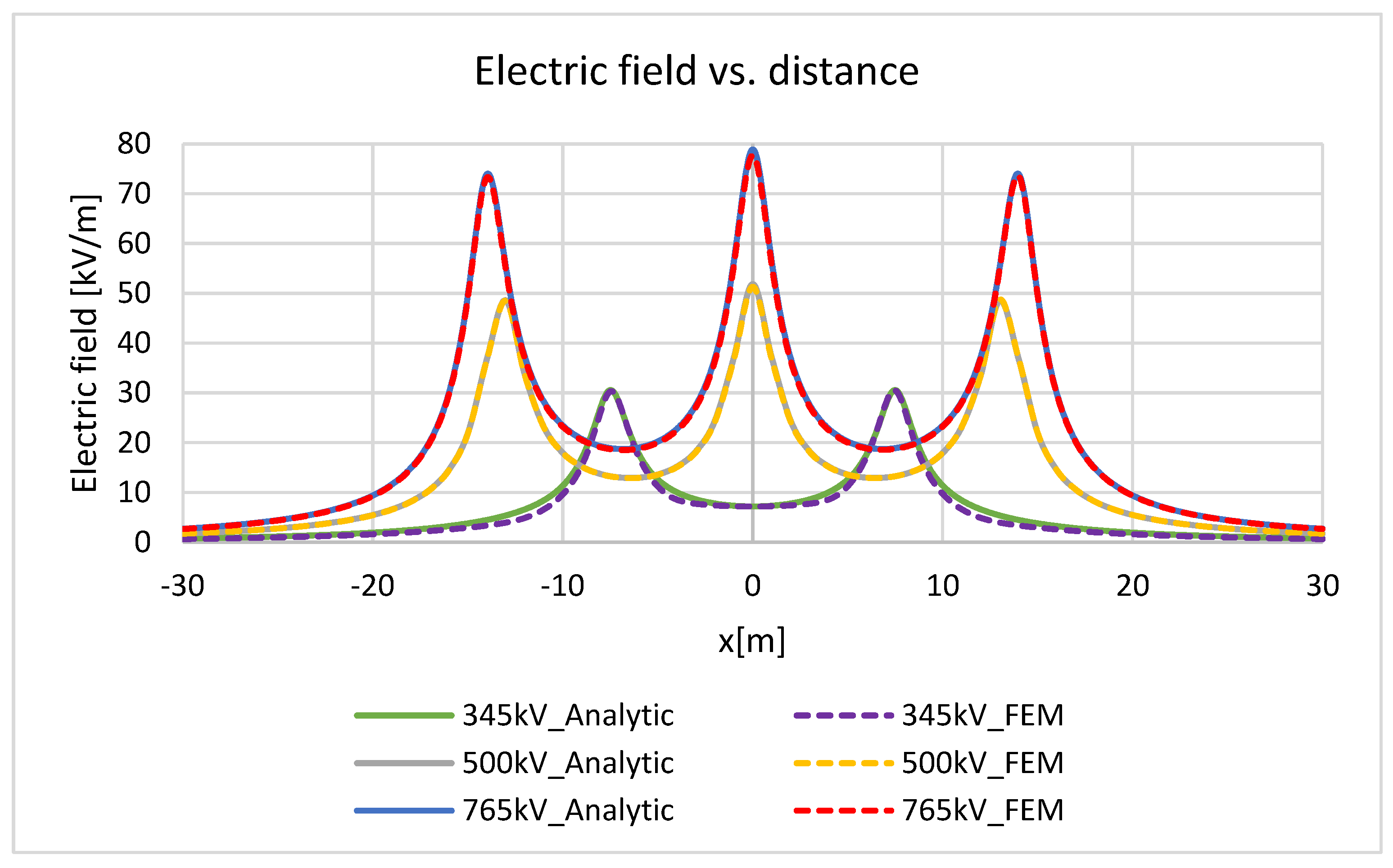
3.1. Electric Field
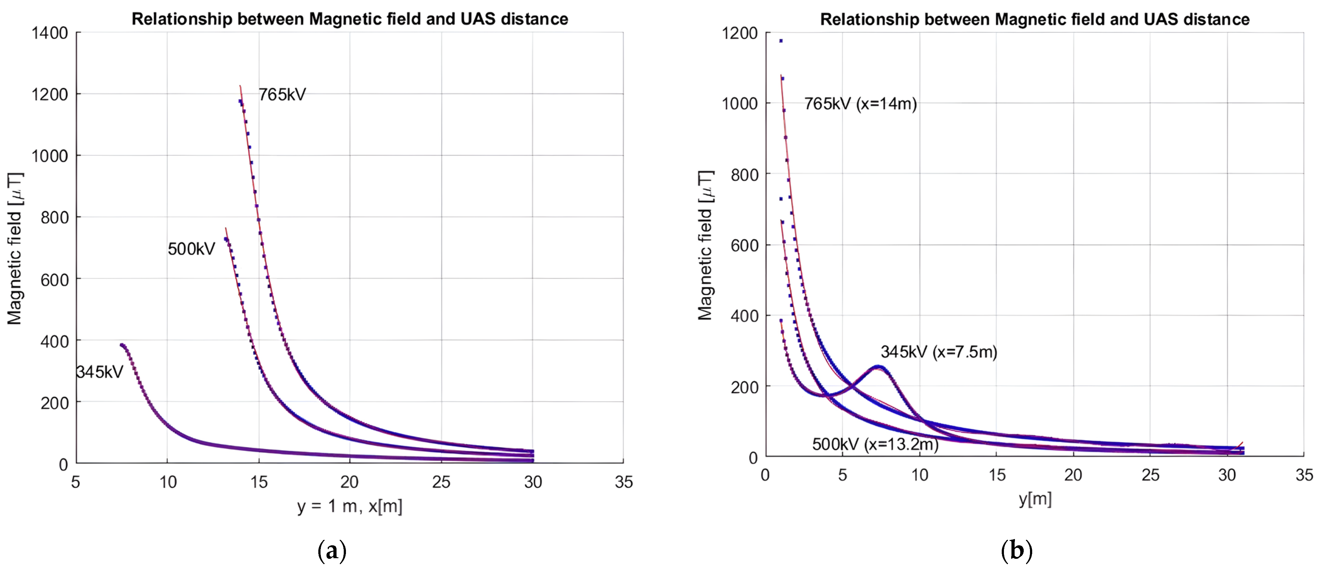
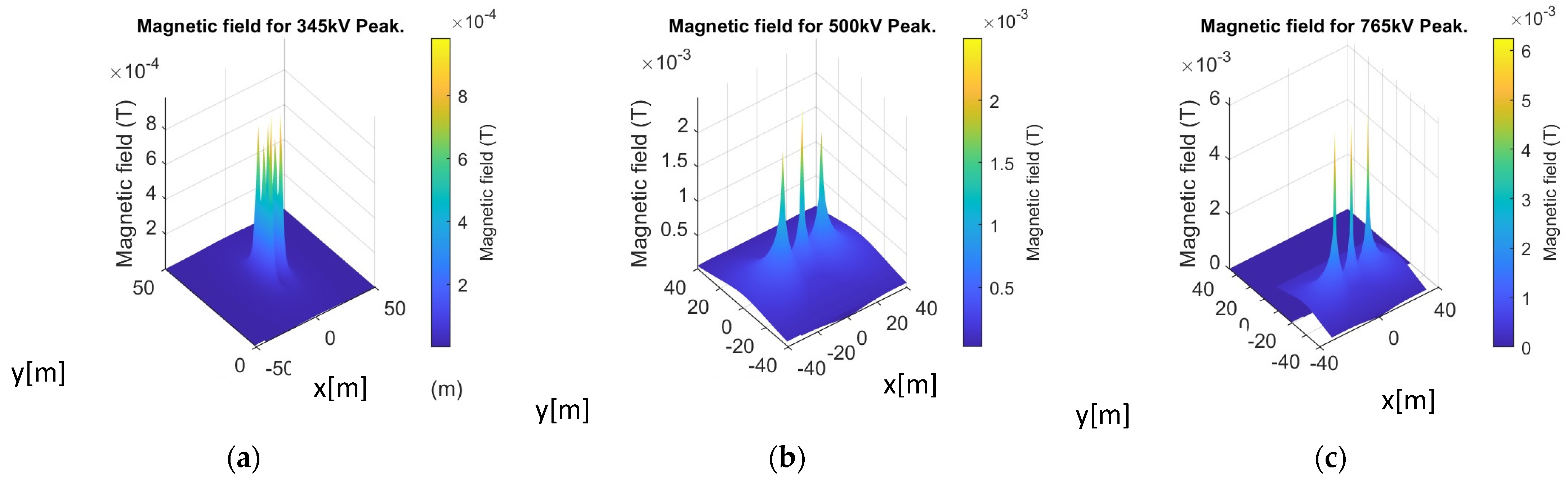
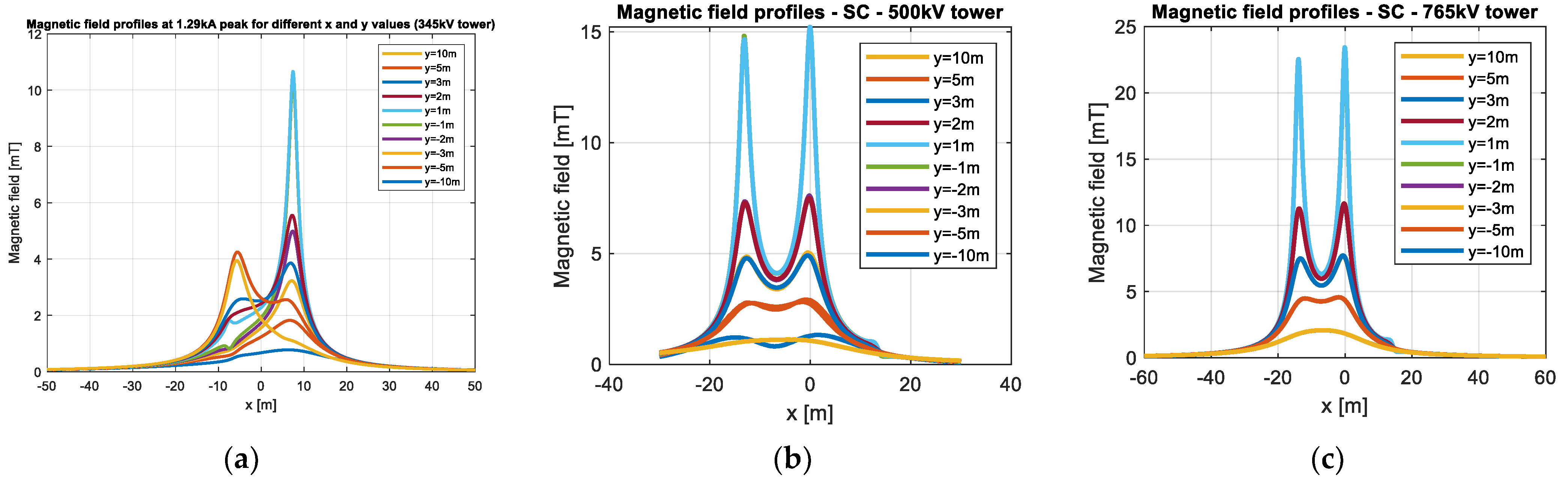
3.2. Magnetic Field
3.3. Minimum Distance Constraints Analysis for UAV Inspection
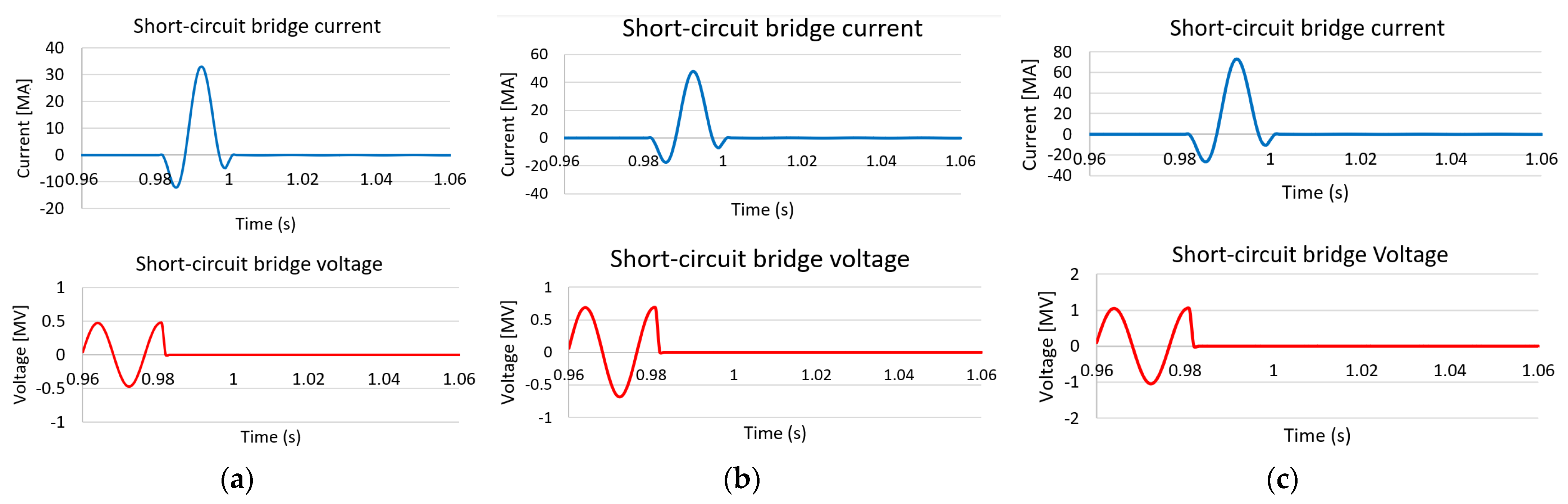
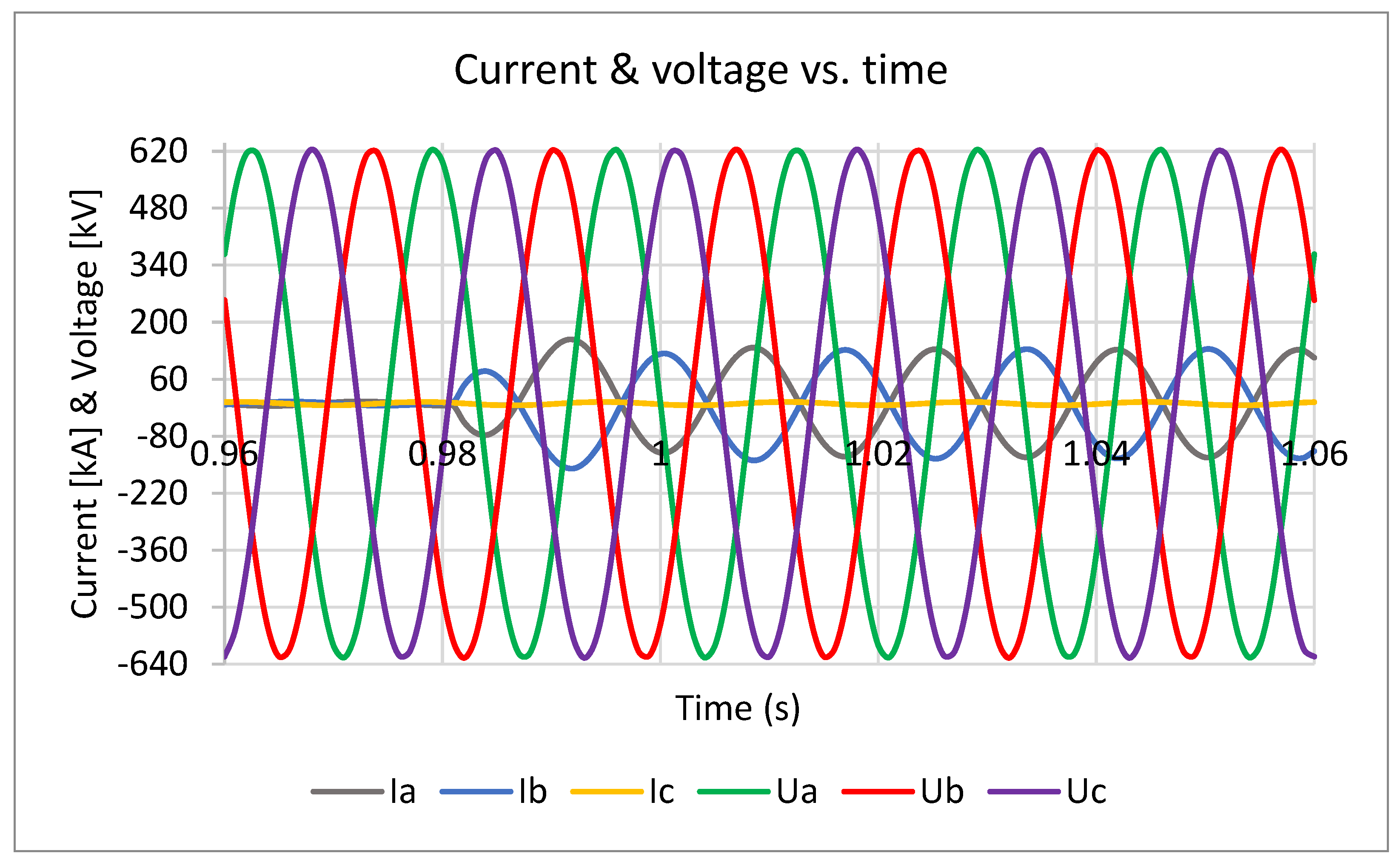
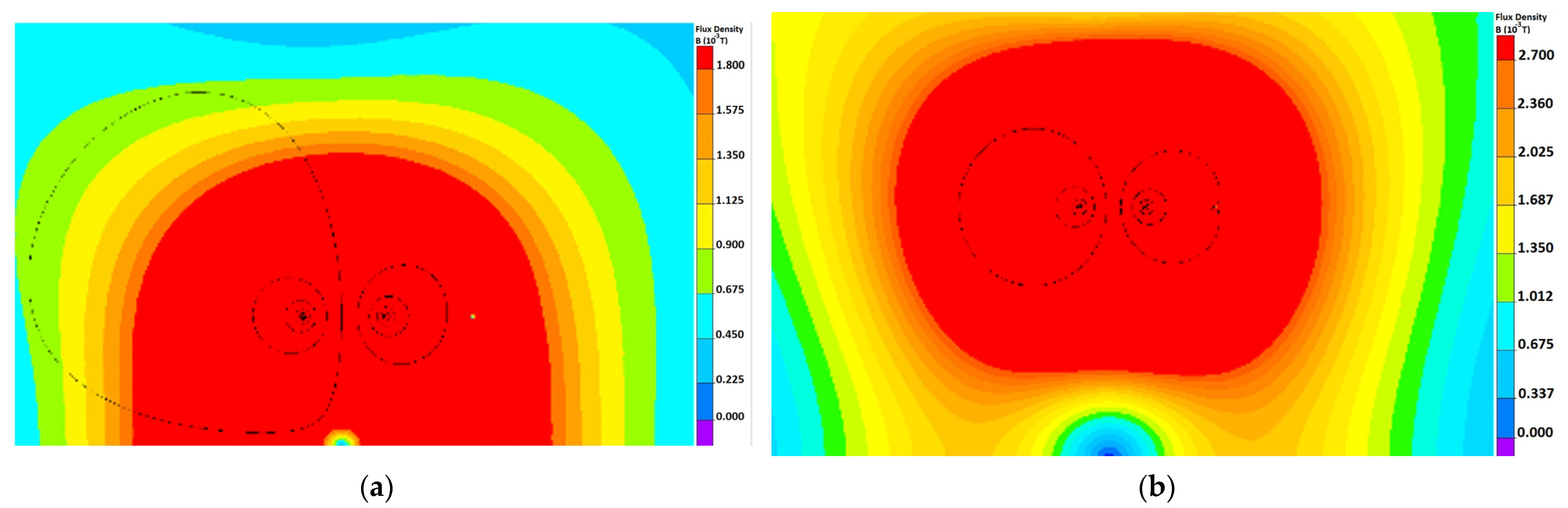
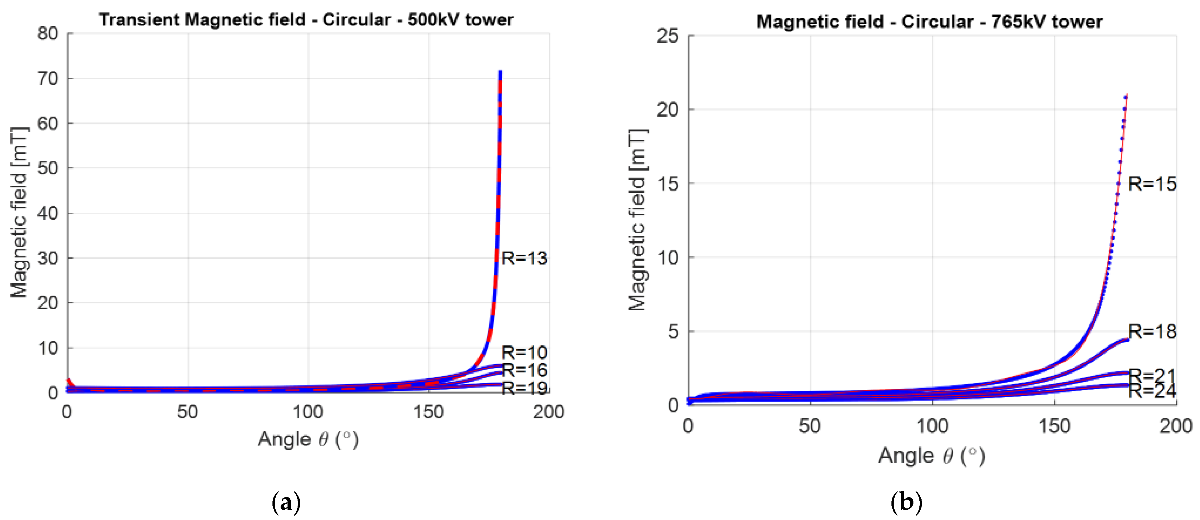
3.4. Transient Magnetic Filed
3.5. Validations of the Results
4. Conclusions
Author Contributions
Funding
Data Availability Statement
Acknowledgments
Conflicts of Interest
References
- Kim, S.-G.; Lee, E.; Hong, I.-P.; Yook, J.-G. Review of Intentional Electromagnetic Interference on UAV Sensor Modules and Experimental Study. Sensors 2022, 22, 2384. [Google Scholar] [CrossRef] [PubMed]
- Zhang, W.; Ning, Y.; Suo, C. A Method Based on Multi-Sensor Data Fusion for UAV Safety Distance Diagnosis. Electronics 2019, 8, 1467. [Google Scholar] [CrossRef]
- National Coordinating Center for Communications (NCC). Electromagnetic Pulse (EMP) Protection and Resilience Guidelines for Critical Infrastructure and Equipment; Version 2.2; National Cybersecurity and Communications Integration Center: Arlington, VA, USA, 2019.
- Lusk, R.M.; Monday, W.H. An Early Survey of Best Practices for the Use of Small Unmanned Aerial Systems by the Electric Utility Industry; Oak Ridge National Laboratory: Oak Ridge, TN, USA, 2017.
- Chen, D.-Q.; Guo, X.-H.; Huang, P.; Li, F.-H. Safety Distance Analysis of 500 kV Transmission Line Tower UAV Patrol Inspection. IEEE Lett. Electromagn. Compat. Pract. Appl. 2020, 2, 124–128. [Google Scholar] [CrossRef]
- Park, J.; Kim, S.; Lee, J.; Ham, J.; Oh, K. Method of operating a GIS-based autopilot drone to inspect ultrahigh voltage power lines and its field tests. J. Field Robot. 2020, 37, 345–361. [Google Scholar] [CrossRef]
- Silva, M.F.; Honório, L.M.; Santos, M.F.; Vidal, V.F.; Mercorelli, P. Model and Validation of the Electromagnetic Interference Produced by Power Transmission Lines in Robotic Systems. In Proceedings of the 2021 25th International Conference on System Theory, Control and Computing (ICSTCC), Iasi, Romania, 20–23 October 2021; pp. 266–271. [Google Scholar]
- da Silva, M.F.; Honório, L.M.; Marcato, A.L.; Vidal, V.F.; Santos, M.F. Unmanned aerial vehicle for transmission line inspection using an extended kalman filter with colored electromagnetic interference. ISA Trans. 2020, 100, 322–333. [Google Scholar] [CrossRef] [PubMed]
- Virjoghe, E.O.; Nescu, D.E.; Stan, M.F.; Cobianu, C. Numerical determination of electric field around a high voltage electrical overhead line. J. Sci. Arts 2012, 4, 487–496. [Google Scholar]
- Boukabou, I.; Foust, L.; Benouadah, S.; Rupanetti, D.; Wolf, J.; Kaabouch, N. Electric Field Around Extra-High Voltage Transmission Lines for UAS Powerline Inspection. In Proceedings of the 2022 North American Power Symposium (NAPS), Salt Lake City, UT, USA, 9–11 October 2022; pp. 1–6. [Google Scholar] [CrossRef]
- Foust, L.; Boukabou, I.; Rupanetti, D.; Benoudah, S.; Kaabouch, N. UAS Safe Distance due to Magnetic Field of Extra High Voltage Transmission Lines during a Phase-to-Phase Short Circuit. In Proceedings of the 2022 North American Power Symposium (NAPS), Salt Lake City, UT, USA, 9–11 October 2022; pp. 1–5. [Google Scholar] [CrossRef]
- Brown, J. Great Northern Transmission Line Project–EMF and Corona Effects Calculations from Appendix I, Memorandum to L. Henriksen; Portland, OR, USA, 2013. [Google Scholar]
- Stangeland, K. Positioning in Electromagnetic Fields. Master’s Thesis, University of Stavanger, Stavanger, Norway, 2015. [Google Scholar]
- Anderson, J.G. Transmission Line Reference Book: 345 kV and Above; Electric Power Research Institute: Palo Alto, CA, USA, 1982. [Google Scholar]
- Switch Gear and Substations, Siemens Energy Sector. Power Engineering Guide, 8th ed.; Erlangen, Germany, 2017. [Google Scholar]
- Lunca, E.C.; Neagu, B.C.; Vornicu, S. Finite Element Analysis of Electromagnetic Fields Emitted by Overhead High-Voltage Power Lines. In Numerical Methods for Energy Applications; Power Systems; Springer International Publishing: Berlin/Heidelberg, Germany, 2021; ISBN 978-3-030-62190-2. [Google Scholar]
- Faiz, J.; Ojaghi, M. Instructive Review of Computation of Electric Fields using Different Numerical Techniques. Int. J. Eng. Educ. 2002, 18, 344–356. [Google Scholar]
- Tera Analysis Ltd. QuickField Finite Element Analysis System; Version 6.3.1 User’s Guide; Tera Analysis Ltd.: Svendborg, Denmark, 2018. [Google Scholar]
- Nigbor, R.J.; Pakala, W.E. A Survey of Methods for Calculating Transmission Line Conductor Surface Voltage Gradients. IEEE Trans. Power Appar. Syst. 1996, PAS-98, 1996–2014. [Google Scholar]
- Finneran, S.; Krebs, B.; Bensman, L. Criteria for Pipelines Co-Existing with Electric Power Lines; The INGAA Foundation: Washington, DC, USA, 2015; Volume 4. [Google Scholar]
- Ayad, A.; Krika, W.; Boudjella, H.; Benhamida, F.; Horch, A. Simulation of the electromagnetic field in the vicinity of the overhead power transmission line. Eur. J. Electr. Eng. 2019, 21, 49–53. [Google Scholar] [CrossRef]
- Fikry, A.; Lim, S.C.; Ab Kadir, M.Z.A. EMI radiation of power transmission lines in Malaysia. F1000Research 2021, 10, 1136. [Google Scholar] [CrossRef] [PubMed]


| Nominal Voltage Level [kV] | 345 | 500 | 765 |
|---|---|---|---|
| Highest system current rating at 80 °C [kA] | 1.29 | 2.58 | 4.16 |
| Frequency [Hz] | 60 | 60 | 60 |
| Phase angle [deg.] | C-C: 0–240 | A: 0 | A: 0 |
| B-B: 120–120 | B: 120 | B: 120 | |
| A-A: 240–0 | C: 240 | C: 240 | |
| Distance between phases and ground [m] | C-C: 5.95 | 24.48 | 54 |
| B-B: 7.5 | |||
| A-A: 5.95 | |||
| Nominal cross-section [mm2] | Bundle | Bundle | Bundle |
| 2 × 240 | 2 × 560 | 4 × 560 | |
| Equivalent radius [mm] | 21.9 | 26 | 32.2 |
| Electric Field Strength [kV/m] | 345 kV | 500 kV | 765 kV |
|---|---|---|---|
| 10 | ≥(2.50, 9.35) | ≥(4.14, 4.58) | ≥(5.74, 6.77) |
| 20 | ≥(1.35, 1.64) | ≥(2.23, 2.49) | ≥(3.16, 3.58) |
| 30 | ≥(0.91, 1.01) | ≥(1.53, 1.69) | ≥(2.2, 2.42) |
| 40 | ≥(0.68, 0.75) | ≥(1.17, 1.28) | ≥(1.69, 1.82) |
| 50 | ≥(0.54, 0.60) | ≥(0.94, 1.03) | ≥(1.37, 1.5) |
| 60 | ≥(0.45, 0.49) | ≥(0.79, 0.86) | ≥(1.16, 1.22) |
| 70 | ≥(0.38, 0.42) | ≥(0.68, 0.74) | ≥(1.0, 1.04) |
| 80 | ≥(0.33, 0.36) | ≥(0.60, 0.64) | ≥(0.88, 0.92) |
| 90 | ≥(0.29, 0.32) | ≥(0.53, 0.57) | ≥(0.76, 0.81) |
| 100 | ≥(0.26, 0.29) | ≥(0.48, 0.56) | ≥(0.71, 0.74) |
| Magnetic Field Intensity [µT] | 345 kV | 500 kV | 765 kV |
|---|---|---|---|
| 100 | ≥(3.06, 10.28) | ≥(6.1, 6.73) | ≥(8.2, 10.35) |
| 120 | ≥(2.65, 9.77) | ≥(5.3, 5.73) | ≥(7.12, 8.85) |
| 140 | ≥(2.34, 9.37) | ≥(4.71, 4.97) | ≥(6.31, 7.74) |
| 160 | ≥(2.07, 9.05) | ≥(4.24, 4.39) | ≥(5.65, 6.88) |
| 180 | ≥(1.90, 8.76) | ≥(3.9, 3.92) | ≥(5.1, 6.2) |
| 200 | ≥(1.71, 8.48) | ≥(3.56, 3.56) | ≥(4.7, 5.6) |
| 220 | ≥(1.56, 8.19) | ≥(3.3, 3.24) | ≥(4.34, 5.13) |
| 240 | ≥(1.44, 7.87) | ≥(3, 2.99) | ≥(4.03, 4.73) |
| 260 | ≥(1.34, 1.59) | ≥(2.9, 2.77) | ≥(3.77, 4.39) |
| 280 | ≥(1.25, 1.45) | ≥(2.74, 2.57) | ≥(3.53, 4.09) |
| Magnetic Field Intensity [µT] | 345 kV | 500 kV | 765 kV |
|---|---|---|---|
| 100 | ≥(34.86, 45) | ≥(19.53, 36.01) | ≥(25.8, 45.2) |
| 120 | ≥(30.77, 40.63) | ≥(22.11, 32.36) | ≥(29.33, 42.15) |
| 140 | ≥(27.42, 37.57) | ≥(24.91, 30.42) | ≥(33.01, 39.29) |
| 160 | ≥(24.87, 35.03) | ≥(27.21, 28.76) | ≥(36.33, 37.29) |
| 180 | ≥(22.74, 33.11) | ≥(29.2, 27.11) | ≥(39.4, 35.62) |
| 200 | ≥(20.91, 36.01) | ≥(30.93, 31.47) | ≥(42.08, 34.09) |
| 220 | ≥(19.3, 30) | ≥(32.42, 24.95) | ≥(44.28, 32.8) |
| 240 | ≥(17.91, 28.76) | ≥(33.76, 23.97) | ≥(46.22, 31.54) |
| 260 | ≥(16.78, 27.68) | ≥(34.91, 23.06) | ≥(47.9, 30.45) |
| 280 | ≥(15.7, 26.71) | ≥(35.95, 22.26) | ≥(49.34, 29.43) |
Disclaimer/Publisher’s Note: The statements, opinions and data contained in all publications are solely those of the individual author(s) and contributor(s) and not of MDPI and/or the editor(s). MDPI and/or the editor(s) disclaim responsibility for any injury to people or property resulting from any ideas, methods, instructions or products referred to in the content. |
© 2024 by the authors. Licensee MDPI, Basel, Switzerland. This article is an open access article distributed under the terms and conditions of the Creative Commons Attribution (CC BY) license (https://creativecommons.org/licenses/by/4.0/).
Share and Cite
Boukabou, I.; Kaabouch, N. Electric and Magnetic Fields Analysis of the Safety Distance for UAV Inspection around Extra-High Voltage Transmission Lines. Drones 2024, 8, 47. https://doi.org/10.3390/drones8020047
Boukabou I, Kaabouch N. Electric and Magnetic Fields Analysis of the Safety Distance for UAV Inspection around Extra-High Voltage Transmission Lines. Drones. 2024; 8(2):47. https://doi.org/10.3390/drones8020047
Chicago/Turabian StyleBoukabou, Issam, and Naima Kaabouch. 2024. "Electric and Magnetic Fields Analysis of the Safety Distance for UAV Inspection around Extra-High Voltage Transmission Lines" Drones 8, no. 2: 47. https://doi.org/10.3390/drones8020047