Abstract
UAV rotors are at a high risk of ice accumulation during their operations in icing conditions. Thermal ice protection systems (IPSs) are being employed as a means of protecting rotor blades from ice, yet designing the appropriate IPS with the required heating density remains a challenge. In this work, a reduced-order modeling technique based on the Unsteady Vortex Lattice Method (UVLM) is proposed as a way to predicting rotor icing and to calculate the required anti-icing heat loads. The UVLM is gaining recent popularity for aircraft and rotor modeling. This method is flexible enough to model difficult aerodynamic problems, computationally efficient compared to higher-order CFD methods and accurate enough for conceptual design problems. A previously developed implementation of the UVLM for 3D rotor aerodynamic modeling is extended to incorporate a simplified steady-state icing thermodynamic model on the stagnation line of the blade. A viscous coupling algorithm based on a modified α-method incorporates viscous data into the originally inviscid calculations of the UVLM. The algorithm also predicts the effective angle of attack at each blade radial station (r/R), which is, in turn, used to calculate the convective heat transfer for each r/R using a CFD-based correlation for airfoils. The droplet collection efficiency at the stagnation line is calculated using a popular correlation from the literature. The icing mass and heat transfer balance includes terms for evaporation, sublimation, radiation, convection, water impingement, kinetic heating, and aerodynamic heating, as well as an anti-icing heat flux. The proposed UVLM-icing coupling technique is tested by replicating the experimental results for ice accretion and anti-icing of the 4-blade rotor of the APT70 drone. Aerodynamic predictions of the UVLM for the Figure of Merit, thrust, and torque coefficients agree within 10% of the experimental measurements. For icing conditions at −5 °C, the proposed approach overestimates the required anti-icing flux by around 50%, although it sufficiently predicts the effect of aerodynamic heating on the lack of ice formation near the blade tips. At −12 °C, visualizations of ice formation at different anti-icing heating powers agree well with UVLM predictions. However, a large discrepancy was found when predicting the required anti-icing heat load. Discrepancies between the numerical and experimental data are largely owed to the unaccounted transient and 3D effects related to the icing process on the rotating blades, which have been planned for in future work.
1. Introduction
In-flight icing is a major hazard for all types of aircraft, rotorcraft, and UAV manufacturers and is a cause of major concern for the certification authorities [1,2]. The last decade saw a huge influx towards the use of unmanned aerial vehicles (UAVs) and drones for a wide variety of military, commercial, and recreational applications [3]. Most of the small- or medium-sized UAVs use some form of propellers for propulsion and are driven by an electrically powered motor with an onboard battery [4]. Rotary wing UAVs are more sensitive to icing conditions compared to fixed wings, mainly due to the high speeds of rotation, their small size, and the limited electrical power capacity their battery can store [2]. Recent experimental studies have shown that a 2 min exposure to severe icing conditions is enough to cause a 50% reduction in thrust and motor power losses of up to 100% [5]. Icephobic coatings are being tested as a possible means of preventing ice accretion [6,7], yet thermal IPSs have been long considered, and continue to be, the most reliable IPS for rotors [8]. They work by converting electrically supplied energy into heat, which keeps the rotor surfaces warm enough to prevent ice formation [9].
The advances in computational capabilities and technologies led to the development of numerous international icing codes, such as LEWICE [10], ONERA [11], FENSAP-ICE [12], and CANICE [13]. Until around 2005, the focus of developed icing codes was mainly around fixed wing aircraft, mainly driven by NASA, re-prioritizing its plans and halting rotorcraft icing research in 1994 due to a need to focus on fixed wing analyses following a number of high-profile passenger aircraft crashes due to icing [14]. LEWICE later became an industry standard for fixed wing analyses with a large database of validated test cases, ice shapes, and anti-icing scenarios [15]. Today, high-fidelity icing codes using CFD and fully resolved RANS equations for rotorcraft have been studied and developed [16,17,18] but remain limited by one or more of the following main disadvantages: (1) lack of extensive validation data and sometimes inaccurate results, especially for rotorcraft; (2) setup complexity (requirement of specific software, meshing, boundary condition application, post-processing etc.); (3) the need for high-performance computing to run the simulations; and (4) grid-induced dissipation errors due to the numerical discretization over the flow field that may result in a rapid decay of the intensity of the rotor tip vortex downstream and a breakdown of the helical rotor wake structure [19].
On the other hand, manufacturers need to design UAVs that satisfy the specific needs of various areas of markets and applications [3]. The latter requires the design of all types of weights, rotor speeds, sizes, geometries, and operating conditions. Predictions of thrust and torque generation, motor power requirements, and anti-icing power needs are all parameters that are looked at, among many others [4]. Moreover, during the conceptual phase of each of these designs, manufacturers go through many different versions where one or more design variables are iterated on until the final agreed upon design gets promoted to undergo further evaluation and analysis. It will therefore be practically impossible to run high-fidelity analyses for each iteration of each design since computational requirements and simulation times will grow exponentially.
For these reasons, manufacturers are interested in developing reliable software that can provide reasonable predictions in a computationally inexpensive way and quick simulation time. These kinds of numerical tools would not match the accuracy of full-fledged CFD simulations but could provide a faster prediction of the required parameters without the need for high-performance computing and within a reasonable accuracy that is suitable for a conceptual design.
An excellent example of these numerical tools is based on the Unsteady Vortex Lattice Method (UVLM), which has been more and more regarded as a reduced-order modeling method that can provide acceptable and accurate results for complex configuration designs in less time than the CFD-based methods [20]. According to a recent review [21], the UVLM has had a renewed interest in the past decade and is preferred over other potential flow-solvers due to its low-order, quick, and highly efficient computational analysis. This review covered around 150 state-of-the-art recently published studies where the UVLM has been used to model the steady, unsteady, linear, and non-linear aerodynamics of subsonic and supersonic aircraft on all sorts of wing and rotor blade planforms. For rotor-specific considerations, another recent review sheds light on the potential of the UVLM in studying rotor aerodynamics, aeroacoustics, and aeroelastics [19].
In a previous publication, a UVLM-based numerical tool to model the aerodynamics and compute the convective heat transfer on rotor blades was presented [22]. It can simulate multi-blade rotors, variable blade geometries (airfoil shape, chord, twist etc.), rotors in ground effect, and operations in hover, axial, or forward flight. This tool includes viscous and heat transfer effects via multi-layered non-linear coupling to a 2D CFD viscous database and a 2D CFD heat transfer correlation obtained using high-fidelity CFD simulations for airfoils [23].
In this work, this tool is extended to predict the required anti-icing heat requirement for rotors in the case when a thermal ice protection system is used. The numerical approach towards 3D aerodynamic modeling is first presented. Next, the algorithm used to incorporate sectional viscous data is laid out, along with the methodology used for the convective heat transfer calculation. The collection efficiency estimation, together with the simplified icing model, is then discussed. The results are focused on simulating the experimental setup of a rotor with heated blades from a previous experimental campaign and comparing the numerical and experimental data.
2. Materials and Methods
2.1. Background and Inspiration
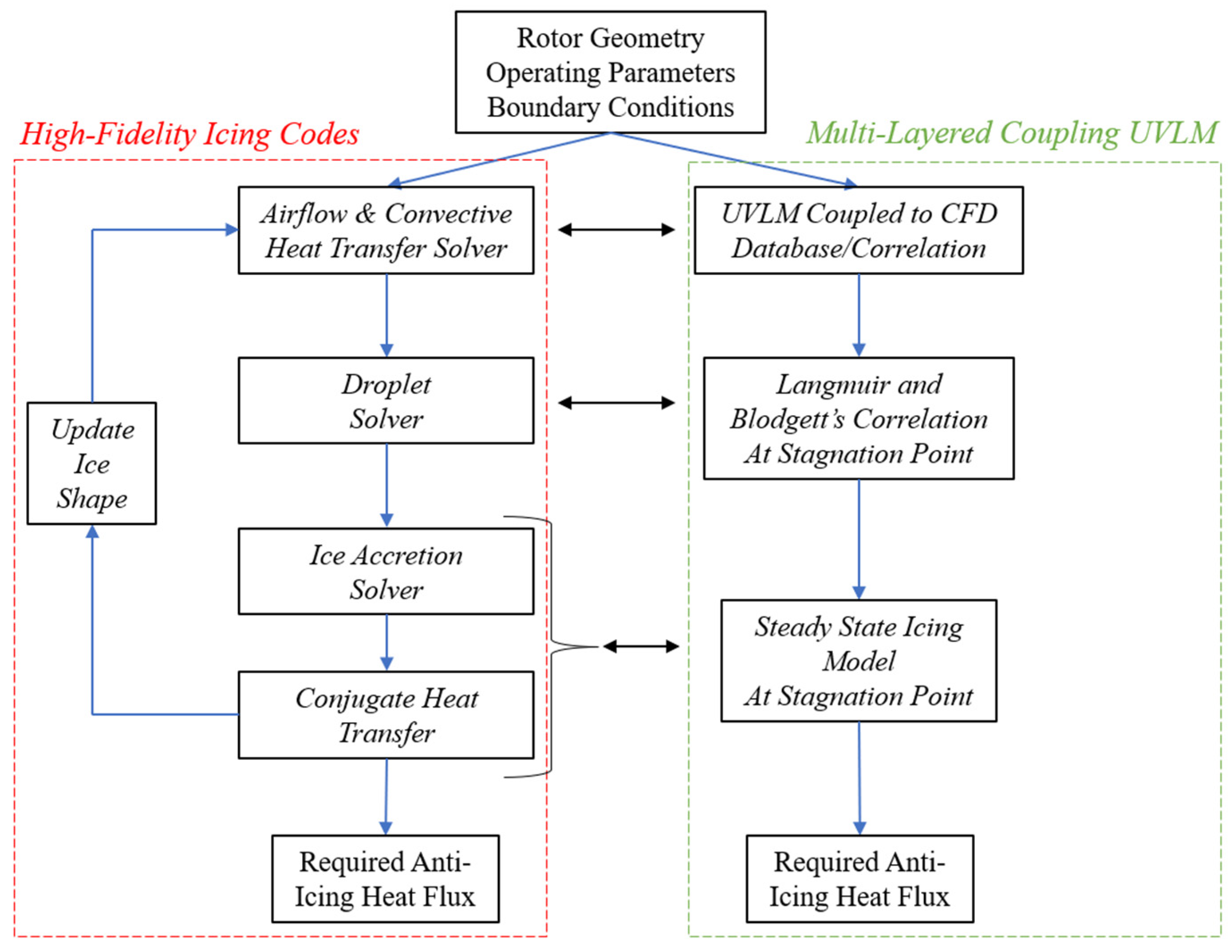
The numerical tool developed in this paper was inspired by the structure of the state-of-the-art icing codes. The geometry, operating parameters (rotor speed, pitch, and twist), and icing conditions, such as the liquid water content (LWC), median volume droplet (MVD), and air temperature (T∞), must be known prior to meshing and for the model boundary condition setup. The general architecture of icing codes is typically composed of four different solvers that are described in the sequence shown in Figure 1 [24]. In the airflow solver, the external aerodynamics of the blade are modeled, and the surface convective heat transfer () is calculated. Usually, a potential flow-based method or a higher-order RANS model are used for this approach. For the droplet solver, the collection efficiency (β0) of the impinging water droplets that have a possibility of freezing on the blade is determined, as well as its freezing position. The droplet trajectory analysis is either calculated using the Eulerian or Lagrangian approaches. In the ice accretion solver, the water mass and energy balance equations are applied within the viscous layer at the solid surface. Many methods have been developed for this approach, most notably the Messinger Model, Extended Messinger Model, Iterative Messinger Model, or Shallow Water Icing Model (SWIM). A comparative assessment of these models can be found in [25]. Finally, for the conjugate heat transfer solver, the effect of the internal heat generated by a thermal IPS is transferred to the mass and energy balance equations by a conductive heat transfer term. The heat generated could originate from an electric resistance buried inside a multi-layered airfoil surface [26] or through a hot air anti-icing system [13]. The four solvers operate sequentially and iteratively at all discretized control volumes (CVs) of the analyzed 2D airfoil or 3D wing or blade. The main result of this scheme is to predict a freezing fraction term, ff, that represents the amount of frozen water compared to the total water mass, which is, in turn, used to predict the ice thickness normal to each CV’s surface [27]. For unsteady analyses, a time-stepping approach is used to model the ice growth throughout the simulated icing time [28].
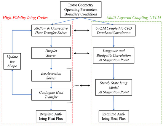
Figure 1.
Architecture of typical high-fidelity icing codes compared to their simplification, followed by the multi-layered coupling UVLM.
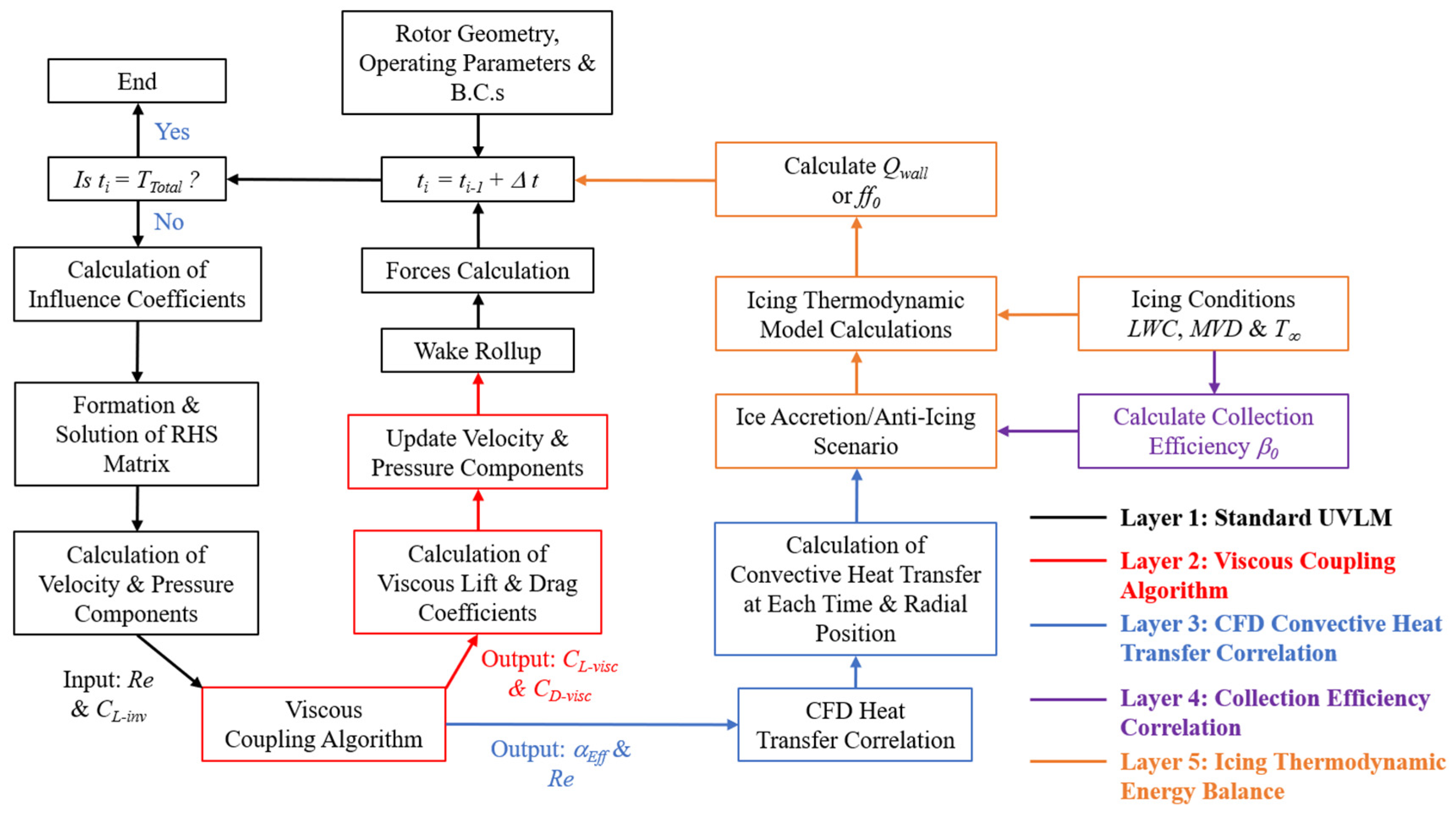
In this paper, a new and simplified methodology based on the UVLM is proposed to model ice accretion anti-icing for rotors, as presented in Figure 2. A multi-layered coupling scheme was applied to the Unsteady Vortex Lattice Method (UVLM) for rotors. Four coupling layers were proposed as a simplification of the higher-order solvers presented earlier and are as follows: airflow solver simplification: the 3D UVLM for rotors was solved with the incorporation of 2D viscous data for two reasons: (1) to enhance its aerodynamic prediction capabilities by involving the viscous lift and drag coefficients; and (2) to implement a viscous coupling algorithm that predicts the effective angle of attack (αeff) at each azimuthal (Ψ) and r/R of the blades. The UVLM-predicted Reynold’s number, Re, and αeff were then used with a Nusselt number (Nu) correlation for 2D airfoils to obtain at each α and r/R. Droplet solver simplification: the steady-state β0 at the stagnation point (S0) of each r/R was calculated using a renowned correlation from the literature. Ice accretion solver simplification: a steady-state icing thermodynamic model based on a modified version of the Messinger Model [29] was solved at S0 to obtain the freezing fraction. Conjugate heat transfer solver simplification: the steady-state mass and energy conservation equations at S0 were solved to obtain the required anti-icing heat flux for the zero freezing fraction.

Figure 2.
Summarized sequential scheme of the proposed UVLM icing multi-layered coupling approach.
The choice of only applying the droplet and thermodynamic analyses at S0 is justified by two reasons: (1) the availability of previously validated correlations for β0 calculations; (2) the simplifications brought to the icing thermodynamic model at S0 since the only incoming water term is the one from the impinging water droplets (no water runback from other CVs); and (3) most importantly, the stagnation point is typically the location where the highest β0 [30] and highest are observed [31], making it the location of thickest ice accretions and highest requirements of anti-icing heat fluxes. The main drawback of this approach, however, is possibly the over-estimation of the actual ice shapes or since both β0 and are known to dimmish very rapidly within ±5% of S0 [31].
2.2. Unsteady Vortex Lattice Method for Rotor Heat Transfer (UVLM-RHT)
The UVLM-RHT is a medium-fidelity numerical tool that was developed at the École de Téchnologie Supérieure to specifically model the flow around rotor blades and estimate the convective heat transfer on them [22]. Based on the UVLM presented by Katz and Plotkin [32], it is capable of simulating multi-blade rotors, variable blade geometries (airfoil shape, chord, twist etc.), rotors in ground effect, and rotors in hover, axial, or forward flight. It was later developed to include viscous effects by means of coupling the UVLM to a 2D CFD viscous database using a viscous coupling algorithm. The UVLM-RHT also benefits from coupling to a large database of 2D airfoil heat transfer data obtained using high-fidelity CFD simulations on airfoils.
2.2.1. UVLM Basics
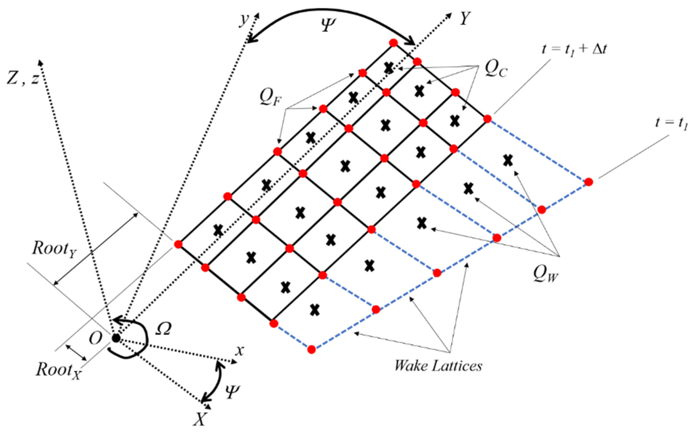
The lattices are placed on the blade’s camberline (forming the corner points QF), as shown in Figure 3. The leading segment was placed on the panel’s 1/4 chord line and the collocation point, QC, at the center of the 3/4 chord line, where the normal vector (nk) was defined. For each timestep Δt, the blade rotates by an azimuth angle (Ψ), and a new row of wake panels is shed from the trailing edge (TE) and freely convected. The center of the shed wake panels was placed at a distance equal to 30% of the length of the shed wake [32]. To enforce the Kutta condition, each shed wake panel carries the same circulation (Γ) as the blade’s TE lattice and remains constant throughout the analysis.

Figure 3.
Vortex lattice distribution on a blade with shed wake lattices.
The Lamb–Oseen viscous core model [33], given by Equation (1), is used to correct the singularities of the Biot–Savart law equation that is typically used in standard UVLM applications. This correction is necessary to avoid numerical instabilities when the distance between a straight-line vortex element and an evaluation point becomes small, which may cause artificially large wake displacements, especially in the region near the hub [22,34]. The core size (rc) is given in Equation (2) and accounts for the weakening of a vortex circulation with time due to viscous diffusion based on the model by [35]. ξ is the Oseen parameter (ξ = 1.25643); ν is the static viscosity; t is the time; and a = 10−4 is determined empirically.
The influence coefficients of the blade vortex rings are stored in the aK,L matrix (Equation (3)), where the counters K and L are defined by K = 1→I × J and L = 1→I × J, respectively. The influence coefficients are calculated for each QC and represent the velocities induced due to the influence of all other blade bound vortex lattices (u, v, and w). The RHS matrix was formed by enforcing the zero normal velocity boundary condition on the surface of the blade, and the resulting form is shown in Equation (4). U(t), V(t), and W(t) are the time-dependent kinematic velocity components, whereas uw, vw, and ww terms are the induced velocity components due to the wake lattices. The solution matrix was then set up and solved (Equation (5)).
The pressure difference across the blade was calculated for the fluid dynamic loads by using the Bernoulli equation (Equation (6)). Δb and Δc are the spanwise and chordwise lengths of the lattices, respectively. τi and τj are each panel’s tangential vectors. The force contribution of each lattice in the body’s three axes was then described by Equation (7), where ΔS is the area of each lattice. The thrust and torque coefficients as well as the Figure of Merit (FoM) were then calculated using Equations (8)–(10), respectively.
A slow-starting method proposed by [36] was implemented to avoid numerical instabilities that arise when free-wake models are used for rotor simulations, starting from rest. A Prandtl–Glauert compressibility correction factor [37] was used to correct the circulation terms and include compressibility effects [38]. More details on the developed UVLM for rotor modeling and its modifications can be found in [22].
2.2.2. The Viscous Coupling Algorithm
The viscous coupling algorithm used in this work was the Van Dam α model [22] that was modified by Gallay [21] to remove the dependency of the viscous slope in the coupling algorithm. This was achieved by adapting the collocation points to reflect a slope of CLα = 2π. αeff was first obtained using the inviscid sectional lift coefficient (CL-inv) computed with the Kutta–Joukowski theorem. CL-inv was then interpolated for each αeff in the viscous database until the criteria |CL-inv − CL-visc| > ε was met, where ε = 10−4. The sectional lift was then used to update the UVLM sections’ angle of attack Algorithm 1.
| Algorithm 1 Modified α-based Viscous Coupling Algorithm [39]. | |||
| Viscous Coupling Algorithm | |||
| Solve the inviscid UVLM and obtain CL,inv at all radial positions for each radial position | |||
| While | |||
| 1 | Calculate the effective angle of attack αEff | ||
| 2 | Interpolate the viscous lift CL,visc at αEff from the viscous database | ||
| 3 | Update with relaxation factor ε the viscous correction angle | ||
| end | |||
| end | |||
2.2.3. Convective Heat Transfer Calculation
The heat transfer data used with the UVLM in this work were derived from the 2D CFD Reynolds-averaged Navier–Stokes (RANS) simulations ran using SU2 [40], which have been reported and validated in an earlier publication [23]. The compressible RANS flow equations were solved with the fully turbulent Spalart–Allmaras turbulence model [41] to compute the heat transfer and temperature at the airfoil wall, with the fluid model set to air. The grid used was obtained from NASA [42]; multiple grids that varied from coarse to fine were assessed, and the results of the finest one were used in this paper. The grid has 897 × 257 nodes (counting 257 points on the airfoil surface), while the space at the wall was y/c = 2 × 10⁻⁶, which resulted in y+ ≈ 0.1~0.2. The airfoil wall was discretized into 513 points, with the locations of each point in the domain in the x and y directions known. The location on the airfoil wall was defined by the non-dimensional curvilinear distance S/c, which was calculated using Equation (12). A positive sign was adopted for the S on the upper surface, and a negative sign indicated that the S is considered on the bottom surface.
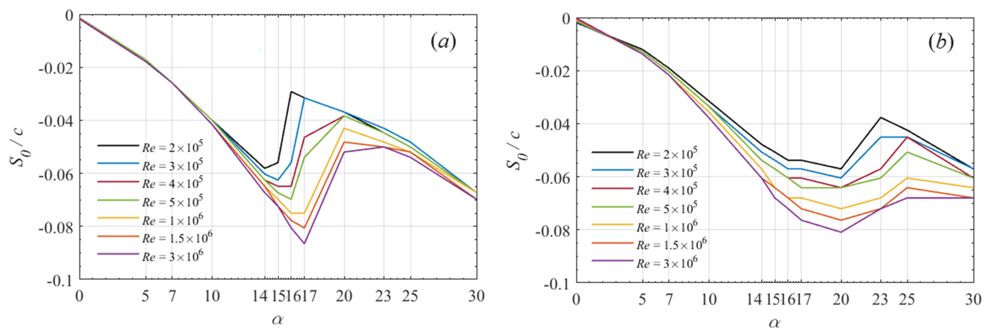
The location of the stagnation point S0 on the airfoil wall was tracked, as shown in Figure 4, as it moved away from the leading edge (LE) and towards the TE as a result of an increasing α for each Re. S0 was identified from the CFD results whenever the pressure coefficient Cp in the LE region was equal to one. Figure 4a depicts the NACA 0012 simulations, and Figure 4b illustrates the NACA 4412 simulations. Depending on the Re used, S0 consistently moved away from the LE up until a range of 0° < α < 17°. For higher α values, the trend is abrupted, and S0 moves back towards the LE. This phenomenon occurs due to flow separation occurring further downstream of the airfoil, as was previously explained in [43]. While this trend agrees with previous experimental and numerical studies, a complete validation of S0 values for the corresponding Re and α of this work was not conducted since the main interest of this work is the convective heat transfer values.
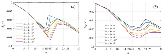
Figure 4.
Stagnation point location on the airfoil wall S0 as a function of Re and α for (a) NACA 0012 and (b) NACA 4412.
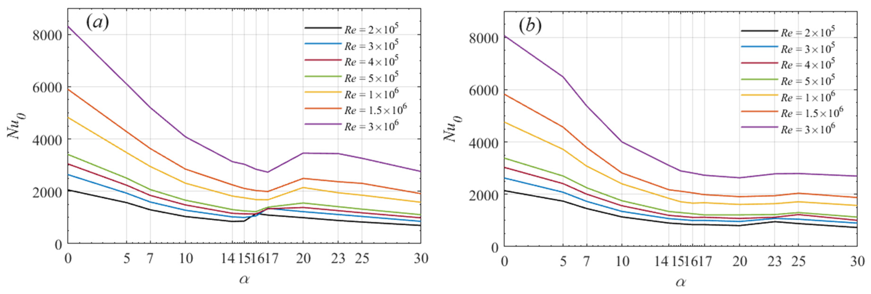
Figure 5 shows the variation in the stagnation point Nusselt number Nu0 that was calculated at each S0 using Equation (12). The convective heat transfer coefficient hc was calculated using Equation (13), where is the convective heat flux; Tsurf is the surface temperature of the airfoil wall; and Trec is the recovery air temperature given by Equation (14). Correlations for the Nu0 for each of the two airfoils were then formed using a curve fitting method and are given by Equation (15) for NACA 0012 and Equation (16) for NACA 4412.

Figure 5.
Stagnation point Nusselt number Nu0 as a function of Re and α for (a) NACA 0012 and (b) NACA 4412.
2.3. Droplet Collection Efficiency
The stagnation line collection efficiency β0 is given by Equation (17) [44]. K0 denotes Langmuir and Blodgett’s expression for the modified inertia parameter, as presented in Equation (18). This formulation for K0 was experimentally determined based on the measurements for cylinders but is widely popular and extensively validated for use on airfoils and rotors [30,45]. Equation (18) is valid for K > 1/8, where K is the inertia parameter given by Equation (19). For K < 1/8, no impingement will occur on the surface. For simplicity, β0 was assumed to remain constant in this work, although it changes with icing shape developments, which is valid if the icing time is kept deliberately small (<2 min) to avoid significant changes to β0 as the ice shape develops [45].
is defined as the dimensionless droplet range parameter and is calculated using Equation (20); rLE is the leading edge radius of the airfoil; and is the droplet-specific Reynold’s number and is calculated based on the MVD.
2.4. The Icing Thermodynamic Model
In the following sections, the heat and mass transfer balance used in this work are presented. The analysis based on the 2D Messinger thermodynamic model is presented [29]; however, simplifications were introduced to account for the preliminary approach this paper uses towards icing and the calculation of the required anti-icing heat load. Mainly, the droplets’ temperature and velocity are assumed to be equal to that of the freestream (Td = T∞), and the temperature within the water and ice layer is constant and set to the freezing temperature of water (Tsurf = Tfr = 0 °C). Together with the steady-state icing approach, these assumptions neglect the effects of surface roughness as well as the water and ice thickness on the airfoil surface. While these assumptions have been used in past works and provided acceptable results [25,30], they are known to produce inaccuracies and errors in the predicted ice shape. For the simplified nature of this work, and since the icing analysis is only focused on the stagnation point, the results may be acceptable. Future work is, however, planned to include a 2D analysis over the whole surface with water film development and varying temperatures.
2.4.1. Mass Balance
Figure 6 shows the 2D control volume, CV, of a single cell of the icing thermodynamic model on the airfoil surface [29]. The mass transfer model includes terms for the impinging water droplets , runback into the CV , evaporation or sublimation , runback out of the CV , and the mass of frozen water . A complete derivation for each of these terms can be found in Appendix A, with physical properties for air, water and ice defined in Appendix B. The mass balance is given by Equation (22).
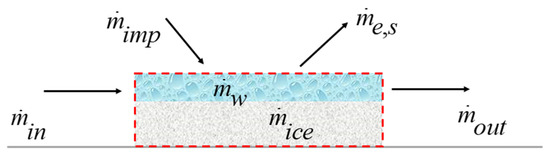
Figure 6.
Mass balance diagram based on the Messinger Model.
2.4.2. Energy Balance
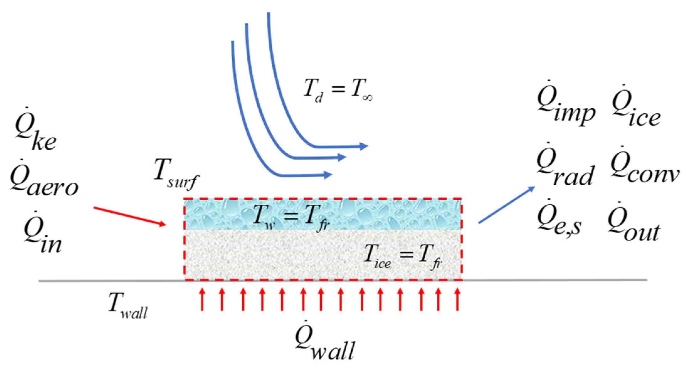
Figure 7 shows the 2D CV of a single cell of the icing thermodynamic model on the airfoil surface with the associated heat transfer terms acting on it. The cooling terms of the heat transfer energy balance include the impinging water droplets , radiation , evaporation or sublimation , runback out of the CV , icing , and convective heat transfer . The heating terms include kinetic heating , aerodynamic heating , runback into the CV , and the anti-icing heat flux at the wall of the airfoil . A complete derivation for each of these terms can be found in Appendix A. The steady-state energy balance is given by Equation (23):
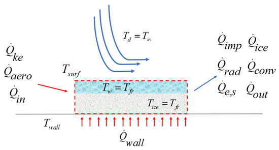
Figure 7.
Heat balance diagram based on the Messinger Model.
2.4.3. Stagnation Line Freezing Fraction
By re-arranging the energy balance of Equation (23), an expression for the freezing fraction ff can be found, as shown in Equation (24). The expression of the stagnation line freezing fraction ff0 reduces to Equation (25):
2.4.4. Possible Icing/Anti-Icing Scenarios
Four test cases could occur with the proposed arrangement of the heat and mass balances: (1) all of the water remains liquid (ff0 = 0 and Tsurf ≥ 0 °C); (2) only some of the water freezes (0 < ff0 < 1 and Tsurf = 0 °C); (3) all of the water freezes (ff0 = 1 and Tsurf < 0 °C); and (4) no water droplets are impinged, and the surface is dry.
When all the water remains liquid, the surface temperature is the one at the air–water interface. Also, no ice formation occurs; therefore, ff0 = 0 and Tsurf ≥ 0 °C. Both terms of the incoming mass flow and frozen ice mass are also zero (). Moreover, only water evaporation is accounted for since no ice is present in the system (). At the stagnation point, the energy balance reduces to Equation (26):
When a mixed water–ice layer is modeled, partial freezing of the incoming water occurs (0 < ff0 < 1). The surface temperature is the one at the air–water interface, and only the evaporation term is accounted for (no ice sublimation). The energy balance at the stagnation point is then given by Equation (27):
If the entirety of the water freezes, the surface temperature is the one at the air–ice interface. Total freezing indicates that ff0 = 1 and Tsurf < 0 °C. Both terms of the incoming and outgoing mass flows are also zero (). Moreover, only ice sublimation is accounted for since only ice is present in the system (). At the stagnation point, the energy balance reduces to Equation (28). Previous numerical and experimental works have shown that this case only occurs for small MVD values, low LWC values, and very low freestream temperatures (T∞< −20 °C) [25,30].
Finally, for the case of when no water impinges on the airfoil surface, the surface temperature is equal to that of the airfoil wall (Tsurf = Twall). Also, all mass and energy terms related to water or ice are zero. Therefore, Equation (23) reduces to Equation (29):
In this work, the assumption of a constant temperature in the water and ice layers dictate that cases 1 and 2 may only be modeled for a situation where the water or ice layers are at 0 °C (for liquid water right before freezing or for solid ice exactly at the freezing point). Case 3 may not be modeled with the proposed approach since the total freezing of the impacted droplets will likely occur at temperatures well below 0 °C. Case 4 can be modeled since no water or ice exist to begin with.
3. Results
3.1. Experimental and Numerical Model Setup
3.1.1. Experimental Rotor Tests
The test case consisted of a 0.66 m diameter 4-blade rotor with a NACA 4412 airfoil shape that operated under a range of rotor speeds of 3880 ≤ Ω ≤ 4950 RPM. The blades were twisted, and the chord varied from root to tip. The rotor was placed in AMIL’s 9 m ceiling cold chamber, replicating a hovering rotor operation. The icing spray was delivered through two nozzles positioned at the ceiling of the chamber, providing LWC = 6.3 g/m3 and MVD = 120 μm. Two air temperatures were used, T∞ = −5 °C and T∞ = −12 °C, to account for both the glaze and rime ice accretions. Photographs and measurements of the resulting ice shape for a wide range of rotor operational parameters have been reported in earlier publications [46]. Anti-icing tests for the same drone rotor were also conducted in the same cold chamber with a set of blades equipped with 0.1 mm thick heating elements having a length of 12 inches (0.3048 m) that were used to cover the LE of the blade from root to tip. The elements were 2″ wide (0.0508 m) and they covered an area of 1 inch downstream of the nose of the LE on both the upper and lower surfaces of the blades. More details on these tests can be found in [47].
3.1.2. UVLM Runs
The test case was run using the UVLM for 18 revolutions for ΔΨ = 10° using 10 × 25 vortex panels on each blade, and the first two rotor revolutions were used to slow-start the rotor. The presented UVLM data are the ones averaged over the last two simulated revolutions, where the calculations stabilize and do not change between timesteps.
3.2. Rotor Aerodynamic Modeling: From Comparison to Experiments
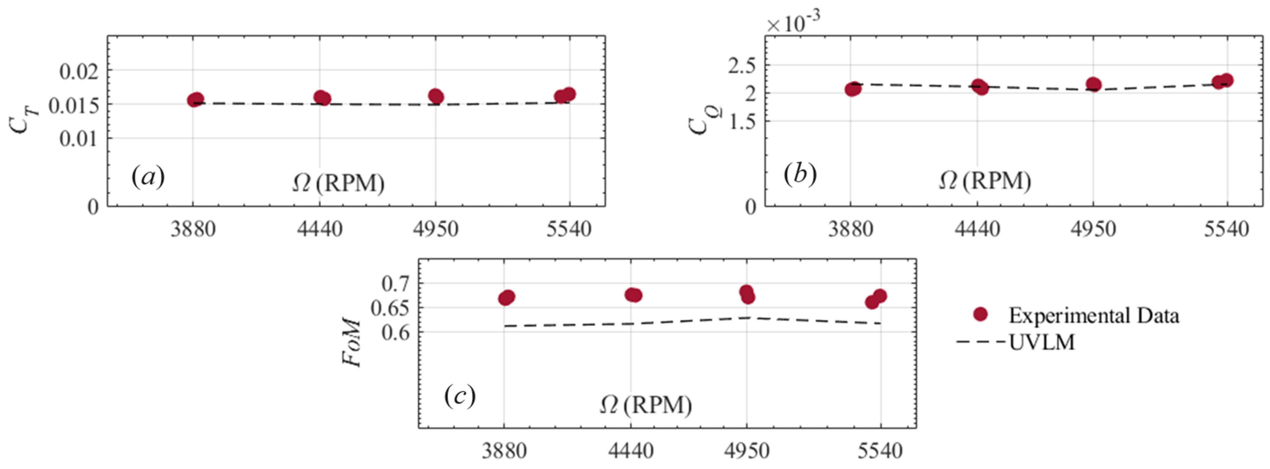
Figure 8 shows the variation in the hovering rotor aerodynamic parameters obtained from the experiments versus the numerical results for the (a) thrust coefficient CT; (b) torque coefficient CQ; and (c) Figure of Merit FoM. The agreement between the sets of data is within 10% for all simulated rotor speeds (Ω = 3880, 4440, 4950, and 5540 RPM).
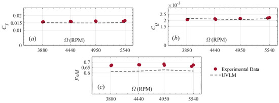
Figure 8.
Comparison between the numerical and experimental data for (a) CT; (b) CQ; and (c) FoM.
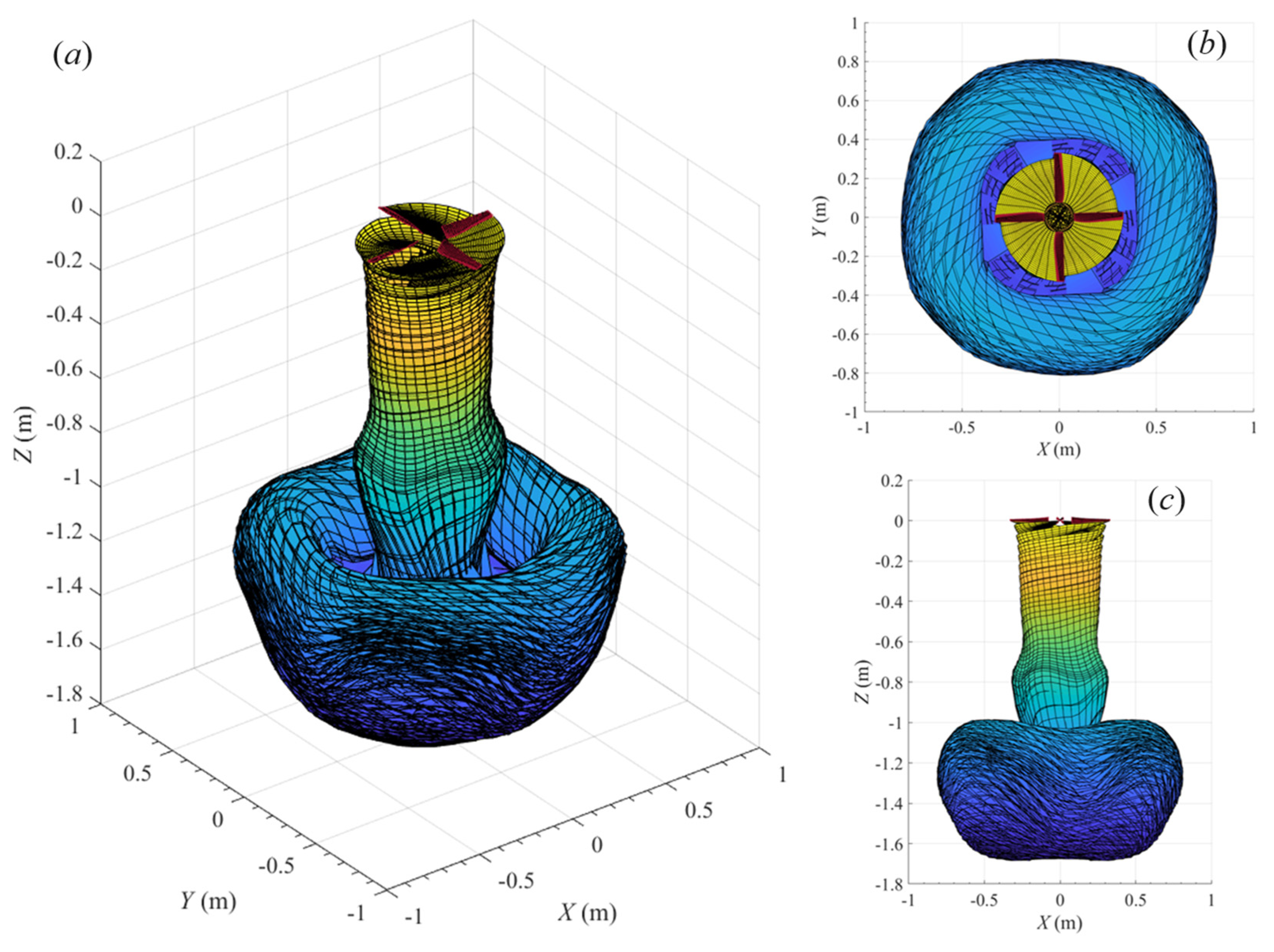
The hovering wake shape after 14 revolutions is also presented in Figure 9 for three view points: (a) parametric; (b) top; and (c) side. The wake shape and trajectory agree with the experimental observations and numerical predictions of previous studies [48]. The wake contracts below the rotor plane and is pushed underneath it as a result of the induced velocities and downwash of the rotating blades. The symmetric wake shape is obtained due to the absence of any axial or forward motion of the rotor, which makes the hovering rotation effect of the blade the sole driver of this symmetry. Finally, an inverted mushroom shape can be seen forming at 1 to 1.6 m below the rotor plane due to the weakening of the induced velocities and downwash, making the furthest away wake elements expand, create edge vortices, and rotate around themselves.
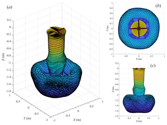
Figure 9.
Hovering wake shape obtained for Ω = 4950 RPM: (a) parametric view; (b) top view; and (c) side view.
Finally, when experimental thrust and torque measurements were compared between a ground clearance of 2 and 4 m (h/R = 6 and 12, respectively) in a previous publication [46], an average variation of around 3% between the two ground clearances was found for either aerodynamic parameter. As predicted in Figure 9, the expanding wake shape dissipates at around 1.8 m, making its influence on rotor performance weaker. Therefore, the UVLM predicts that no important effects should impact performance when ground clearances of 2 or 4 m are used, a phenomenon that was experimentally proven earlier [46]. Keeping in mind that higher rotation speeds produce a stronger downwash and are associated with axially farther, more expanding wake shapes, lower rotation speeds will therefore produce shorter wake shapes, and the effect of ground clearance on the tested rotor remains unchanged than that seen at 4950 RPM in Figure 8.
3.3. Rotor Icing Analysis: From Comparison to Experiments
3.3.1. Tests at T∞ = −5 °C
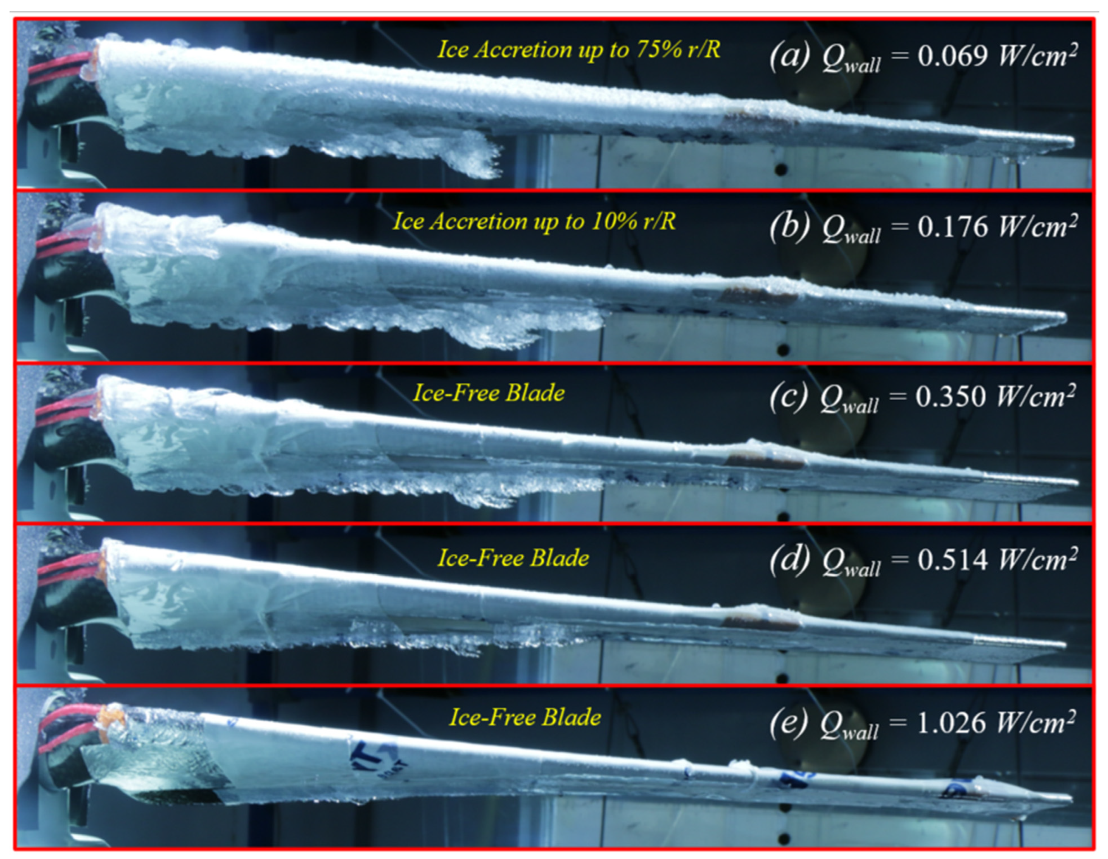
The experimental ice shape photographs of the tested drone with the heated rotor are shown in Figure 10 for the tests conducted at Ω = 3880 RPM and T∞ = −5 °C. As indicated in subfigures (a) to (e), each subfigure represents a photograph of a blade after a test is performed at a different heating power. The purpose of these tests was to determine the power required to eliminate ice formation on the rotor blades. Upon further examination, it was noticed that ice accretion on the LE only occurred for the two lowest tested heating powers = 0.069 and 0.176 W/cm2, with ice accretion happening between 0 and 75% of the blade radius for the former and up to only 10% of the radius for the latter. The LE was ice free for all higher values. Moreover, for the cases where ice was still found on the LE for lower heating powers, the ice was thicker near the root and became thinner towards the blade tip, where no ice was found even for the lowest tested .

Figure 10.
Experimental ice shapes on a blade for a case when Ω = 3880 RPM; LWC = 6.3 g/m3; MVD = 120 μm; and T∞ = −5 °C for test cases at = (a) 0.069; (b) 0.176; (c) 0.35; (d) 0.514; and (e) 1.026 W/cm2.
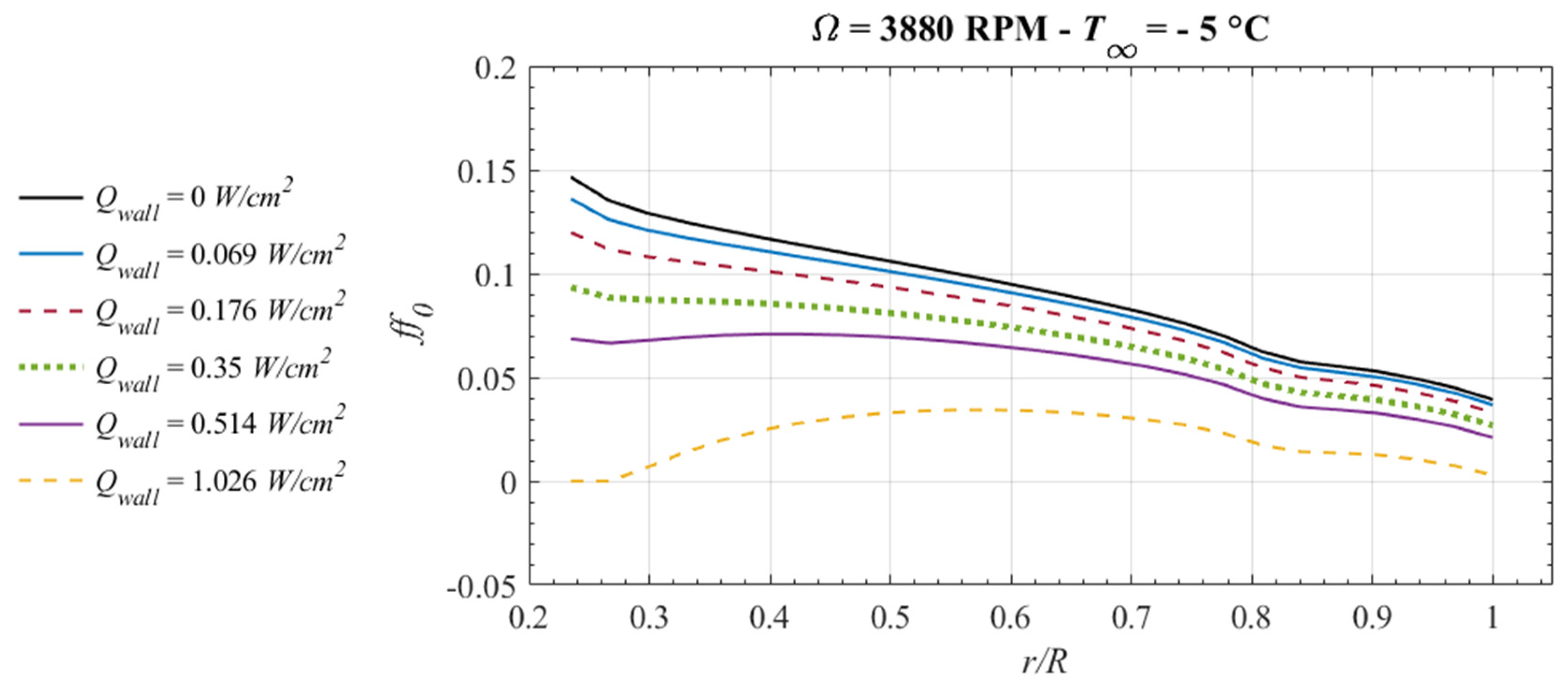
The test cases in Figure 10 were replicated using the proposed approach of the UVLM-RTH. Six test cases were ran using different values, corresponding to the ones conducted experimentally, plus one more case with = 0. The predicted ff0 using the numerical approach for each run is presented in Figure 11.
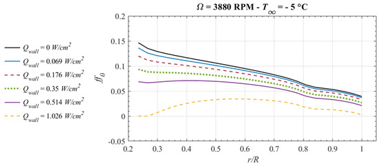
Figure 11.
UVLM predictions of the stagnation line freezing fraction ff0 for a case when Ω = 3880 RPM; LWC = 6.3 g/m3; MVD = 120 μm; and T∞ = −5 °C for test cases at = 0, 0.069; 0.176; 0.35; 0.514; and 1.026 W/cm2.
When no wall heating is modeled, the results show freezing fraction values that vary from 15% at the root of the blade down to less than 5% at the tip. When heating values are used, ff0 trends stay consistent, indicating that the thickest ice accretion will occur near the hub and becomes thinner going towards the tip, in agreement with the experimental ice shape seen earlier. Near the hub, low local blade velocities produce low convective heat transfer values that are easily overcome by the incoming heat from the wall. Near the tips, aerodynamic heating is significantly increased, and when combined with the incoming heat from the wall, the total heating energy terms become larger than all other cooling terms that the blade LE experiences.
As was increased, ff0 values decreased consistently throughout the blade span until zero values were predicted near the hub and root only when the modeled heating power was 1.026 W/cm2, which was higher than the experimentally required value of 0.35 W/cm2. However, at that value, the UVLM-RHT predictions show that only about 9% to 4% of the incoming water droplets will freeze, which could indicate that the discrepancy is either due to numerical errors or to a physical phenomenon not modeled numerically, such as ice shedding due to centrifugal forces.
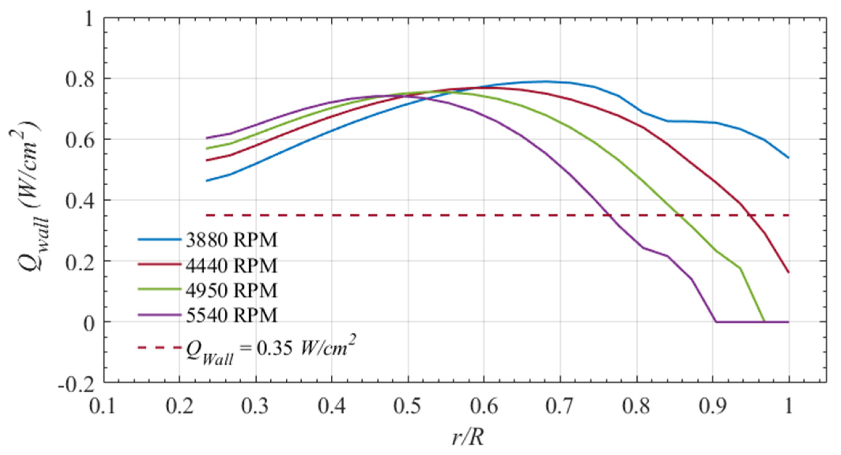
When the approach towards numerical modeling using the UVLM-RHT was changed, the required to prevent any water from freezing (maintain ff0 = 0) throughout the blade was calculated. The results are shown in Figure 12 for four test cases ran at −5 °C as well as 3880, 4440, 4950, and 5540 RPM. A point of reference was seen to occur at around the mid-span of the blade, where the predicted was the same for all rotor speeds. For smaller r/R values, the UVLM predicted a higher value for a higher Ω, whereas the inverse was true for r/R > 0.5. Cooling energy terms mostly dominated the first half of the blade and were enhanced by the increase in convective heat transfer due to the increase in rotation speed. However, aerodynamic heating overcame the cooling effects for the other blade-half, and the heating requirement significantly dropped as Ω was increased. Aerodynamic heating increased with a quadratic relationship with the local blade velocity, while all other cooling heat fluxes only increased linearly with the local air speed.
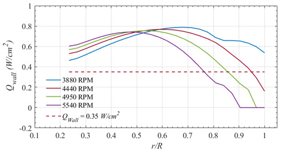
Figure 12.
UVLM predictions of the required anti-icing heat flux for a case when LWC = 6.3 g/m3; MVD = 120 μm; and T∞ = −5 °C for the test cases at 3880; 4440; 4950; and 5540 RPM.
To quantify the discrepancy between the UVLM-RHT predictions and experimental results, the numerical results were also compared with the maximum heating power that was experimentally determined to be sufficient to prevent any ice accumulation on the blades. In these experiments, a constant heat flux of = 0.35 W/cm2 was applied throughout the blade, while the UVLM predictions assumed a constant blade wall temperature and a radially variable . Nevertheless, the numerical results overestimate the required by as much as 50% in the central region of the blade (0.3 < r/R < 0.9, depending on Ω).
The experimental ice shapes for the test cases of Figure 12 with the same icing conditions are shown in Figure 13 for Ω = 3880, 4440, and 4950 RPM. The bulk of the ice thickness was found near the mid-span of the blade and seemed to shift closer to the hub as the rotor speed was increased, an effect directly reflected in the numerical results of Figure 12. More importantly, there was an absence of ice accretion near the tips for the test case at 4950 RPM, while both tests at the lower speeds showed a pertinent level of ice accumulation in the same region. This confirms the calculations of the UVLM-RHT, where aerodynamic heating was determined to be high enough to reduce the freezing fraction of water near the tips.
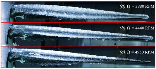
Figure 13.
Experimental ice shapes on blades for the tests at LWC = 6.3 g/m3; MVD = 120 μm and T∞ = −5 °C and at (a) 3880 RPM; (b) 4440 RPM; and (c) 4950 RPM.
3.3.2. Tests at T∞ = −12 °C
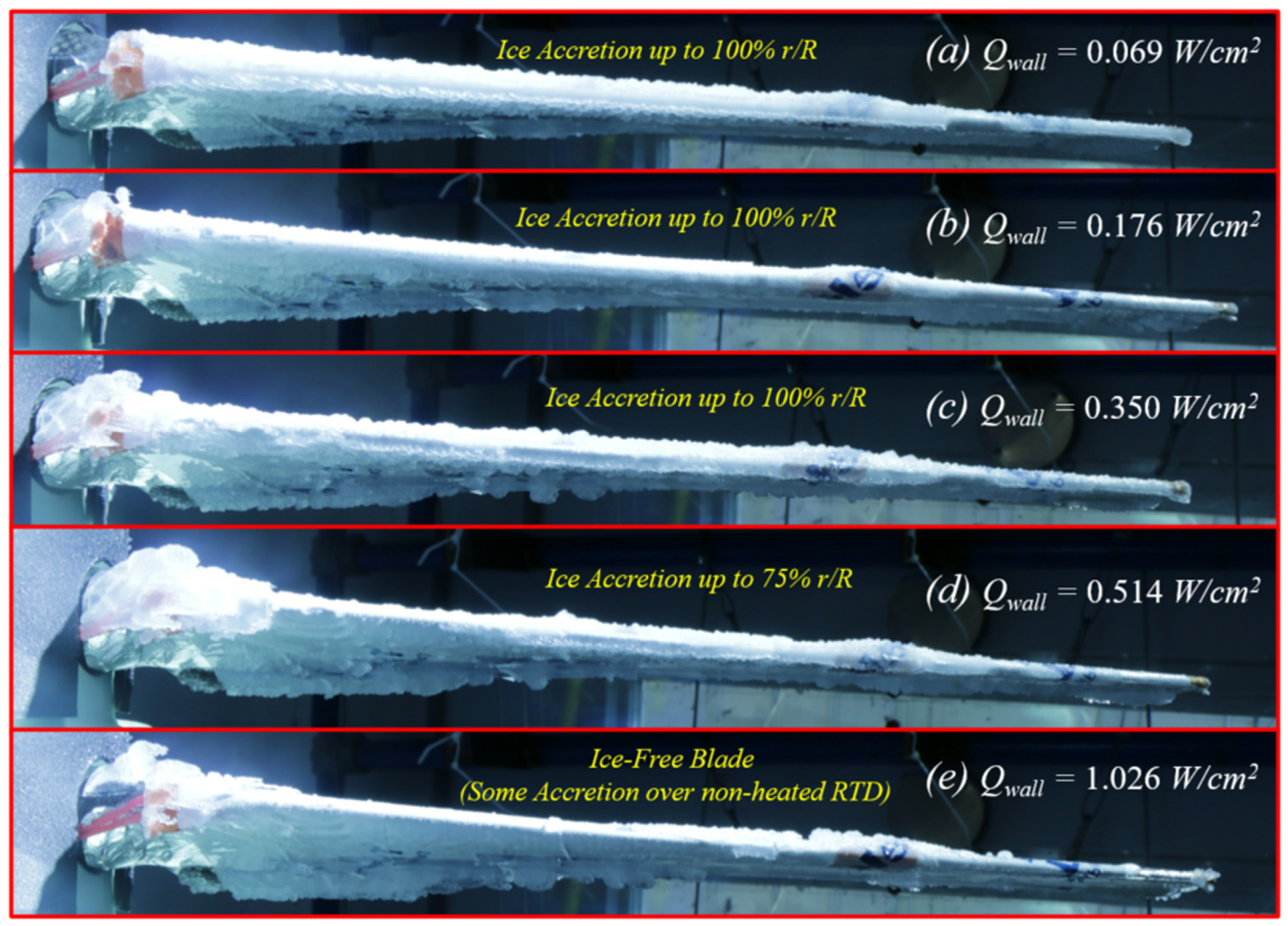
Another set of tests on the same heated rotor was carried out at Ω = 3880 RPM and T∞ = −12 °C. Similar heating powers were applied as the ones used earlier for the tests at a higher air temperature. The results of the experimental ice shapes for the tests at the colder temperature are presented in Figure 14a–e. For these tests, ice accretion was found even when a lot of heating power was used. Examining the photographs shows that in fact, ice formed on the LE across the whole span of the blade, even near the tips, and even when a heating power of = 0.514 W/cm2 was applied. What is also common with the ice shapes seen at T∞ = −5 °C (Figure 10) is that the ice tended to be thicker near the hub and thinner going towards the tip. Compared to the tests conducted at −5 °C, the higher temperature difference significantly increases the cooling brought by convective heat transfer, and the latent heat of fusion of the colder droplets also becomes significantly more important. Since the positive energy terms brought by aerodynamic heating and the heating elements did not change, the energy balance turns towards freezing of the incoming droplets and thus showing thicker ice accretions. It is also worthy to note that the ice seen in Figure 14 is more opaque compared to that of Figure 10, indicating a mixed glaze–rime ice type due to more droplets freezing faster upon impact.

Figure 14.
Experimental ice shapes on the blades for a case when Ω = 3880 RPM; LWC = 6.3 g/m3; MVD = 120 μm; and T∞ = −12 °C for the test cases at = (a) 0.069; (b) 0.176; (c) 0.35; (d) 0.514; and (e) 1.026 W/cm2.
However, when the maximum heating power of the system ( = 1.026 W/cm2) was used, Figure 14e shows no ice formation on the LE, except for a region above an installed RTD that prevented heating from the heating elements. Nonetheless, it was determined that a minimum of 1.026 W/cm2 was required to fully protect the blades, had the RTD not been installed.
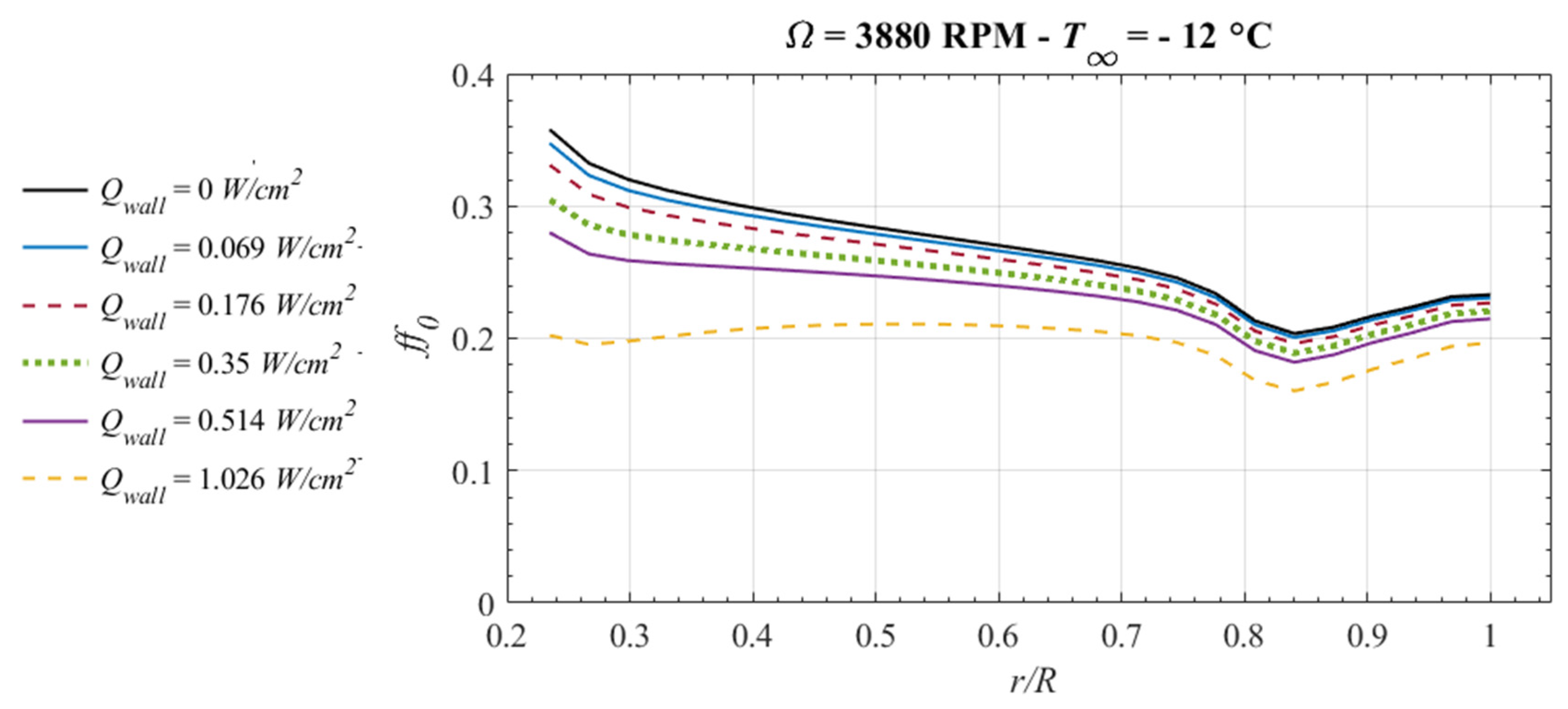
Replicated test cases of Figure 14 were carried out for the different values using the UVLM-RHT, and the results of the predicted ff0 values are presented in Figure 15. One thing to note is that the freezing fractions predicted are almost double those for the test cases at the higher air temperature presented earlier, which means thicker ice accretions across the blade span. The ff0 curves were decreasing from the hub to around 85% of the radius. A notable difference compared to the tests at T∞ = −5 °C, however, is the trend’s reversal at this region, where the ff0 values start increasing when heading towards the tips. Upon the examination of calculations, it was found that the three-dimensional rotor tip effects were responsible for this increase. The convective heat transfer remarkably increased in that region and was amplified by the larger temperature gradient for the tests at T∞ = −12 °C compared to those at T∞ = −5 °C. The numerical analyses show that none of the simulated heating powers prevent ice accretion, with the highest predicting ff0 ≈ 0.2 values from hub to tip, showing an obvious disagreement between the UVLM-RHT predictions and the experimental data.
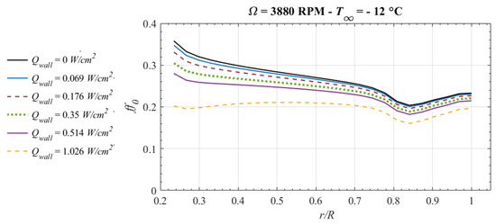
Figure 15.
UVLM predictions of the stagnation line freezing fraction ff0 for a case when Ω = 3880 RPM; LWC = 6.3 g/m3; MVD = 120 μm; and T∞ = −12 °C for the test cases at = 0, 0.069; 0.176; 0.35; 0.514; and 1.026 W/cm2.
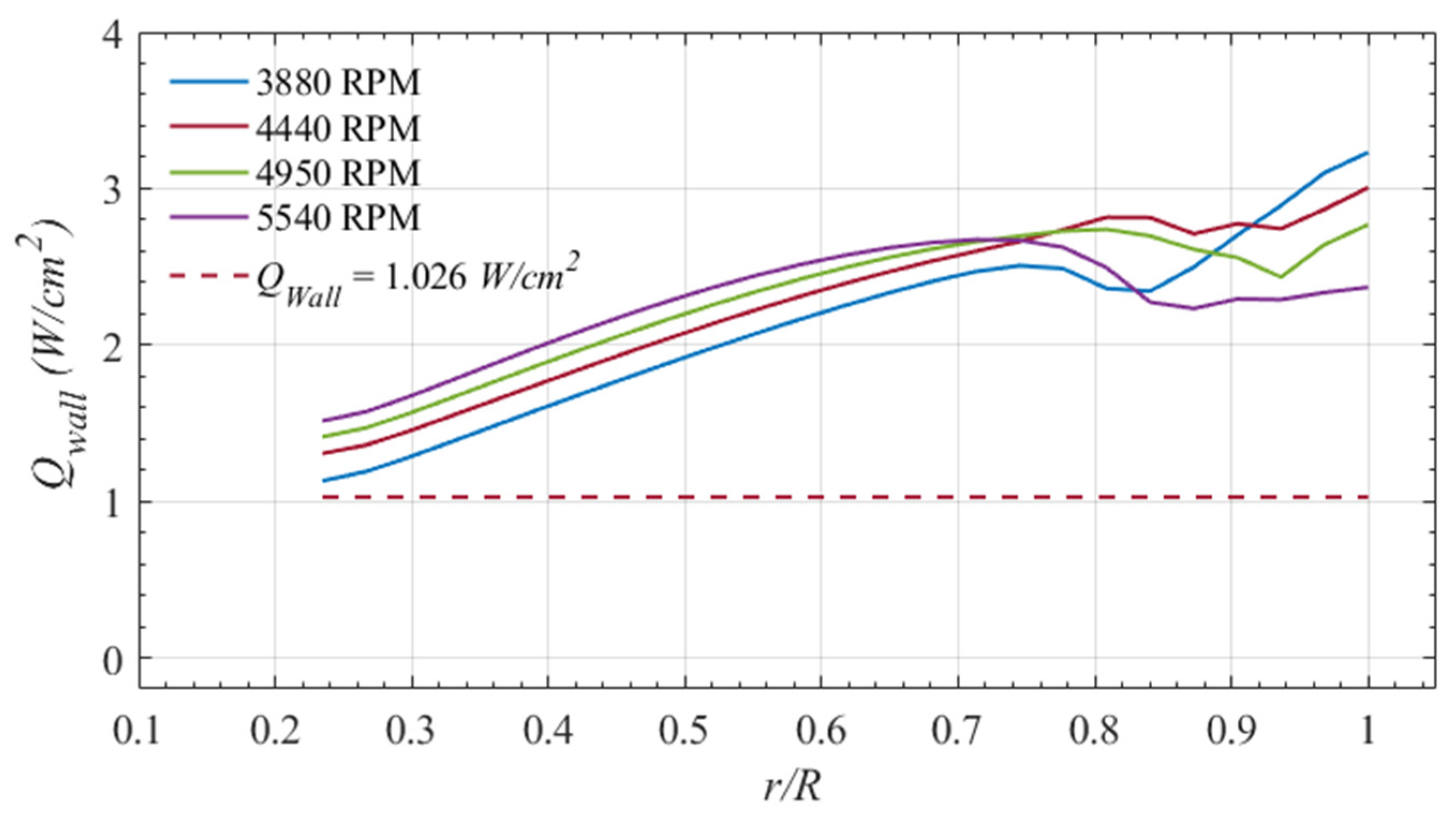
The heating power required to prevent ice accretion (ff0 = 0) throughout the blade, predicted by the UVLM-RHT, is presented in Figure 16 for the four test cases that were ran at −12 °C as well as 3880, 4440, 4950, and 5540 RPM. The predicted values almost continuously increase from hub to tip, with a slight disruption to its value near 80% of the span. For the tests at this lower temperature, the cooling effects from the energy balance therefore overcame all the heating terms, and unlike the test conducted at −5 °C, it is predicted that important heat inputs from the IPS are required to protect the tips from ice accumulation.
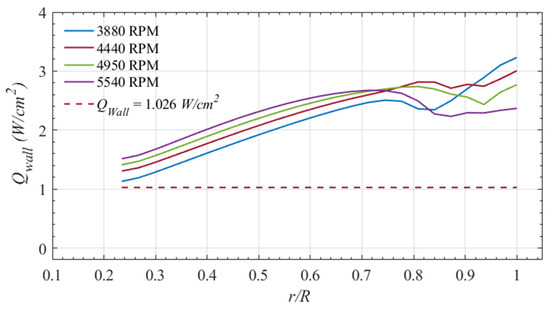
Figure 16.
UVLM predictions of the required anti-icing heat flux for a case when LWC = 6.3 g/m3; MVD = 120 μm; and T∞ = −12 °C for the test cases at 3880; 4440; 4950; and 5540 RPM.
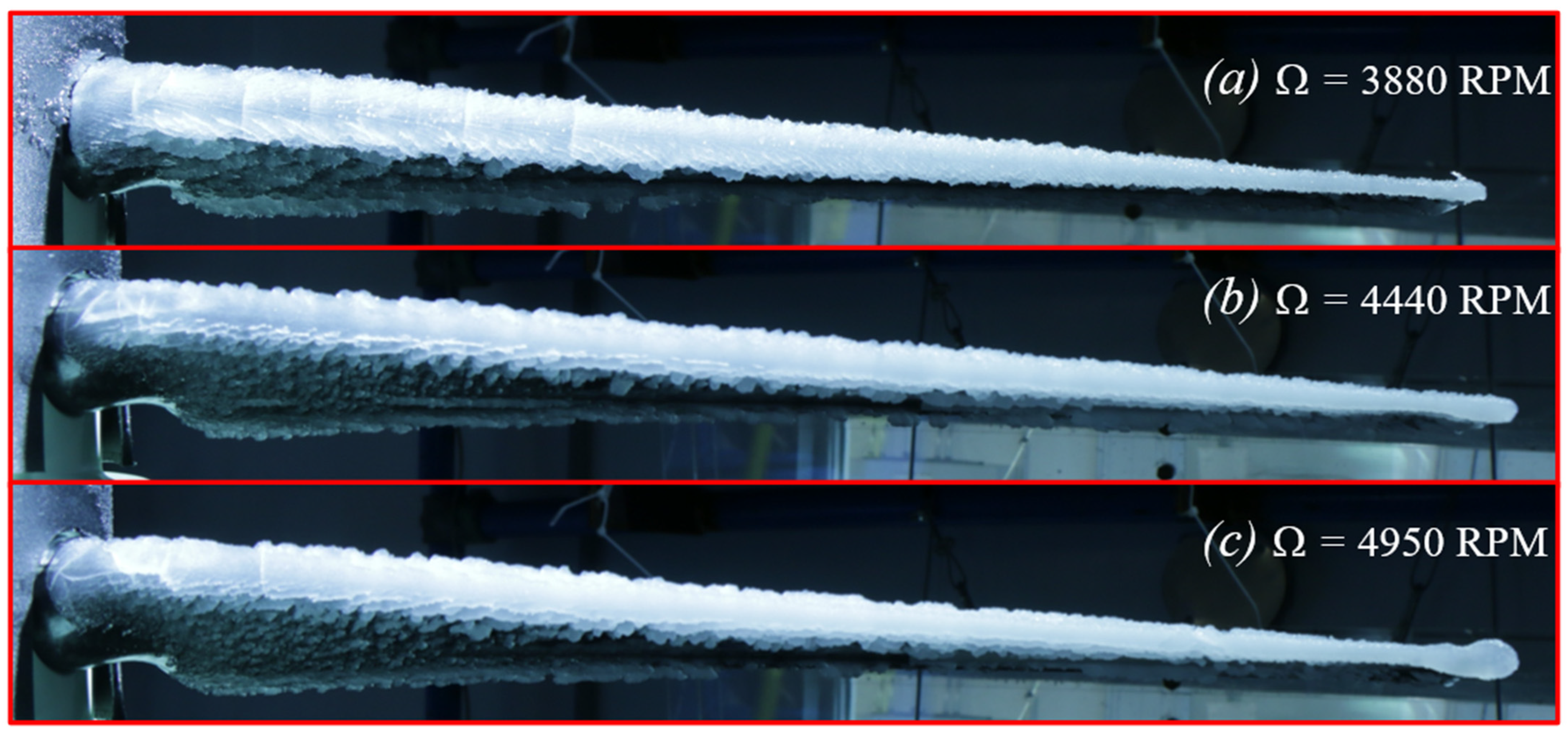
The experimental ice shapes that were obtained at different rotor speeds and at −12 °C confirm this finding (Figure 17), where ice accretion is found throughout the blade span, even near the tips, and the highest rotor speed. Finally, the discrepancy between the numerically and experimentally required anti-icing heat flux for ice prevention was higher at −12 °C. Compared to the maximum determined value = 1.026 W/cm2, the UVLM-RHT shows a discrepancy of around 50% at the hub and predicts a value almost triple of what was observed experimentally near the tips.
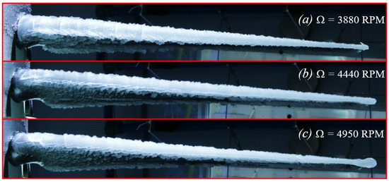
Figure 17.
Experimental ice shapes on the blades for the tests at LWC = 6.3 g/m3; MVD = 120 μm; and T∞ = −12 °C and at (a) 3880 RPM; (b) 4440 RPM; and (c) 4950 RPM.
4. Discussion
The preliminary approach for rotor icing modeling developed in this paper shows that the predicted ice shape locations and variation agree qualitatively with the experimental data. Moreover, the effects brought by the air temperature and rotor speed on the overall cooling and heating terms of the energy balance are well reflected and capture some aspects of the icing process on the rotors. However, the presented results show that the model still suffers from relatively high prediction inaccuracies and could not yet be considered reliable for full-on rotor icing modeling.
One thing to note about the experimental setup presented earlier is the use of relatively high values of LWC (6.31 g/m3) and MVD (120 μm) that are thought to be a major source for the discrepancies seen earlier, especially since the simplified icing model neglects temperature changes in the water and ice layers [27]. High LWC values correspond to thicker water layers with a variable temperature on top of the airfoil surface, which would directly affect the freezing process as well as the convective heat transfer. Moreover, droplets larger than 50 μm may experience splashing upon impact and end up not flowing over the rotor [45].
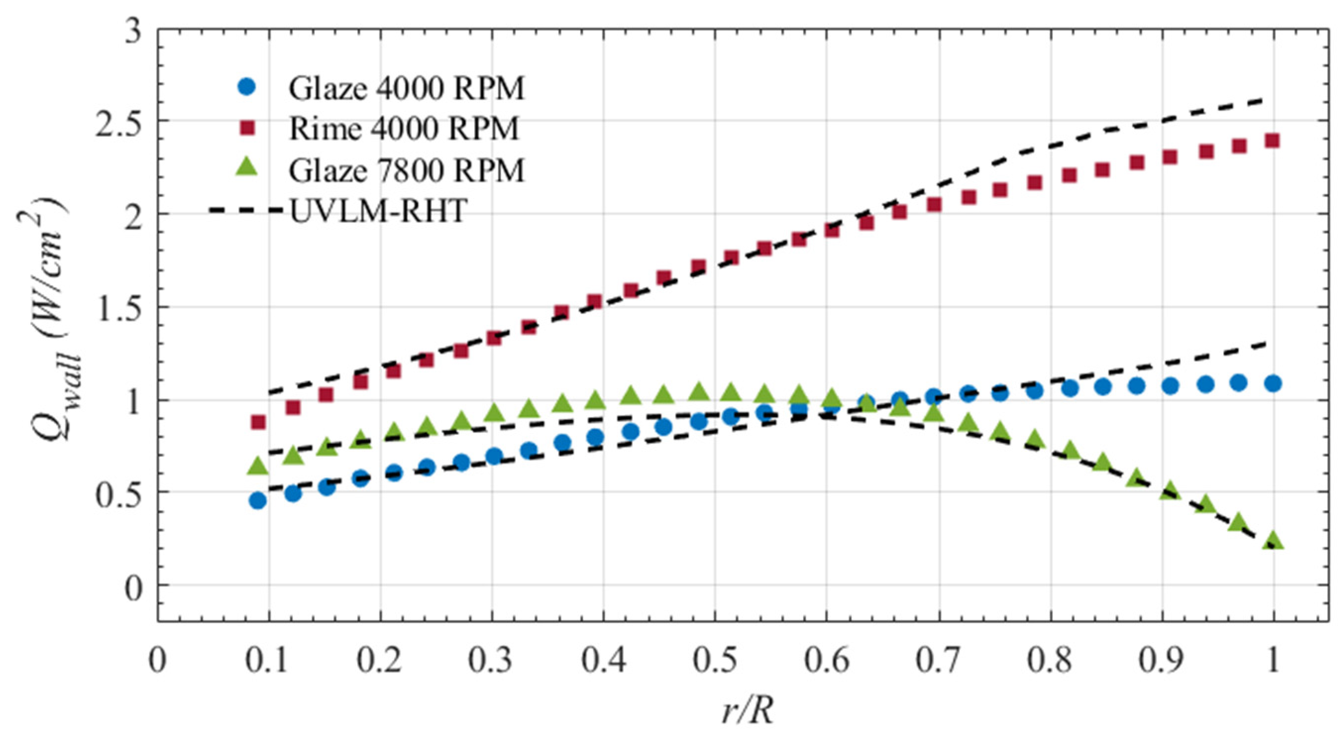
The UVLM-RHT method was used to analyze another rotor test case with a heat-leading edge from the literature [49]. The test case consisted of a 0.33 m diameter 2-blade rotor with an operation at either 4000 or 7800 RPM. The icing conditions were LWC = 0.78 g/m3 and MVD = 20 μm, and two air temperatures were used, T∞ = −5 °C and T∞ = −10 °C. The authors of that work developed and validated with experimental data their own simplified numerical methodology to calculate the required anti-icing heat flux for three test cases, as presented in Figure 18. The results obtained from the UVLM-RHT method for similar icing and operation conditions are also plotted and compared.
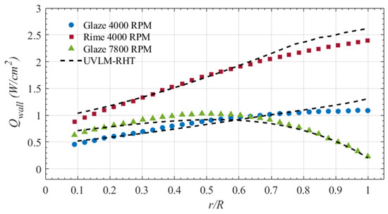
Figure 18.
Comparison between the predicted by the UVLM-RHT method and numerical data from the literature [49].
The results of Figure 18 show that the UVLM-RHT predictions agree well with those of the literature for all three presented test cases. For the glaze and rime ice test cases at the lower speed, the predictions of both numerical approaches are almost the same, except near the tip regions where the UVLM-RHT predicts 15% higher values. For the glaze ice test case at 7800 RPM, the predictions match from hub to tip, and the effects of aerodynamic heating are captured by both numerical tools. Keeping in mind that the results of [49] were also validated using their experimental data, it can be concluded that the UVLM-RHT method predicts acceptable estimates of the for lower LWC and MVD icing conditions.
5. Conclusions
This paper presented a preliminary and novel approach towards modeling rotor icing using the Unsteady Vortex Lattice Method. This study expands upon a previously developed UVLM implementation for 3D rotor aerodynamic modeling by integrating a simplified steady-state icing thermodynamic model along the stagnation line of the blade. A viscous coupling algorithm, employing a modified α method, integrates viscous data into the original inviscid calculations of the UVLM. This algorithm is subsequently utilized to compute convective heat transfer levels for each r/R through a CFD-based correlation for airfoils. The collection efficiency at the stagnation line is determined using Langmuir and Blodgett’s correlation, and a simplified steady-state icing model is used by solving the mass and energy balance equations. Given the preliminary nature of the icing approach, the analysis is focused on the stagnation line freezing fraction as well as the wall anti-icing heat flux.
The results are focused on simulating a previous experimental setup of a 4-blade rotor fitted with heated blades via electro-thermal heating elements. The aerodynamic performance of the rotor is captured well by the UVLM, within 10% of the measured thrust and torque coefficients, and the predicted wake shape agrees well with our experiments. For the icing analysis at −5°C, the suggested method tends to overestimate the necessary anti-icing flux by approximately 50%, despite accurately forecasting the impact of aerodynamic heating on the prevention of ice formation near the blade tips. At −12 °C, the visualizations of ice formation at various anti-icing heating powers align closely with the UVLM’s predictions. However, a notable disparity arises when attempting to predict the essential heat load for eliminating any ice formation.
The large discrepancy obtained was thought to be due to the use of large LWC and MVD values in the experiment, which may have exaggerated the discrepancy produced by the simplified icing model of this work. By simulating another rotor test case from the literature with much lower LWC and MVD values, the results showed excellent predictions of required anti-icing heat flux that agree within 10% of the numerical and experimental predictions of the literature.
Further work is required to develop the proposed method into a more accurate tool for rotor icing analyses. Mainly, a model for water and ice film thicknesses and temperatures will be implemented. Furthermore, a model for ice-induced roughness will be incorporated to better adapt the tool for ice shape predictions. Roughness effects arising from ice accretion are known to enhance convective heat transfer and correlate directly with the ice shape produced. For now, this tool is treated as a first step towards a low-cost simplified tool to predict icing and the required running wet anti-icing heat flux with significant ice accumulation allowed.
Author Contributions
Conceptualization, A.S.; methodology, A.S.; software, A.S. and F.M.; validation, A.S., F.M. and E.V.; formal analysis, A.S. and E.V.; investigation, A.S.; resources, A.S., F.M. and E.V.; data curation, A.S. and E.V.; writing—original draft preparation, A.S.; writing—review and editing, A.S.; visualization, A.S., F.M. and E.V.; supervision, A.S. and F.M.; project administration, A.S.; funding acquisition, M.B. and M.L. All authors have read and agreed to the published version of the manuscript.
Funding
This research was funded by Bell Textron Canada Ltd.
Data Availability Statement
The data used in this work are confidential.
Acknowledgments
The authors acknowledge the support provided by Bell Textron Canada Ltd.
Conflicts of Interest
The authors declare no conflicts of interest.
Appendix A
- Mass Transfer Equations
The mass flow components of Equation (22) are defined as follows:
- (1)
- is the mass flow rate from the incoming droplets of water (carried by the freestream):
- (2)
- is the mass flow rate moving from a neighboring cell into the CV. In this analysis, only the stagnation point is considered, so the only term for the incoming mass flow rate into the CV is the one from the impinging droplets and .
- (3)
- is one of the two quantities describing the evaporating mass flow rate () or the sublimating mass flow rate (). In this work, only is accounted for in the case of a glaze ice accretion (Equation (31)), whereas only is accounted for in the case of a rime ice accretion (Equation (32)). is the saturation vapor pressure of air over water given by Equation (33) (T > 0 °C), and is the saturation vapor pressure of air over ice given by Equation (34) (T ≤ 0 °C). Both equations are obtained from [50].
hG is the gas-phase convective mass transfer coefficient (Equation (35)); hc is the convective heat transfer coefficient; and Pra and Sca are the air Prandtl number and Schmidt numbers, respectively. Both are evaluated at the film temperature Tfilm, where μa, ρa, cp,a, and DV are the air-specific kinematic viscosity, density, specific heat constant, and the diffusivity of water vapor in air, respectively, expressed by Equation (36) in m2/s [51].
- (4)
- is the amount of ice that is frozen on the surface. This term can be calculated by knowing the value of the freezing fraction ff. The latter is defined as the ratio of the amount of frozen water onto the surface to the total amount of water flow into the CV, as described by Equation (37). By rearranging the terms, and remembering that this analysis only deals with the stagnation point (), the frozen amount of ice can be calculated by Equation (38):
- (5)
- is the mass flow rate going out of the CV into the neighboring cell, which is also equal to the amount of unfrozen water in the cell. Since all other mass flow terms are accounted for by their own correlations, it is the only remaining unknown term in the mass balance (Equation (22)) and can be calculated by Equation (39):
- Energy Transfer Equations
- (1)
- is the heat lost from the CV by convective heat transfer (Equation (40)). In this work, this energy term is accounted for by first calculating the Nu through the coupled UVLM-RHT approach proposed in this paper. Correlations (15) or (16) are proposed as a means to calculating the Nu at the stagnation point of the airfoil (NACA 0012 or NACA 4412, respectively), which is, in turn, used in Equation (12) to calculate the heat transfer coefficient hc.
- (2)
- is the heat lost from the CV to raise the temperature of the impinging water droplets from the freestream temperature T∞ to the freezing temperature of water Tfr = 0 °C (Equation (41)):
- (3)
- is the heat lost from the CV due to icing (Equation (42)). It consists of two terms: the first is the heat capacity of ice when increasing its temperature from the surface temperature to the freezing temperature. The other term represents the energy released by the phase change of water to ice (which occurs at a constant temperature) and is referred to as the latent heat of fusion. For the analysis in this paper, the temperature is assumed to be constant within the water and ice layers; therefore, Tsurf = Tfr = 0 °C, and the first term of Equation (42) disappears:
- (4)
- is the heat lost from the CV by water flowing out and into the neighboring CV (Equation (43)). For the analysis in this paper, the temperature is assumed to be constant within the water and ice layers; therefore, Tsurf = Tfr = 0°C and = 0.
- (5)
- is the heat lost from the CV due to radiation (Equation (44)). σ = 5.6703 × 10⁻⁸ (W/m2.K4) is the Stefan–Boltzmann constant, and υ is the emissivity level at the water–air or ice–air interface (assumed constant at υ = 0.9).
- (6)
- is the heat lost from the CV due to the evaporation of water (Equation (45)) [28,52]. is the evaporation function given by Equation (46); e0 =27.03 is the saturation vapor pressure constant; and is the evaporation parameter given by Equation (47) [53]. is used for airflow over water, when only a liquid water film flows over the airfoil (ff0 = 0 and Tsurf > 0°C) or when a water–ice mix is predicted (0 < ff0 < 1 and Tsurf = 0 °C), and the surface represents an air–water interface.
- (7)
- is the heat lost from the surface due to the sublimation of ice (Equation (48)) [28,52]. is the sublimation parameter given by Equation (49). is used for the airflow over ice, when ff0 = 1 and Tsurf < 0 °C, and the surface represents an air–ice interface.
- (8)
- is the heat gained by the CV from the kinetic energy of the water droplets striking the surface (Equation (50)):
- (9)
- is the heat gained by the CV due to aerodynamic heating (Equation (51)), where TT is the total air temperature. is the adiabatic recovery factor (either or depending on whether the flow conditions are laminar or turbulent, respectively [54]). In this work, the complex flow generated by the blades and their wakes is assumed to provide turbulent flow conditions.
- (10)
- is the heat gained by the CV by water flowing into it from a neighboring CV. For the analysis at the stagnation point, the only incoming water is from the impinging droplets; therefore, .
- (11)
- is the sought-after heat flux required to anti-ice the blade surface, which was given previously by Equation (23).
Appendix B. Air, Water and Ice-Specific Properties

Table A1.
Air-specific properties.
Table A1.
Air-specific properties.
| Symbol | Definition | Value | Unit |
|---|---|---|---|
| Cp,a | Specific heat capacity of air | 1005 | J/kg.K |
| Cp,w | Specific heat capacity of liquid water | 4184 | J/kg.K |
| Cp,i | Specific heat capacity of ice | 2108 | J/kg.K |
| Lf | Latent heat of fusion of water | 334 × 103 | J/kg |
| Le | Latent heat of water evaporation | 2257 × 103 | J/kg |
| Ls | Latent heat of sublimation of ice | 2838 × 103 | J/kg |
| ρa | Density of air | 1.316 | kg/m3 |
| ρw | Density of water | 997 | kg/m3 |
| ρi,g | Density of glaze ice | 917 | kg/m3 |
| ρi,r | Density of rime ice | 880 | kg/m3 |
| R | Molecular gas constant of air | 287 | J/kg.K |
| μa | Kinematic viscosity of air | 12.85 × 10⁻⁶ | m2/s |
| νa | Dynamic viscosity of air | 16.9 × 10⁻⁶ | kg/m.s |
| P∞ | Atmospheric pressure | 101,300 | Pa |
| ka | Thermal conductivity of air | 23.97 × 10⁻⁴ | m/W.K |
| Pra | Prandtl number of air | 0.7085 | - |
| Sca | Schmidt number of air | 0.4708 | - |
| Lea | Lewis number of air | 0.6645 | - |
| σ | Stefan–Boltzmann constant | 5.6703 × 10⁻⁸ | W/m2.K4 |
| υw | Emissivity of water | ≈1 | - |
References
- Cao, Y.; Tan, W.; Wu, Z. Aircraft icing: An ongoing threat to aviation safety. Aerosp. Sci. Technol. 2018, 75, 353–385. [Google Scholar] [CrossRef]
- Gao, M.; Hugenholtz, C.H.; Fox, T.A.; Kucharczyk, M.; Barchyn, T.E.; Nesbit, P.R. Weather constraints on global drone flyability. Sci. Rep. 2021, 11, 12092. [Google Scholar] [CrossRef] [PubMed]
- Hassanalian, M.; Abdelkefi, A. Classifications, applications, and design challenges of drones: A review. Prog. Aerosp. Sci. 2017, 91, 99–131. [Google Scholar] [CrossRef]
- Vergouw, B.; Nagel, H.; Bondt, G.; Custers, B. Drone technology: Types, payloads, applications, frequency spectrum issues and future developments. In The Future of Drone Use: Opportunities and Threats from Ethical and Legal Perspectives; T.M.C. Asser Press: The Hague, The Netherlands, 2016; pp. 21–45. [Google Scholar]
- Liu, Y.; Li, L.; Ning, Z.; Tian, W.; Hu, H. Experimental investigation on the dynamic icing process over a rotating propeller model. J. Propuls. Power 2018, 34, 933–946. [Google Scholar] [CrossRef]
- Villeneuve, E.; Samad, A.; Volat, C.; Beland, M.; Lapalme, M. Experimental Assessment of the Ice Protection Effectiveness of Icephobic Coatings for a Hovering Drone Rotor. Cold Reg. Sci. Technol. 2023, 210, 103858. [Google Scholar] [CrossRef]
- Han, N.; Hu, H.; Hu, H. An Experimental Investigation to Assess the Effectiveness of Various Anti-Icing Coatings for UAV Propeller Icing Mitigation. In Proceedings of the AIAA Aviation 2022 Forum, Chicago, IL, USA, 27 June–1 July 2022. [Google Scholar] [CrossRef]
- Aubert, R. Additional Considerations for Analytical Modeling of Rotor Blade Ice. In Proceedings of the SAE 2015 International Conference on Icing of Aircraft, Engines, and Structures, Prague, Czech Republic, 22–25 June 2015; Available online: https://saemobilus.sae.org/content/2015-01-2080 (accessed on 8 February 2024).
- Gent, R.W.; Moser, R.J.; Cansdale, J.T.; Dart, N.P. The Role of Analysis in the Development of Rotor Ice Protection Systems; SAE Technical Paper; SAE: Warrendale, PA, USA, 2003. [Google Scholar] [CrossRef]
- Wright, W. User Manual for LEWICE Ver. 3.2; NASA Glenn Research Center: Cleveland, OH, USA, 2008. Available online: https://ntrs.nasa.gov/search.jsp?R=20080048307 (accessed on 8 February 2024).
- Guffond, D.; Brunet, L. Validation du Programme Bidimensionnel de Capitation; Oce National D’Etudes et de Recherches Aerospatiales. ONERA RP 1988, 20, 5146. [Google Scholar]
- Beaugendre, H.; Morency, F.; Habashi, W.G. Development of a second generation in-flight icing simulation code. J. Fluids Eng. 2006, 128, 378–387. [Google Scholar] [CrossRef]
- Morency, F.; Tezok, F.; Paraschivoiu, I. Anti-icing system simulation using CANICE. J. Aircr. 1999, 36, 999–1006. [Google Scholar] [CrossRef]
- The National Transportation Safety Board (NTSB). National Transportation Safety Board Aviation Accident Final Report; The National Transportation Safety Board (NTSB): Soldotna, AK, USA, 2005. [Google Scholar]
- Ghenai, C.; Lin, C.X. Verification and validation of NASA LEWICE 2.2 icing software code. J. Aircr. 2006, 43, 1253–1258. [Google Scholar] [CrossRef]
- Habashi, W.G.; Aubé, M.; Baruzzi, G.; Morency, F.; Tran, P.; Narramore, J.C. FENSAP-ICE: A fully-3d in-flight icing simulation system for aircraft, rotorcraft and UAVS. In Proceedings of the 24th International Congress of The Aeronautical Sciences, Yokohama, Japan, 29 August–3 September 2004; pp. 1–10. Available online: http://www.icas.org/ICAS_ARCHIVE/ICAS2004/PAPERS/608.PDF (accessed on 8 February 2024).
- Chen, X.; Zhao, Q.-J. Numerical simulations for ice accretion on rotors using new three-dimensional icing model. J. Aircr. 2017, 54, 1428–1442. [Google Scholar] [CrossRef]
- Morelli, M.; Guardone, A. A simulation framework for rotorcraft ice accretion and shedding. Aerosp. Sci. Technol. 2022, 129, 107157. [Google Scholar] [CrossRef]
- Lee, H.; Sengupta, B.; Araghizadeh, M.S.; Myong, R.S. Review of vortex methods for rotor aerodynamics and wake dynamics. Adv. Aerodyn. 2022, 4, 20. [Google Scholar] [CrossRef]
- Tugnoli, M.; Montagnani, D.; Syal, M.; Droandi, G.; Zanotti, A. Mid-fidelity approach to aerodynamic simulations of unconventional VTOL aircraft configurations. Aerosp. Sci. Technol. 2021, 115, 106804. [Google Scholar] [CrossRef]
- Joshi, H.; Thomas, P. Review of vortex lattice method for supersonic aircraft design. Aeronaut. J. 2023, 127, 1–35. [Google Scholar] [CrossRef]
- Samad, A.; Tagawa, G.B.S.; Morency, F.; Volat, C. Predicting rotor heat transfer using the viscous blade element momentum theory and unsteady vortex lattice method. Aerospace 2020, 7, 90. [Google Scholar] [CrossRef]
- Samad, A.; Tagawa, G.B.S.; Khamesi, R.R.; Morency, F.; Volat, C. Frossling Number Assessment for Airfoil Under Fully Turbulent Flow Conditions. J. Thermophys. Heat Trans. 2021, 36, 389–398. [Google Scholar] [CrossRef]
- Kim, J. Development of a Physics Based Methodology for the Prediction of Rotor Blade Ice Formation; SmarTech: Atlanta, GA, USA, 2015. [Google Scholar]
- Lavoie, P.; Pena, D.; Hoarau, Y.; Laurendeau, E. Comparison of thermodynamic models for ice accretion on airfoils. Int. J. Numer. Methods Heat Fluid Flow 2018, 28, 1004–1030. [Google Scholar] [CrossRef]
- Reid, T.; Baruzzi, G.S.; Habashi, W.G. FENSAP-ICE: Unsteady conjugate heat transfer simulation of electrothermal de-icing. J. Aircr. 2012, 49, 1101–1109. [Google Scholar] [CrossRef]
- Morency, F.; Tezok, F.; Paraschivoiu, I. Heat and mass transfer in the case of anti-icing system simulation. J. Aircr. 2000, 37, 245–252. [Google Scholar] [CrossRef]
- Özgen, S.; Canıbek, M. Ice accretion simulation on multi-element airfoils using extended Messinger model. J. Heat Mass Transf. 2009, 45, 305–322. [Google Scholar] [CrossRef]
- Messinger, B.L. Equilibrium temperature of an unheated icing surface as a function of air speed. J. Aeronaut. Sci. 1953, 20, 29–42. [Google Scholar] [CrossRef]
- Bond, T.H.; Anderson, D.N. Manual of Scaling Methods; NASA Glenn Research Center: Cleveland, OH, USA, 2004. Available online: https://ntrs.nasa.gov/citations/20040042486 (accessed on 8 February 2024).
- Poinsatte, P.; Newton, J.; De Witt, K.; Van Fossen, J. Heat transfer measurements from a smooth NACA 0012 airfoil. J Aircr 1991, 28, 892–898. [Google Scholar] [CrossRef]
- Katz, J.; Plotkin, A. Low Speed Aerodynamics, 2nd ed.; Cambridge University Press: New York, NY, USA, 2001; Volume 13. [Google Scholar]
- Leishman, J.G.; Bhagwat, M.J.; Bagai, A. Free-vortex filament methods for the analysis of helicopter rotor wakes. J. Aircr. 2002, 39, 759–775. [Google Scholar] [CrossRef]
- Proulx-Cabana, V.; Nguyen, M.T.; Prothin, S.; Michon, G.; Laurendeau, E. A Hybrid Non-Linear Unsteady Vortex Lattice-Vortex Particle Method for Rotor Blades Aerodynamic Simulations. Fluids 2022, 7, 81. [Google Scholar] [CrossRef]
- Bhagwat, M.J.; Leishman, J.G. Generalized viscous vortex model for application to free-vortex wake and aeroacoustic calculations. In Proceedings of the 58th Annual Forum Proceedings—American Helicopter Society, Montreal, QC, Canada, 11–13 June 2002; American Helicopter Society, Inc.: Montreal, QC, Canada, 2002; Volume 58, pp. 2042–2057. Available online: https://vtol.org/store/product/generalized-viscous-vortex-model-for-application-to-freevortex-wake-and-aeroacoustic-calculations-1996.cfm (accessed on 8 February 2024).
- Chung, K.H.; Kim, J.W.; Ryu, K.W.; Lee, K.T.; Lee, D.J. Sound generation and radiation from rotor tip-vortex pairing phenomenon. Am. Inst. Aeronaut. Astronaut. (AIAA) J. 2006, 44, 1181–1187. [Google Scholar] [CrossRef]
- Glauert, H. The effect of compressibility on the lift of an aerofoil. Proc. R. Soc. Lond. Ser. A Contain. Pap. A Math. Phys. Character 1928, 118, 113–119. [Google Scholar]
- Parenteau, M.; Plante, F.; Laurendeau, E.; Costes, M. Unsteady Coupling Algorithm for Lifting-Line Methods. In Proceedings of the 55th Aerospace Sciences Meeting, Grapevine, TX, USA, 9–13 January 2017; American Institute of Aeronautics and Astronautics AIAA: Grapevine, TX, USA, 2017; p. 951. [Google Scholar] [CrossRef]
- Gallay, S.; Laurendeau, E. Nonlinear generalized lifting-line coupling algorithms for pre/poststall flows. AIAA J. 2015, 53, 1784–1792. [Google Scholar] [CrossRef]
- Palacios, F.; Alonso, J.; Duraisamy, K.; Colonno, M.; Hicken, J.; Aranake, A.; Campos, A.; Copeland, S.; Economon, T.; Lonkar, A.; et al. Stanford University Unstructured (SU2): An open-source integrated computational environment for multi-physics simulation and design. In Proceedings of the 51st AIAA aerospace sciences meeting including the new horizons forum and aerospace exposition, Grapevine, TX, USA, 7–10 January 2013; p. 287. [Google Scholar] [CrossRef]
- Spalart, P.; Allmaras, S. A one-equation turbulence model for aerodynamic flows. In Proceedings of the 30th Aerospace Sciences Meeting and Exhibit, Reno, NV, USA, 6–9 January 1992; p. 439. [Google Scholar] [CrossRef]
- NASA Langley Turbulence Modeling Resources. Available online: https://turbmodels.larc.nasa.gov/ (accessed on 8 February 2024).
- Gregory, N.; O’Reilly, C.L. Low-Speed Aerodynamic Characteristics of NACA 0012 Aerofoil Section, Including the Effects of Upper-Surface Roughness Simulating Hoar Frost. 1970. Available online: https://reports.aerade.cranfield.ac.uk/handle/1826.2/3003 (accessed on 14 December 2023).
- Langmuir, I.; Blodgett, K. A Mathematical Investigation of Water Droplet Trajectories; Army Air Forces Technical Report No. 5418; Army Air Forces Headquarters, Air Technical Service Command: Wright-Patterson Air Force Base, OH, USA, 1946. [Google Scholar] [CrossRef]
- Palacios, J.L.; Han, Y.; Brouwers, E.W.; Smith, E.C. Icing environment rotor test stand liquid water content measurement procedures and ice shape correlation. J. Am. Helicopter Soc. 2012, 57, 29–40. [Google Scholar] [CrossRef]
- Villeneuve, E.; Samad, A.; Volat, C.; Beland, M.; Lapalme, M. An Experimental Apparatus for Icing Tests of Low Altitude Hovering Drones. Drones 2022, 6, 68. [Google Scholar] [CrossRef]
- Samad, A.; Villeneuve, E.; Volat, C.; Béland, M.; Lapalme, M. Experimental Assessment of the Ice Protection Effectiveness of Electrothermal Heating for a Hovering Drone Rotor. Exp. Therm. Fluid Sci. 2023, 149, 110992. [Google Scholar] [CrossRef]
- Caradonna, F. Performance measurement and wake characteristics of a model rotor in axial flight. J. Am. Helicopter Soc. 1999, 44, 101–108. [Google Scholar] [CrossRef]
- Karpen, N.; Diebald, S.; Dezitter, F.; Bonaccurso, E. Propeller-integrated airfoil heater system for small multirotor drones in icing environments: Anti-icing feasibility study. Cold Reg. Sci. Technol. 2022, 201, 103616. [Google Scholar] [CrossRef]
- Huang, J. A simple accurate formula for calculating saturation vapor pressure of water and ice. J. Appl. Meteorol. Climatol. 2018, 57, 1265–1272. [Google Scholar] [CrossRef]
- Pruppacher, H.R.; Klett, J.D.; Wang, P.K. Microphysics of clouds and precipitation. Aerosol Sci. Technol. 1998, 28, 381–382. [Google Scholar] [CrossRef]
- Myers, T.G. Extension to the Messinger model for aircraft icing. AIAA J. 2001, 39, 211–218. [Google Scholar] [CrossRef]
- Lowe, P.R. An approximating polynomial for the computation of saturation vapor pressure. J. Appl. Meteorol. Climatol. 1977, 16, 100–103. [Google Scholar] [CrossRef]
- Kays, W.M.; Crawford, M. Convective Heat and Mass Transfer, 3rd ed.; McGraw-Hill: New York, NY, USA, 1993. [Google Scholar]


Disclaimer/Publisher’s Note: The statements, opinions and data contained in all publications are solely those of the individual author(s) and contributor(s) and not of MDPI and/or the editor(s). MDPI and/or the editor(s) disclaim responsibility for any injury to people or property resulting from any ideas, methods, instructions or products referred to in the content. |
© 2024 by the authors. Licensee MDPI, Basel, Switzerland. This article is an open access article distributed under the terms and conditions of the Creative Commons Attribution (CC BY) license (https://creativecommons.org/licenses/by/4.0/).