Abstract
The popularity of commercial unmanned aerial vehicles has drawn great attention from the e-commerce industry due to their suitability for last-mile delivery. However, the organization of multiple aerial vehicles efficiently for delivery within limitations and uncertainties is still a problem. The main challenge of planning is scalability, since the planning space grows exponentially to the number of agents, and it is not efficient to let human-level supervisors structure the problem for large-scale settings. Algorithms based on Deep Q-Networks had unprecedented success in solving decision-making problems. Extension of these algorithms to multi-agent problems is limited due to scalability issues. This work proposes an approach that improves the performance of Deep Q-Networks on multi-agent delivery by drone problems by utilizing state decompositions for lowering the problem complexity, Curriculum Learning for handling the exploration complexity, and Genetic Algorithms for searching efficient packet-drone matching across the combinatorial solution space. The performance of the proposed method is shown in a multi-agent delivery by drone problem that has 10 agents and state–action pairs. Comparative simulation results are provided to demonstrate the merit of the proposed method. The proposed Genetic-Algorithm-aided multi-agent DRL outperformed the rest in terms of scalability and convergent behavior.
1. Introduction
In parallel with the increasing global popularity of commercial unmanned aerial vehicles and the e-commerce industry, as well as the advancement of cellular networking technology, drone delivery applications that involve transportation of medicines, food, and postal packets in urban areas has attracted much attention [1]. With the increasing density of drone operations, it is of paramount importance to plan the operations cooperatively and effectively within urban airspace, since single drone operations are not sufficient to meet the increasing demand for drone delivery operations.
Each member of this cooperative drone delivery team is simulated by an agent with sequential dynamics and uncertainties due to imperfect vehicle models, environment dynamics, component failures, etc. Such multi-agent planning problems can be formulated as multi-agent variants of Markov Decision Processes (MDPs) [2]. The main challenge of solving an MDP in this context is scalability, since the planning space grows exponentially with respect to the number of agents, and it is not efficient to have human-level supervisors to structure the problem for such large-scale settings. With recent advancements, modern artificial intelligence methods such as Deep Q-Networks (DQNs) combine the representational capability of Deep Neural Networks (DNN) with Reinforcement Learning (RL) [3] for computing how agents in a dynamic environment should act to maximize the future cumulative rewards. Although DQN and its variants have shown promising results when dealing with single-agent problems [4], extending these results to planning for multi-agent problems that accommodate large state spaces is still an open research area [5,6,7,8]. This paper proposes an approach that improves the performance of DQN on multi-agent planning problems by utilizing decomposition of states, learning a correction network, and prioritized experienced replay and Curriculum Learning techniques. The performance of the proposed method is demonstrated on a large-scale drone delivery problem, as traditional DQN techniques become intractable quickly at a large number of agents within the context of delivery by drone problem.
The paper initially reveals that RL techniques such as DQN and Deep Correction struggle with the multi-agent scenario’s high dimensionality, notably in coordinating numerous drones and packages promptly. To mitigate this, a dual-phase strategy is introduced. The first phase utilizes a Genetic Algorithm (GA) for efficient drone-to-package matching, simplifying the problem. Following this, a sophisticated single-agent model harnesses DQN, PER, and Curriculum Learning for effective decision making in drone delivery, where GA assigns tasks. This approach enhances computational efficiency and showcases the capabilities of multi-agent systems in managing intricate delivery operations.
The study benchmarks different strategies, highlighting the limitations of DQN in larger settings and the effectiveness of advanced methods like deep correction algorithms in managing scenarios with constraints such as no-fly zones and fuel limits. The results demonstrate the model’s capacity to learn and adapt in uncertain environments, and the effectiveness of reducing problem complexity with package distribution through GA. Computational times across various multi-agent configurations in drone delivery scenarios are also examined highlighting the intricate dynamics of agent scalability and efficiency. In the dynamic realm of multi-agent systems, a comprehensive simulation environment tailored for multi-agent drone delivery challenges is also presented. Through the captured snapshots, simulation results within a 10 × 10 grid showed the synergy of the proposed strategies. In light of the capabilities of modern publicly available commercial delivery drones, capable of transporting payloads over distances exceeding 25 km [9], our model gains significant practical relevance. Illustratively, when considering the urban layout of London, the average distance of 32 km between the northern district of Enfield and the southern district of Croydon supports the operational radius within which these drones could effectively operate. The feasibility of covering such distances is further supported by the strategic placement of charging stations, enhancing the drones’ operational endurance. This context not only underscores the practicality of our model, but also aligns it closely with the logistical demands and geographical challenges of real-world urban delivery systems.
This paper is structured as follows: Section 2 presents the related work and contributions. Section 3 presents the nomenclature and preliminary. Section 4 defines the problem formulation. Section 5 applies the theory to the current delivery problem, presenting the proposed architectures. In Section 6, the results are presented, while Section 7 summarizes the work and concludes the paper.
2. Related Work
The proliferation of Unmanned Aerial Vehicles (UAVs) in the military and civil applications to substitute humans in mundane, dangerous, or risky missions has made UAVs a very active research topic in many engineering fields. Control practices for a single vehicle or an agent have had major progress in executing advanced techniques, such as adaptive control, intelligent control, and robust control during the development of control theory. Within the aerial payload transmission context, the model-based predictive control (MPC) designs have demonstrated promising results in UAV settings where suspended payloads are considered [10]. Robust flight observers with guaranteed stability through criteria showed remarkable effectiveness for the UAVs under disturbance and uncertainty [11]. In recent decades, the idea of utilizing interconnected multi-agent systems has gained more popularity in the continuation of the former developments, since many benefits can be obtained when complex solo systems are replaced by their heterogeneous and multiple counterparts. Multi-agent systems can be defined as a coordinated network of problem-solving agents, which cooperate to find answers to given problems that are otherwise impossible to accomplish or highly time-consuming jobs. In general, the required capabilities of collaborative scenarios are beyond the capabilities of a single agent.
The most prominent reasons why multi-agent systems are advantageous when compared with solo systems can be given in terms of collaboration, robustness, and quickness, in addition to scalability, flexibility, and adaptivity [12]. Since each member of a multi-agent system executes a small part of a complex problem, those given reasons occur inherently. Especially surveillance-like missions exploit multiple robots simultaneously since a team of robots obviously has a big return due to the geographic distribution over using just a single robot [13]. While a single robot can execute the mission from just a single observation point, multi-agent systems can perform the mission from various strategic points that are spread over a large area.
Due to its promising benefits, multi-agent planning problems are becoming prevalent in engineering as an emerging subfield of Artificial Intelligence. Since the applications range across the control of robotic missions, computer games, mobile technologies, manufacturing processes, and resource allocation, it is also a widely acknowledged interdisciplinary engineering problem that draws the attention of researchers from distinct fields, including computer science [13], aerospace engineering [14], operations research [15], and electrical engineering [16].
Designing a multi-agent planning framework involves many challenges. This study focuses on the challenges regarding uncertainty management and scalability of centralized systems.
2.1. Significance of Uncertainty
The common theme among the applications of multi-agent systems, including robotic missions [17], distributed vehicle monitoring [18], resource allocation [19], and network management [20], is the uncertainty in stochastic agent dynamics and external disturbances [21]. Stochastic agent dynamics stem from sensor dynamics and model dynamics. An autonomous robot that operates in the real world incorporates sensors to determine its state, which involves errors that can be modeled with probabilistic models. Besides sensor dynamics, the model of the system also comprises stochastic agent dynamics. Most of the planning algorithms suffer from deficient system models. This deficiency is usually caused by inaccurate or even not available models in many practical situations [22]. Taking into account the model uncertainty while optimizing the decision-making process is a challenging issue even for a single agent. In a multi-agent setting, an agent should consider the other agent’s dynamics in the team to reach the best common goal [23], which further complicates the decision-making process. In order to model uncertainties in our problem formulation, the MDPs [22] and its multi-agent variant will be utilized in our proposed approach.
2.2. Significance of Scalability
Planning a multi-agent system is even more challenging since the planning space increases exponentially with the number of agents [24]. Due to the exponential growth of the size of the planning space with respect to the number of agents, scalability is recognized as a crucial limitation for the application of multi-agent planning algorithms to real-world scenarios [25]. Instead of using standard approaches such as domain-knowledge-supported algorithms that require human-level intervention in the planning phase, more popular techniques such as deep learning will be utilized. Exploiting the ability to learn a non-linear function of such a technique with the reduced amount of parameters brings the skill of resolving the scalability issues together. The collaborative systems also need resource allocation and task assignment that leverage the strengths of each member to achieve optimal performance and results [26,27].
2.3. Centralized Solutions
This setting requires all the agents to communicate with each other and will be developed using Multi-agent Markov Decision Processes (MMDPs) as described in Section 3.2. MMDPs are an extended version of standard MDP models to formulate multi-agent decision-making problems. Most of the large-scale problems suffer from the curse of dimensionality. Having high dimensional spaces such as multi-agent planning problems impedes the convergence rate significantly. Centralized formulations also have large planning spaces since joint spaces of each agent are considered, and hence, these multi-agent systems suffer from being exponential in the size of planning space as the number of agents increases [28]. Therefore, classical Dynamic Programming (DP) methods are not practical for such problems since they do not scale well. In order to reduce the computational complexity of the problem, approximate dynamic programming methods are developed to obtain at least near-optimal results. However, many of these algorithms depend on domain knowledge and extensive tuning. Recent advances in applying deep structures to multi-agent systems show encouraging results [29,30]. By utilizing deep networks, the problems with large spaces can be solved by minor tuning that just comprises network topology.
2.4. Contributions
The contributions of this study mainly aimed to address the challenges described above by solving Multi-agent MDPs with hybrid methods combining DQNs, Curriculum Learning, Prioritized Experience Replay (PER), Utility Decomposition with Deep Correction, and GA. The main contribution of this study is the development of a framework for centralized multi-agent planning problems that outperform Multi-Agent DQNs for solving large-scale MMDPs and analysis of their performance. The second contribution of the study is to apply the framework to the problem of delivery by drone where several agents need to act collaboratively to pick up and deliver the packets to given positions with limited fuel and limited cargo bays.
However, adapting these novel DQN methods to existing problems that are formulated by MDPs is a non-trivial challenge, since deep neural networks have various topologies and configurations [31]. As DQN is also a function approximator for a large-scale planning problem, instead of trying to get optimal solutions that can be obtained in exact representation, near-optimal solutions are expected to be achieved. Understanding the dynamics of DQN and finding the best topology and configuration among the vast majority of options to obtain near-optimal solutions is another important focus of this study. It is also aimed to develop decomposition-based methods to expedite the learning speed for multi-agent settings. In this context, a custom decomposed deep q-network is designed and imported into the multi-agent decision-making framework. The developed decomposition method is applied to the delivery by drone problem that is highly aligned with the planning problem of multi-agent delivery by drone.
In addressing the limitations imposed by the curse of dimensionality, a significant contribution of this work lies in the application of a GA. This strategic integration capitalizes on the independent nature of the packet delivery problem, providing an efficient means to distribute tasks effectively among agents. By leveraging the strengths of the GA, this approach contributes to overcoming scalability challenges and enhancing the overall performance of the multi-agent delivery by a drone system.
Initially, it has been shown that RL algorithms such as DQN and Deep Correction suffered from the curse of dimensionality of the multi-agent framework, especially when linking numerous drones and packages within a realistic timeframe. To address this computational challenge, a two-fold strategy has been introduced. The first phase leverages a Genetic Algorithm for efficient drone-to-package assignments, effectively reducing the problem’s complexity to a one-to-one relationship. Subsequently, the application of a refined single agent model, employing the strengths of DQN, PER, and Curriculum performed efficiently on the decision making of drones in delivery problems where tasks are assigned to agents by GA. This two-fold approach not only addresses computational feasibility, but also illuminates the potential of multi-agent systems in orchestrating complex delivery tasks.
3. Preliminary
In this section, the preliminary methods utilized in the planning of the multi-agent delivery by drone problem are briefly introduced, such as MDPs and its multi-agent extension, reinforcement learning, deep Q networks, deep neural networks, experienced replay and its prioritized extension, Curriculum Learning, utility decomposition, deep correction, and Genetic Algorithm.
3.1. Markov Decision Processes
Markov Decision Processes are a common structure to analyze decision-making problems when outcomes are uncertain [32]. MDPs, the sequential decision-making formulations, is an extension of Markov Processes with added an action choosing mechanism. Likewise, Markov Processes have the Markov property, which requires a future state to be dependent only upon the present state, not the series of previous states that led to having the current state. Markov Processes have the following properties:
- Finite number of states and possible outcomes;
- The outcome at any state only depends on the outcome of the prior state;
- The probabilities are constant over time.
Figure 1 ordinarily shows the state transition probabilities between three states, i.e., , , and , and two actions, i.e., and , along with some rewards.
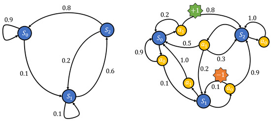
Figure 1.
Markov Process vs. Markov Decision Process.
Many planning and decision-making problems require choosing a sequence of decisions [33]. The problems that are formulated by MDPs require a known model and a fully observable environment. The MDP model consists of states, actions, rewards, transition probabilities, and discount factors. Hence, MDP is a tuple defined by:
where S is the state space, is the action space, is the transition model, is the reward model, and is the discount factor. Discount factor balances current and future rewards and smoothly reduces the impact of prompt rewards. It also enables to building of a strategy to maximize overall reward at the expense of immediate rewards. is the transition probability of getting the state by applying the action when in the state . Let denote the state, the action, and the reward at time step k. As MDP is a sequential control formulation, a trajectory can be denoted as , where the action is chosen according to a policy [34].
3.2. Multi-Agent Markov Decision Processes
Multi-agent Markov Decision Processes is an extended version of MDPs to adapt them to multi-agent problems which consist of multiple agents trying to optimize a common objective. The MMDP formulation has lots of similarities with the exception that possible decisions, namely actions, are distributed among agents in the system [35]. This formulation still requires each agent to observe the true state of the domain and coordinate on their taken actions [36]. MMDP expands the above framework to a set of n agents. An MMDP is also defined by a tuple:
where is number of agents and is a MDP with factorized action space:
where denotes the local action sets of agent and is the joint action set of the multi-agent problem [37]. Note that the size of the action space is exponential in number of agents. In many multi-agent problems, factorization of state space, transition models, and rewards of the agents are possible. By exploiting that structural property, computationally efficient algorithms can be developed [38].
State space is factorized into individual state spaces of each agent as follows:
where denotes the individual states for agent, is the state of external variable j, and is the dimension of the external states. Many real-life problems utilize this assumption, such as multi-agent traffic regulation problems, where the states of the traffic lights are associated with individual states and the position of the vehicles can be associated with external states. Transition dynamics can also be factorized as follows:
where , and , . Note that while the transition dynamics of each agent only depend on the agent’s external states, individual states, and individual actions, external transition dynamics depend on joint action space and joint space. Hence, the dynamics of the external states are not decoupled from agents, they are influenced by actions of all agents. The reward can also be decomposed as:
where each . Each local reward is individually dependent on the local states, local actions, and joint space of external states. Since MMDP is basically an MDP that has a specific structure that can be factorized, modeling multi-agent problems becomes easier. Thus, MMDP problems can be solved as an MDP. However, even factorized MMDPs have large state and action spaces that are exponential to the number of agents, those classical approaches usually do not scale well for multi-agent problems.
3.3. Reinforcement Learning
Reinforcement Learning is a class of machine learning solution methods that is highly effective with stochastic optimal control and decision-making problems which can be formulated as MDP [22]. RL problems consist of an agent that is learning the best behavior through a kind of trial–error interaction with a certain dynamic environment. It primarily focuses on how an agent should develop a policy that leads to achieve goals in a complex environment where uncertainties might exist. As RL does not always require scientists to construct a model of the problem, it allows to development of generalized algorithms that can be applied to various problems.
At each time step, the agent, being in a state, performs an action, the environment provides a reward, and the agent moves to the next state; this dataset includes state, action, and reward, and the next state is called the experience through which the agent can learn which actions lead to higher rewards [39]. A state is descriptive information of a system that covers all the information relevant to an agent’s decision-making process at a particular time. As seen in Figure 2, the dynamic environment provides a new state and a reward on each step of interaction the agent attempts with action . The overall goal of the agent is to maximize the total rewards so that the agent can optimize the policy by mapping the states to actions to perform better.
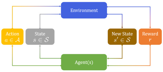
Figure 2.
Agent interacts with the environment in a reinforcement setting.
The objective of the planning problem is to find a policy by maximizing the cumulative discounted reward for a given initial state :
where is the reward at step t and is the discount factor. The value of taking an action in a state under policy, , is the expected return starting from that state, taking that action as given below:
where is the expectation operator taking over the possible next states and is the state–action value function under policy .
The Bellman equation is an optimality condition associated with DP and is widely used in RL to update the policy of an agent. The Bellman update only guarantees convergence to the optimal state–action value function if every state is visited an infinite number of times and every action is tried an infinite number of times. It can be shown that satisfies the Bellman Equation [40]:
In particular, the optimal policy is defined as:
where, for a given state, the action with the biggest value in the value function is chosen through all other action candidates. Training of RL is highly sensitive to several high-level parameters including exploration–exploitation dilemma and how the q values are stored.
3.3.1. Exploration–Exploitation Dilemma
The exploration–exploitation trade-off dilemma emerges for RL and not in other kinds of learning [22]. While the agent aims to maximize the cumulative discounted reward, it exploits its policy and it probably leads the agent to get stuck at a local optima or makes the agent never find a good policy, especially at the very beginning when the agent is uneducated. However, the exploration is to find out which actions might lead to good rewards, at the first place the agent must try actions out and run the risk of getting a penalty. The majority of practical implementations are balancing exploitation and exploration by utilizing the algorithm [41]. In this study, the algorithm has been applied with a so that the agent starts with exploration and as the learning advances it shifts to exploitation since the environment is known better.
3.3.2. Representations
The way of storing the values for state and action pairs is called representation. Representation is separated into two main groups as tabular representations and compact representations [42]. In tabular representation, each state and action pair is stored in a look-up table. This way of representation offers optimal decisions. However, due to the curse of dimensionality for large state–action spaces, this type of representation requires huge memory in practical applications [43]. This drawback pushed the researchers to move away from tabular representations to more compact representations. In compact representations, the value of each state–action pair is estimated implicitly using given features. One possibility as a compact representation is to use multilayer perceptrons such as deep neural networks to overcome the drawbacks of the curse of dimensionality to some extent.
3.4. Deep Q-Networks
Deep Q-Networks is a technique that adapts neural networks into RL to address otherwise intractable problems [44]. It is a generalizing approximation function across the state and action pairs to reduce dependency on the domain knowledge of large-scale problems with efficient use of computational resources. Recent studies on machine learning and, in particular, on deep learning have demonstrated very promising successes in solving problems with complex and high dimensional spaces [41]. DQN is capable of representing non-linear functions that RL requires to store mappings of state–action pairs to Q values. Deep neural networks are exceptionally good at coming up with good features for highly structured data. DQN could represent the Q-function with a neural network, which takes the state as input and outputs the corresponding Q-value for each action. DQN also utilizes the Experience Replay concept to successfully approximate the q values.
3.4.1. Deep Neural Networks
The Deep Neural Network is a technique inspired by how the human brain works to make it possible for machines to learn from data [45]. DNNs became more popular since they outperformed most of the current machine learning algorithms. The most significant reasons cause that neural networks can represent any smooth function at all with enough training samples [46], the back-propagation algorithm enables training the network just using simple operations over derivatives [47], and being able to get trained through GPU thus doing it outperforms CPU by far [48]. In contrast to customary neural network applications, in the reinforcement learning context, there is no readily available training set to train the algorithm. Each training label should be inferred during iterative value updates.
The network is modeled by the output function , where x is a vector of inputs and w is a vector of weights. The output function y varies with changes in the weights. Our goal is to find the weight vector that minimizes the error. The error is due to the improper values of weights resulting from a difference between the desired output and the network output for that training data pair. That pair includes an input vector x and a label vector y. Define a topology:
where m is the number of total layers and is the ith layer of the network.
3.4.2. Training with Back Propagation
Training of a network is done by following the steps given below.
- 1.
- Given a training set:where t is the total number of training pairs.
- 2.
- For each element of the training set, feed-forward the input and obtain output , then calculate the error:where d stands for dth training data and stands for number of neurons in the mth layer.
- 3.
- Then, calculate the gradient:
- 4.
- Update the weight using gradient descent:
3.4.3. Experience Replay
The fully connected network used in Deep-Q-Networks tends to forget the previous experiences as new samples are collected. As the importance of batch data processing mentioned before, the experience replay technique addresses the issue of how the elements should be selected from memory into the batch list [41]. To perform experience replay, the agent’s experiences are stored as in a memory buffer. These experience elements consist of state, action, reward, and next state. The populated memory is used to select the elements of the batch using a uniform distribution. Then, the batch list is replayed when training the network. This randomized mechanism allows the learning algorithm to be more stable by removing the correlations in the observation sequence. It also brings together a smoother convergence over the changes in the experienced data distribution.
4. Problem Description
This section introduces the definition of the delivery by multiple drone problems and investigates the details of the operation as this problem is challenging enough to demonstrate the proposed methods. The drone delivery problem has been treated as a grid-world problem. The primitive setting of the grid world problem consists of an agent, a partitioned area closed with walls, at least one reward point, and some non-compulsory blocked and penalty partitions. Our agent can move one step at a time and have five actions, including do nothing, up, down, left, and right. In order to experience uncertainty, the outcome of each action is modeled as a stochastic process [33]. As seen in Figure 3, if the agent tries to go up, it will move to the desired position with a probability of , but there is also a substantial chance it finds itself in left or right grids with a probability of . This kind of movement can be influenced by external factors, such as wind, actuator variability, and sensor precision. Therefore, the next movement can inadvertently align with the result of one of the adjacent actions (e.g., a drone moving ’left’ might drift ’up’ or ’down’ in the cell representation). This adjacency in action outcomes reflects the real-world challenges of precise control in a dynamic environment. Acknowledging these sources of uncertainty, our model aimed to capture the unpredictable dynamics, providing a simplified yet representative framework for the analysis.
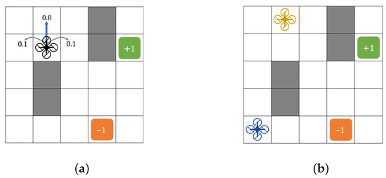
Figure 3.
Illustrative examples of primitive environments with action uncertainty utilized as a baseline in both delivery by drone simulations and evaluating hyper-parameters for the methods, i.e.,the single-agent and multi-agent grid world. (a) Single-agent grid world problem illustrating cells that can be blocked, rewarded, and penalized along with the uncertainty of the action “up”. (b) Simplified multi-agent grid world problem where agents are rewarded once agents meet the high reward cell.
If the agent bumps itself into the outer walls or blocked grids, it will stay in the same position. While reaching the goal state has a positive reward, such as , reaching the penalty states have a negative reward, such as . Since there is a small yet effective movement penalty, such as , the main object of the problem is to reach the goal state with the smallest number of steps. The row and column position of the agent represents a state for the problem. The initial state can be selected either fixed or randomly depending on the requirements of the method that will generate a solution to the planning problem.
The assumptions made during modeling the problem in this study are listed as follows:
- Any drone can travel only along the grid (not diagonally);
- Each cell in the grid is large enough to fit multiple drones, and therefore, collision is not considered;
- Take-off and landing durations are not considered;
- Only distance traveled is considered during fuel consumption, the time spent is ignored;
- Reaching out to the associated cell is sufficient for a drone to fuel up, pick up, or deliver the package;
- The agents can independently move on the grid.
4.1. Formulation
The multi-agent delivery by drone planning problem is derived from the single-agent grid world problem. The configuration is almost identical except for the number of agents and refuel stations. This planning problem is designed to evaluate the performance of algorithms that support multi-agent decision making. The main goal of such a setting is to generate such a policy that allows the agents to collaboratively seek to maximize cumulative rewards using multi-agent MDPs. Due to the multi-agent setting, each agent in fact is represented by a decision-maker agent and occupies a position in a grid. Each agent can take any of five actions to change its current position toward a goal.
In addition to primitive settings, the delivery by drone setting introduces new dimensions to the state due to the package pick-up position, delivery point, and battery consumption. Both the package and its destinations are also represented by another position in the grid. The prominent properties of the delivery by drone problems that have been considered when modeling the environment are such as refueling stations, blocked or no-fly zones, packets waiting to be picked, and the delivery point for each specific packet. In order to let the agent learn to deliver a package, a positive reward of can be provided for successfully flying to a delivery position with the packet has been picked. The notations used throughout the problem formalization section are listed in Table 1.

Table 1.
Notations used for delivery by drone problem.
4.1.1. State Space
The global state of the problem for multi-agent case , where can be decomposed as in Equation (16):
The overall state comprises individual states which are identical in terms of structure among all the agents. The state of each agent is given by several scalar variables describing the vehicle’s position, fuel state, the position of the package assigned to the vehicle, and the delivery point that the vehicle should visit with the packet. Each element in the state is given by scalar variables describing the status of vehicle and packages, where , , are the position and the fuel status of the nth vehicle, and are the position of package to be picked which is already assigned to the nth vehicle, and lastly and are the delivery points denoting the vehicle should visit just after picking up the package as listed in Table 1.
In a delivery by drone setting an agent will not be able to endlessly deliver the packages due to having limited battery capacity. With every movement of the agent the charge of the battery will decrease slightly. With the limited battery capacity, running out of power keeps the agent out of service, which results in having no more rewards. Therefore, the environment improved by placing a charging station or refueling station on the grid. Thus, the agent can fly towards the station to recharge its battery to be able to deliver more packages to have more reward. The multi-agent scenario of the delivery by drone problem has been depicted in Figure 4. The agent needs to take appropriate actions towards frequently visiting the charging stations when the battery is low even though the charging station is not on the optimal path between the agent, packet, and delivery point. If the fuel state reaches zero before visiting the refuel station, the vehicle will ignore any action and keep its last state resulting in an ineffective agent. Therefore, the fuel state at step t for the nth vehicle can be give formalized as:
where is the decrements each time an action is taken and is the max fuel state just after the initialization or refuel station is visited.
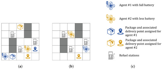
Figure 4.
Illustrative example of the delivery by drone problem. The agents, fuel stations, blocked cells, packages, and delivery points are randomly spread out to the grid at the beginning of the problem. As steps move forward, each agent makes a decision and takes an action. As a result of this, agents interact with the environment in the following ways: refuel, pick up package, deliver previously picked-up package, or cannot move anywhere due to empty fuel. (a) Randomly initialized delivery by drone problem at step with 2 sets of agents and packages, the blocked cells and fuel stations that will max out the fuel are fixed. (b) The status of the environment at step after taking optimum actions towards a collaborative goal ends up less energy left as the fuel station is not visited yet. (c) Legend for delivery by drone problem.
The packet position variables and , and delivery points and can take and , respectively, as a value unlike the other position values. It has a special meaning decoded into the state space to indicate to the algorithms that the package was picked or delivered. Both and will take when the package is picked; otherwise, both will point out the exact location of the package in the grid. Both and will take when the package is delivered; otherwise, both will point out the exact location of the delivery point for the package in the grid.
4.1.2. Action Space
The action space for nth agent depends on the status of agent’s, package’s, delivery point’s position, and fuel remaining for the vehicle. The action space for is determined as follows:
- If packet is not delivered yet, ;
- If packet is delivered and no more available, ;
- If fuel is empty, .
4.1.3. State Transition Model
The state transition model covers the qualitative description of problem dynamics given at the start of this section. It captures the probability of certain results happening after a given action thus creates uncertainty. The model given here can be partitioned into dynamics for each individual agent [49]. The dynamics for the operation of delivery by drone problem are described by the following rules:
- If the fuel is not zero, the agent moves toward the direction of action selected with a probability of by only one unit away from where it is located or moves toward the direction of one of the adjacent action indicates with a probability of .
- If the resulting action makes the agent move towards a blocked state, the agent remains in its previous state.
- If the fuel is zero, the agent remains in the same position forever with .
- If the agent reaches a position where a refueling station exists is maxed out to .
- If the agent moves to a different cell than where it is located, the fuel variable decreases by for each step.
- If the agent reaches a position where the package exists (,) = (, ), the agent will continue to transition to another cell selecting an action from in the next step and the packet states will be equal to (,) to indicate that packet is picked up.
- If the agent reaches a delivery point with a package, the agent does not transition from this state and continues to apply and both packet state and delivery point state will be set to and , respectively.
4.1.4. Reward Model
The reward model primarily promotes delivering packages. Besides that, in order to encourage picking package, achieve goals with fewer actions, and travel with fuel levels far from staying in the middle of nowhere, there are other rewards. These rewards are minor as they can cause to stuck at local maxima. Minor rewards can be achieved when fuel stations are visited and packets are picked up.
where:
- : number of packages delivered;
- : number of packages picked;
- : number of visits to the fuel station;
- : number of moves taken.
Moreover, , , , and are the relative rewards of delivering a package, picking up a package, visiting the fuel station, and penalty for taking too many actions to achieve a global goal, respectively.
5. Methodology
This section describes the methods that have been applied to the delivery by drone problem and the methods are compared in the following section. These methods are deep reinforcement learning, deep correction, and the proposed package distribution that combines the Genetic Algorithm with reinforcement learning and Curriculum Learning.
5.1. Application of Deep Reinforcement Learning
The application of Deep Reinforcement Learning (DRL) in the multi-agent delivery by drone problem is the baseline for the following enhanced methods. It is a pivotal method for enabling intelligent decision making and action selection. The network structure, as illustrated in Figure 5, serves as the foundation for this application, encompassing neural layers that facilitate the learning and representation of complex relationships within the environment.
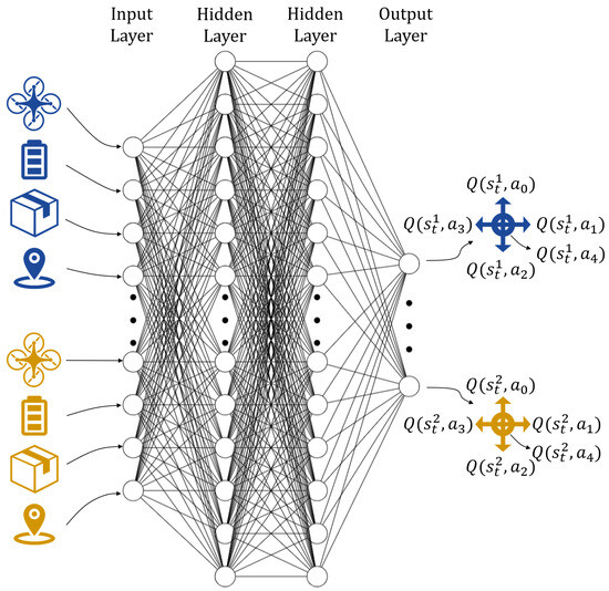
Figure 5.
An example of the network structure for multi-agent delivery drone problem with hidden layers. The input is the cascaded state vector elements including the position of the agent, remaining fuel, the position of the packet to be picked up, and the delivery point of each agent. The output is the q-value of each possible action for each agent including up, down, left, right, and do nothing.
The input to the DQN consists of a comprehensive cascaded state vector, capturing essential elements crucial for informed decision making by each agent. This state vector includes the positional information of the agent within the environment, the remaining fuel levels, the coordinates of the packet to be picked up, and the delivery destination for each agent. This holistic representation ensures that the network is equipped with a comprehensive understanding of the current environmental context and the specific tasks assigned to each agent.
The hidden layers embedded within the network structure play a vital role in capturing the intricate dependencies and patterns present in the multi-agent delivery drone problem. Through a process of supervised learning and reinforcement learning, the DQN adjusts the weights and biases of these hidden layers to approximate the optimal action–value function.
The network’s output is a set of Q-values, each corresponding to a possible action for each agent. The available actions typically encompass fundamental movements, such as up, down, left, and right, along with a ’do nothing’ option. These Q-values quantify the expected cumulative rewards associated with each possible action, providing a basis for the agent to make intelligent decisions that maximize its long-term objectives.
During the training phase, the DQN utilizes a combination of experiences from the environment and the rewards obtained through delivery by drone environment to update its parameters. The objective is to learn a collaborative policy that guides agents in selecting actions that lead to the maximization of cumulative rewards over time. The depicted network structure in Figure 5 exemplifies how Deep Q-Networks are applied to address the multi-agent delivery drone problem. By incorporating comprehensive input representations, hidden layers for learning complex relationships, and output Q-values guiding action selection, the DQN framework enables agents to navigate the environment and fulfill their delivery objectives up to a certain amount of agents within reasonable learning steps.
5.2. Prioritized Experience Replay
Prioritized Experience Replay is an extension of replay memory, which addresses which experiences should be replayed to make the most effective use of experience storage for learning [50]. Since most of the problems included in RL exhibit sparse rewards, reaching these rare rewards and making inferences about the problem requires different novel techniques. Coping with sparse rewards is one of the biggest challenges in RL [51]. One can classify the state transitions as ’surprising’ when an agent happens upon a positive reward and ’boring’ when an agent gets nothing different as the outcome of an action [52]. Therefore, some transitions have importance over the others. The learning algorithm should focus on the experiences that are more important using the prioritized experience learning to be able to learn faster.
In order to differentiate the surprising and boring transitions, PER uses the temporal difference (TD) error that simply computes the difference between target network prediction and q-network prediction to assign a priority over the received experiences [53]. A big TD error results in a higher priority:
This TD error can be transformed into a priority:
where i is the index of experience, represents the proportional priority of experience i, and is a small positive constant that prevents transitions not being revisited once their error is zero. The exponent determines how much prioritization is used, with = 0 corresponding to the uniformly selected experience as in Experience Replay. Then the priority can be translated to a probability, so one can simply sample it from the replay memory using its probability distribution. An experience i has the following probability of being picked from the replay memory:
When a problem requires large datasets and memory buffers, searching from memory for the element that has the highest priority can be intractable in practice with usual data structures. The sum-tree is a commonly used data structure for PER and it offers the search to be completed at complexity. In sum-tree, the value of a parent node is the sum of its children. Only leaf nodes store the transition priorities and the internal nodes store the sums of their own child. To sample a minibatch of size k, the range is divided into k ranges [50]. Then, a value is uniformly sampled from each range.
5.3. Utility Decomposition with Deep Correction Learning
In the past, decomposition methods were suggested as a way to estimate solutions for complex decision-making problems that occur sequentially [54]. In situations where an agent interacts with multiple entities, a technique called utility decomposition can be utilized. This approach considers each entity separately, calculating their individual utility functions. These individual functions are then combined in real time to solve the overall problem while sacrificing optimality. Deep-neural-network-based correction methods are then applied to learn correction terms to improve the performance [55].
5.3.1. Utility Decomposition
Utility decomposition consists of the process of breaking down the complex formulation of a problem into simple decision-making tasks. Each subtask is then solved separately in isolation. As solving the global problem suffers from the curse of dimensionality, solving each isolated subtask requires exceptionally less computation power [55]. At the end of the process each solution is combined through an approximate function f, also named the utility fusion function, such as:
where is the optimal value function of the global problem and n denotes the subtask id. According to [55], for the independent agents two approximation functions, max-sum and max-min, can be utilized to combine the subtask solutions:
This approach equally weighs the Q-Values of each agent. Instead, another strategy is to consider taking the minimum as follows:
In this study, the first approach is focused on the sake of simplicity and evaluated the performance of the decomposition method with respect to regular deep q-networks.
5.3.2. Deep Correction
This technique makes use of the decomposed utility functions to guide the RL agent toward an ideal policy while using less training data [55]. The architecture of the deep correction method is depicted in Figure 6. The method is inspired by the multi-fidelity optimization [56]. The composed model is evaluated as and the model that takes into account the deep correction network is considered as a part of , as given in Equation (26). The deep correction network is the additive part that is nothing but another DQN.

Figure 6.
Architecture of decomposed deep correction network. The global state is decomposed into substates that represent each agent, and the substates are fed into pre-trained single-agent networks. In order to approximate the global Q-function, the output of the utility fusion is combined with the output of the deep correction network.
The global functıon can be given as the sum of low fidelity model and the correction term as follows:
The cost function that needs to be optimized with respect to will be:
where can defined as the updated value as:
The gradient of the cost function can be derived with respect to the network parameters of the correction network:
Substituting Equation (28) into gradient will give:
Substituting Equation (26) makes the gradient as given below:
As does not change with , the resulting gradient function will become:
The gradient descent update rule will optimize parameter as given below:
Therefore, taking the gradients with respect to trainable parameters, the update rule becomes as following:
5.4. Curriculum Learning
Curriculum learning is a technique in RL that involves gradually increasing the difficulty of the tasks or environments faced by an RL agent as it learns and improves. By starting with simpler tasks and gradually moving on to more complex ones, the agent can learn more effectively and generalize faster. The gradual increase in difficulty allows the agent to build up its skills and knowledge gradually, rather than being overwhelmed by trying to learn too much at once. When the given task is complex due to opponents, suboptimal representations or sparse reward settings learning can be remarkably slow [57]. It also allows the agent to focus on specific aspects of the task at a time, which can help prevent overfitting and ensure that the agent generalizes well to new situations. It would be beneficial to have the learning process focus on examples that are more valuable and neither too challenging nor too simple [58]. Therefore, this technique helps an RL agent to learn and adapt to new environments and tasks, and can be particularly useful in scenarios where the agent needs to operate in complex or dynamic environments [59]. In the end, all the knowledge is transferred to the learning task that is targeted at learning the main problem.
Agents in standard reinforcement learning start to learn the environment through random policies to find a policy that is close to the optimal policy for a given task. In the curriculum learning setting, instead of directly learning a difficult task, the agent is exposed to simplified versions of the main problem [60]. In the context of a planning problem, Curriculum Learning could involve starting with a simple environment where the agent has to navigate simple, straightforward routes and deliver packages to fixed locations. As the agent learns to perform this task well, the environment could be made more complex, for example by introducing obstacles or dynamic elements such as moving vehicles.
For the delivery by drone problem, there are several levels that can be exploited for Curriculum Learning. These levels can be as given below:
- Navigating around the map: Initially, the agent learns to navigate the spatial layout efficiently, mastering the basics of pathfinding and map traversal.
- Picking up the packet and providing delivery: The curriculum then advances to include the intricate tasks of package pickup and delivery. This step builds on the navigation skills acquired in the previous level, introducing additional complexity.
- Consuming fuel or energy during the operation: The final level involves incorporating the consideration of fuel or energy consumption, further augmenting the challenge. This aspect becomes critical in addressing real-world constraints and optimizing the drone’s operational efficiency.
5.5. Package Distribution with Genetic Algorithms
Genetic Algorithms are a type of optimization algorithm inspired by natural evolution and can be used to solve a wide range of decision-making problems, including those in the field of reinforcement learning [61]. GAs are used to find approximate solutions to complex problems that are difficult or impossible to solve using traditional methods. GAs start with a population of potential policies (i.e., sets of rules or decision-making criteria) for the decision maker to follow. It would then evaluate the performance of each policy by simulating the actions in the environment and measuring the rewards they receive through fitness functions. The GA would then use this information to determine which policies are the most successful and select those for reproduction and further optimization. Over time, the GA would iteratively improve the policies through a process of selection, crossover (i.e., combining elements of successful policies to create new ones), and mutation (i.e., making small random changes to the policies to introduce new ideas and avoid getting stuck in local optima). The ultimate goal would be to find a policy that allows the agents to maximize their rewards and achieve their global objectives as efficiently as possible. Using a GA in this way can be particularly useful in situations where the decision-making policies for the agents are complex and there are many possible actions they can take, as it allows the algorithm to explore and optimize a large search space in an efficient and effective manner.
In the context of the delivery by drone problem, the GA could be used to optimize the decision-making policies of multiple drones operating in the same environment. This could involve using the GA to search for the best possible actions for each drone to take at each time step, based on the current state of the environment and the rewards being received by the drones. In case the number of packets and drones is limited to a few numbers, the calculation of permutation that is required to assign each packet to a drone is tractable. On the other hand, if the number of agents increases the number of fitness values that need to be calculated increases exponentially as well. For instance, the number of fitness values that need to be calculated is if the number of agents is 10 for each single simulation of packet assignment. In this case, an efficient packet distribution becomes intractable if all fitness values are considered. Therefore, the packet distribution has been optimized with GA as given in Figure 7. As Genetic Algorithms provide optimization over large space states, they simulate the process of natural selection to find high-quality solutions for optimization and search problems.

Figure 7.
Genetic-algorithm-aided packet distribution framework combined with pre-trained deep reinforcement learning agents. The input of the framework is the cascaded states of each agent, which includes packets and delivery points randomly assigned to agents. GA permutes the package delivery tasks between agents and seeks the optimal permutation through a loop that includes selection, crossover, and mutation. The resulting permutation gets converted into a cascaded state again with each packet delivery task optimally assigned to each agent. Finally, the agents carry out their delivery task independently towards a global reward.
In order to resolve the packet distribution with a Genetic Algorithm for a high number of agents, key components of the algorithm, including genome, chromosome, and population, should be represented by the problem [62]. For our packet delivery problem, a chromosome is mapped into nth permutation of the vector, which reflects which drone will carry which packet. In this case, a genome becomes just a number that reflects the id of the packet and the population becomes a set of random chromosomes with a predefined length which is 20 for this problem. The very first input and the optimal output of the Genetic Algorithm can be expressed as given below:
There are other operators of Genetic Algorithms, such as Fitness, Selection, Crossover, and Mutation, that need to be represented as well. For the fitness operator, the cumulative reward of the simulation has been utilized. The selection operator is the one that aims to find two parents that will generate offspring chromosomes through the crossover. Parents have been found by ordering the population by their fitness values. As this packet distribution problem is represented by permutation, conventional crossover operators lead to inadmissible solutions. Therefore, Order One Crossover has been utilized to keep the properties of permutation valid. In order to avoid premature convergence, Single Swap Mutation has been applied.
Each simulation starts with a certain amount of agents and packages. Since the packets and agents are distributed randomly, the performance of the overall simulation will likely be poor due to various factors such as the distance to the agent and refueling stations. Before starting the simulation with randomly assigned drone pairs, a package distribution algorithm runs. It basically permutes the candidates of the package, agent pairs, and then calculates the fitness value for each pair. The state and fitness values are placed into a dictionary. At the end of visiting each state, the state with highest fitness value within the dictionary is returned.
5.6. Execution
The execution of the proposed system’s workflow can be described with distinct phases. This segmentation clarifies the overall operational framework and highlights the efficiency embedded in each stage. The process is divided into three main phases: the Initial Training Phase, the Packet Distribution Phase, and the Execution of Delivery Tasks Phase. While the Initial Training Phase involves a one-off, more time-consuming computational process, the subsequent phases are optimized for speed and efficiency, ensuring real-time responsiveness in the dynamic environment of drone delivery. Each phase contributes to the system, balancing the upfront computational investment with real-time operational capabilities.
- Initial Training Phase: The model incorporates DQN, PER, and Curriculum Learning, which require a significant amount of computational time for the initial training. However, this is a one-time process, taking substantial amount of hours to complete for the map that incorporates no-fly zones and refuel stations. Once the training is finalized, the model does not need to be retrained unless there is a substantial change in the operational environment.
- Packet Distribution: After the initial training, the model employs a Genetic Algorithm for packet distribution among agents. This step is computationally efficient and takes seconds to minutes to complete depending on the setting. It is designed to quickly adapt to the dynamic requirements of real-time delivery tasks.
- Execution of Delivery Tasks: Each drone independently executes its delivery tasks based on the pre-trained model called the inference model. This inference phase is extremely fast, occurring in milliseconds. Hence, once the delivery tasks are assigned, agents can promptly carry out their operations, ensuring the real-time responsiveness of the system.
By separating the computationally intensive training phase from the real-time operational phase and employing efficient algorithms for packet distribution, the proposed solution maintains real-time efficiency in defining and executing routes. This architecture ensures that while the very initial setup for the environment requires time, the actual operational phase aligns with the real-time constraints of delivery by drone systems.
6. Simulation Results
In this section, results of the simulations conducted to evaluate the performance of various methods in addressing the delivery by drone problem are presented. The methods considered are DQN, prioritized experienced replay, decomposition with correction, and GA-aided packet distribution methods. To provide a comprehensive analysis, the results are presented in order of increasing complexity, offering insights into the efficacy of each method under varying conditions.
6.1. Grid World Rendezvous Problem
The DQN algorithm is validated on a multi-agent setup on 5 × 5 grid world where agents are expected to meet at rendezvous point to reach a global goal with different neural network parameters under uncertainty. The two DQN’s with different hidden layers have successfully learned how to act on the environment. When compared with the tabular representation, which is optimal but not tractable for bigger environments with more interactions between high number of agents, the first DQN had parameters and the next had parameters of the tabular representation to be able to capture the learning task. The weights, biases, and neurons in the layers are the major factors that identify the number of parameters needed to be trained. Figure 8 shows that the DQN with fewer parameters can also learn the task but converges with an acceptable delay.
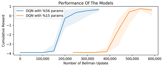
Figure 8.
Multi-agent simulation with two different deep q networks compared against each other with different numbers of neurons configured relative to tabular approach.
The hyper-parameters, such as batch size, replay buffer size, hidden layers, and epochs, play a crucial role in the training process [41]. Table 2 lists the parameters that are utilized within a grid search to find optimal values along with the Mean Squared Error (MSE). The MSE is a measure of the quality of convergence to 1 and lower MSE indicates that the learning performance with given hyper-parameters is better. Figure 9 shows multi-agent simulation results in a 5 × 5 rendezvous environment. The visualization presents a comparison of the convergence rates of 36 different learning algorithms through their mean squared error (MSE) values, using a logarithmic scale for enhanced clarity to focus better on lower values. This scale allows us to identify differences among the lower values, which are critical for evaluating model performance. The Model #2 with the lowest MSE, highlighted in red, clearly stands out as the best performer among the group, indicating the most accurate predictions. The logarithmic scale emphasizes the substantial variance in performance across models, with some models having significantly higher errors, depicted through the use of exponential y-ticks to accommodate the wide range of MSE values. The 5 × 5 environment has been utilized as a benchmark environment to validate the implementation of various components of DQN, as the larger settings are computationally expensive to run in gridsearch for multiple agents. Upon demonstrating the implementation works as expected, the abovementioned components are challenged with the 10 × 10 setting with the same hyper-parameters captured in a 5 × 5 environment, such as batch size, replay buffer, and epocs. The hidden layers have been increased to improve the learning capacity of the model.
Table 2.
Hyper-parameters sought in a grid search in a 5 × 5 rendezvous setting to have insight into the sensitivity of the parameters. The parameter set that made the learning converged fastest is indicated with *.
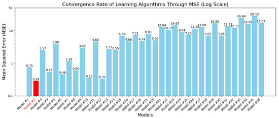
Figure 9.
Grid search results to find the best hyper-parameters of DQN with experience replay in 5 × 5 Rendezvous setting with two agents. The hyper-parameters of Model #2 performed best against MSE.
Figure 10 shows a comparison of different experience replay settings for the same multi-agent grid world problem with DQN. As the value goes from 0 to 1 as given in Equation (22), the prioritization becomes more effective than the uniform selection of experiences. Prioritized Experience Replay demonstrates that it is highly efficient for learning tasks to converge to an optimum state faster. Figure 10 shows that PER converges dramatically faster than the Uniform Experience Replay.
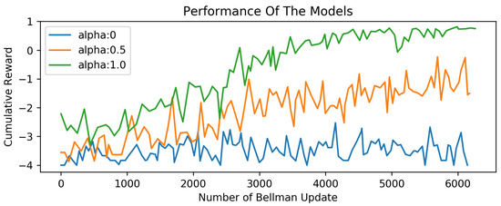
Figure 10.
Simulations results with different alpha parameters of prioritized experience replay: as alpha goes to 1, the prioritized experience replay becomes more effective than the traditional experience replay.
In order to evaluate the performance of the DQN and deep correction method with PER in a multi-agent setting, the delivery by drone problem formalized in previous sections has been utilized as a more complex task. The performance of the method has been delivered through the evolution of the policy during training. The evolution can be easily followed by a graph that shows the cumulative reward with respect to the number of Bellman updates. Several types of environments have been experimented with to find the capabilities and limits of each method in terms of scalability against number of agents. The major parameters taken into account during the simulations are the size of the grid and the number of agents.
6.2. Delivery by Drone Problem
To run the deep correction network, a single agent policy should be generated through DQN, as given in Figure 11 for the grid with size of 5 × 5. The single agent with DQN can successfully reach a good policy at a reasonable Bellman Updates for delivery by drone problem. The deep correction network has been enabled for the multi-agent settings and other agents have been invited into the game. As can be seen in Figure 11, the method performed well and maintained good learning stability at acceptable Bellman updates. Hereby, it is also demonstrated that learning a successful policy in the multi-agent setting with the corrective factor can be done with far fewer training samples. Otherwise, traditional methods such as DQN could take several orders of Bellman updates to reach the same performance since it directly learns the value function of the full-scale problem at once, as can be seen from the bad performance of DQN even with PER in Figure 12b (red) for the three-agent case.
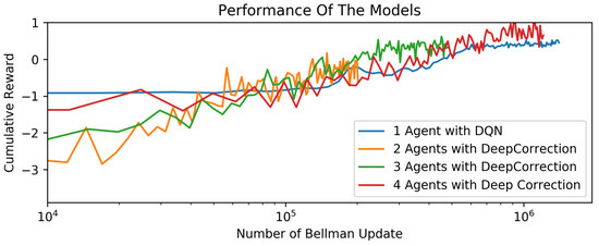
Figure 11.
Learning performances of delivery drone in 5 × 5 environment for one agent ( states), two agents ( states), three agents ( states), and four agents ( states).
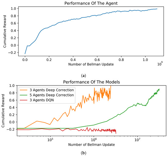
Figure 12.
Learning performances of delivery by drone in a 10 × 10 environment. (a) Single agent with DQN. One agent ( states) with DQN with PER converges to a good reward but took a substantial amount of time. (b) Deep Correction vs. DQN for multiple agents. Three agents ( states) and five agents ( states) with the Deep Correction method along with three agents with the DQN method and PER. The deep correction method outperforms the DQN method for the three-agent case and converges a high cumulative reward for five agents as well.
The same problem with higher state and action space could also utilize the deep correction method. The environment of delivery by drone in 10 × 10 grid with a single agent already has around states. The multi-agent version of the delivery by drone problem exponentially grows in state space, which is intractable with traditional reinforcement learning techniques. For example, while the delivery by drone problem with two agents has states, the same environment with five agents will have states. Figure 12a shows the learning performance of a single agent delivery by drone problem in a 10 × 10 grid. The DQN algorithm required 1.2 × 10⁹ Bellman updates to converge.
Figure 12b (orange) shows the multi-agent simulation with deep correction enabled for three agents. In the three-agent cases, the learning process has been completed with less than 2 × 10⁶ Bellman updates given the single agent learning has already been completed. The capacity issue observed in the environment with 10 × 10 size. As can be seen in Figure 12b (green), the learning process performed poorly for five agents in a 10 × 10 environment.
Figure 12b (green) shows the good learning performance of five agents. The learning capacity has been improved by increasing the hidden neurons from 64 × 256 × 64 to 256 × 1024 × 2048. For the five-agent case, where the size of the state space is around , the learning progress has been completed around 3.5 × 10⁷ Bellman updates. It can be seen that the utilization of the deep correction method, ultimately increased the learning performance. Its impact on the performance can be understood better when compared to the number of Bellman updates required to complete single-agent systems and multi-agent systems, although the state and action space increases exponentially.
Figure 13 shows the learning performance of Curriculum Learning and the traditional DQN. While Model#1 (blue line) depicts the performance of Curriculum Learning, Model#2 (orange line) demonstrates the performance of the agent trained by DQN. Each notch in the curriculum case shows the switches between the levels mentioned above. It can be seen that the Curriculum Learning performs better than the other. It reaches the levels that the naive DQN will reach sooner after seeing many more experiences.
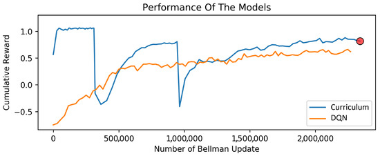
Figure 13.
Curriculum learning performance for the delivery by drone problem (the pointer shows the snapshot model that is used in Figure 18).
Figure 14 shows the performance of the package distribution algorithm given at Section 5.5 along with the initial state without any modification and randomly distributing the packages. It can be clearly seen that distributing packages through calculating the fitness value of each agent and packet pair outperforms all other combinations. The (blue) data that show packet-as-given is the default permutation mapping that maps the first agent to the first packet task and so on, which is not different from randomly assigning each packet to agents.
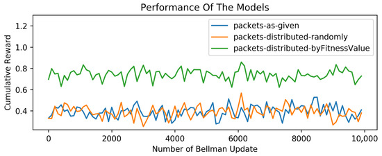
Figure 14.
The performance of the package distribution enabled setting versus the standard initialization for three agents.
Figure 15 depicts the comparison of packet distribution setting and standard initialization for two and four agents. It can be seen from the simulation results that the fitness-based packet distribution with Genetic Algorithm converges faster than the standard initialization for both two- and four-agent settings.

Figure 15.
Comparison of two- and four-agent settings with packet distribution and standard initialization.
Figure 16 shows the performance of the 10 agents trained by DQN with curriculum, PER, and packets distributed by Genetic Algorithm. Applying the Genetic Algorithm to 10 agents showed practical improvements of around , which was not possible with previous methods investigated in this study for 10 agents.
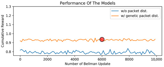
Figure 16.
Performance of Genetic Algorithm within packet delivery with 10 agents (the pointer shows the snapshot model that is used in Figure 18).
Figure 17 illustrates the computational time analysis of various multi-agent approaches investigated for a 10 × 10 drone delivery environment. The convergence times varied on a computing environment with Intel i7 CPU and Geforce GTX 1080 GPU. (Both components were acquired through project funding, as detailed in the appendix. Intel Corporation, headquartered in Santa Clara, CA, USA, manufactures the CPU, and the GPU is produced by Nvidia Corporation, also based in Santa Clara, CA, USA.) Figure 17a illustrates the convergence time in hours for various configurations of agents using DQN and Deep Correction. It highlights the scalability and efficiency challenges when increasing the number of agents, with a clear 24-h time limit, under which certain complex configurations failed to converge. The single-agent DQN model with curriculum enhancement presented a baseline for the computational time needed and other algorithms. The training of DQN configuration with the three-agent setup immediately failed to converge within the 24-h threshold. Although the configurations of three agents and five agents with the Deep Correction approach demonstrated promising convergence times, the 10-agent setting could not provide a solution within the time limit.

Figure 17.
Convergence time and packet distribution completion time analysis for multi-agent approaches investigated in a 10 × 10 delivery by drone environment underscores the trade-offs between agent count and algorithmic sophistication. (a) Computational time spent during training of each algorithm in hours, the base model reused in Deep Correction and GA showed with an asterisk. (b) Completion of packet distribution showed in minutes, inference for decision making took only milliseconds.
Figure 17b shows the completion time of GA for packet distribution and inference time spent for decision making for 10-agent settings. Multi-agent configurations with Packet Distribution through GA demonstrated balanced performance, indicating an efficient synergy between agent count and algorithmic complexity. The GA utilizes the underlying curriculum-based single-agent model and completes the packet distribution task in a reasonable time amount of minutes for a 10 × 10 environment. On the other hand, the inference element in the figure demonstrates that agents can leverage the pre-trained model for swift decision making, with inference times in milliseconds even for a complex 10-agent system. This underscores the practical applicability and real-time responsiveness of our model, making it highly suitable for dynamic and time-sensitive drone delivery operations in urban environments. This pattern underlines the critical balance between the number of agents and the chosen algorithm, illuminating the complexities in scaling multi-agent systems for drone delivery tasks.
The simulation environment for the multi-agent delivery by drone problem is visualized in Figure 18, with detailed snapshots captured at , , and . Within the confines of a 10 × 10 grid, 10 agents collaboratively navigate, picking up packets, making deliveries, and consider fuel consumption. The simulation incorporates advanced techniques, including DQN with prioritized experience replay, Curriculum Learning, and a Genetic Algorithm for efficient packet distribution. Notably, the decision-making model developed through Curriculum Learning, illustrated in Figure 13, plays a crucial role in guiding the agents. Additionally, the Genetic Algorithm ensures optimal packet distribution, as demonstrated in Figure 16. The snapshots at and showcase the synchronized efforts of the multi-agent decision maker, effectively advancing towards the global goal of delivering every package with efficiency.
However, upon closer inspection of the agents’ trajectories, it becomes apparent that certain agents, specifically those highlighted in red, magenta, green, and blue, deviate from the optimal path due to inherent action uncertainties. Notably, despite all agents successfully picking up packets, challenges arise as a consequence of unoptimized and randomly distributed fuel stations. This results in some agents, initially equipped with a fuel capacity of 10, failing to reach their delivery destinations due to premature fuel depletion.
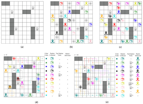
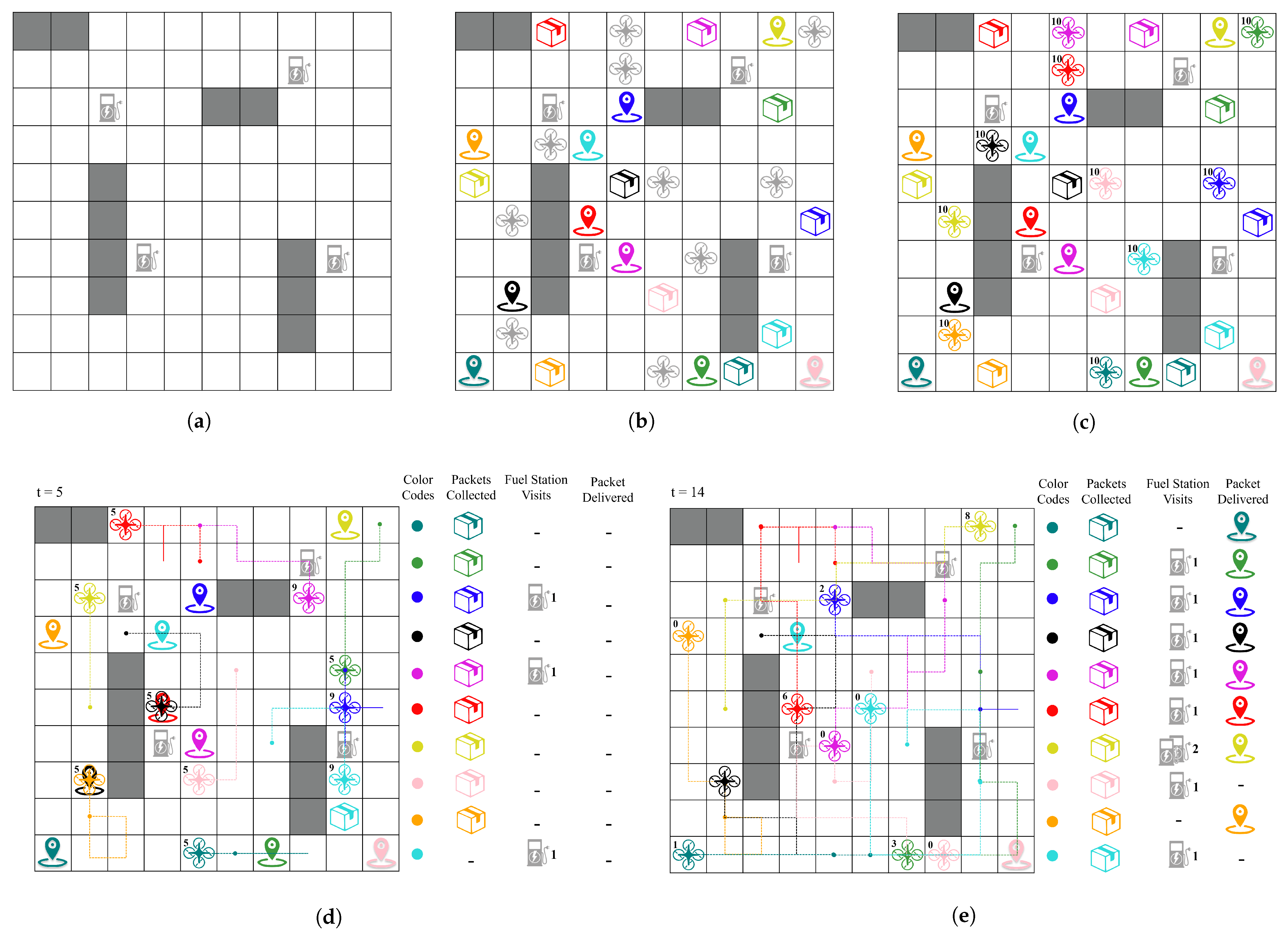
Figure 18.
Detailed visualization of the simulation environment and the snapshots at , , and . The delivery problem is simulated within a multi-agent setting of 10 agents working towards picking the packets and making the delivery to the target cells with fuel consumption considered within the 10 × 10 grid. The deep correction with prioritized experience replay, Curriculum Learning, and Genetic Algorithm for packet distribution are enabled. The agents are getting the benefit of the decision maker developed upon Curriculum Learning as frozen in Figure 13. The Genetic Algorithm handles the packet distribution efficiently as given in Figure 16. As can be seen in the snapshots of and , the multi-agent decision maker performing towards the global goal of getting every package delivered efficiently. (a) 10 × 10 grid template that agents are trained on with fixed fuel stations and blocked positions. (b) Ten randomly spawned packets, delivery points, and drones, agents are not assigned to a delivery task yet. (c) Agents are assigned to a delivery task by Genetic Algorithm at with 10 unit of initial fuel. (d) Snapshot of the environment upon collaborative actions taken by each individual agent at , where nine packets have been collected (where only the agent with cyan color is very close to capturing the packet, as it had to go around the blocked cells), none of the packets have been delivered yet, and 3 agents (blue, magenta, and cyan) visited fuel stations already and filled their fuel to the maximum unit of 10 at the time of visit. (e) Snapshot of the environment at , where all 10 packets have been captured, 8 agents successfully delivered the package and completed their task, 7 agents visited fuel stations one time, and only the yellow agent visited two fuel stations, and one agent with cyan color and one agent with pink color ran out of fuel before reaching the delivery point.
7. Conclusions and Future Work
In this paper, the challenges of multi-agent planning problems have been investigated in terms of domain knowledge, uncertainty, and scalability and a decision-making framework for autonomous packet delivery by drone has been presented. In order to mitigate the effects of the mentioned challenges, several methods including DQN, state decomposition, deep correction, Curriculum Learning, prioritized experience replay, and Genetic Algorithm have been explored and simulation results have been depicted. Each component mentioned resulted in better performance and contributed to the success rate of the learning agent and achieving a global task collaboratively. The research undertaken on the 10 × 10 grid for drone delivery has demonstrated promising potential for scalability and adaptability to various urban environments. This structured approach, investigated within the confines of a manageable yet comprehensive grid size, paves the way for its application on a broader scale. It is envisioned that this model can be conceptually placed onto diverse urban landscapes, effectively mirroring the logistics and spatial dynamics of cities in a practical manner.
While the naive DQN method cannot reach a solution even for three agents in a 10 × 10 delivery by drone setting within a reasonable amount of steps, the deep correction method successfully converged after Bellman updates. Moreover, utilizing the deep correction method increased the learning capacity to five agents and converged around Bellman update. However, the deep correction method cannot converge within the 10 agents setting in a tractable manner. Utilizing a robust computing setup, it reveals that while single-agent models establish a foundational computational benchmark, increasing agent count introduces complexity, as evidenced by the immediate convergence challenges in a three-agent DQN setup. While three- and five-agent configurations using Deep Correction show promise, the 10-agent model exceeds the 24-h convergence threshold, underlining the critical balance between agent quantity and computational feasibility.
The delivery by drone simulation results in complex settings, such as no-fly-zones, limited fuel, and the pick-and-place scenario, which showed that the proposed method with packet distribution through the GA can effectively reduce the problem to resolve the task for 10 agents in min. The reduced problem was then executed by DQN inference models aided with Curriculum Learning and PER in milliseconds. The two-folded proposed method learned the dynamics of the delivery problem without any need for domain knowledge input in an uncertain environment where actions can be altered by the environment. It is also shown through the snapshots taken in various time steps during execution that with the help of the packet distribution component realized by the Genetic Algorithm, the proposed base DQN model with Curriculum Learning and PER framework could scale to 10 agents, which was impossible with the other explored solutions within an acceptable time frame and computing resources. The proposed approach demonstrated substantial progress in multi-agent delivery by drone systems, yet our solution has limitations, particularly when it comes to addressing more complex constraints, such as extreme environmental conditions on drone reliability, dynamic packet distribution, and obstacle and collision avoidance. The framework’s robustness against certain uncertainties falls short in scenarios involving mechanical failures or operational disruptions. Moreover, the need for incorporating maintenance and repair logistics for drones, alongside investigating more intricate operational challenges, underscores the importance of further research. These areas of focus are vital for advancing drone delivery technologies to handle the complexities of real-world applications, thereby improving their scalability, efficiency, and reliability in urban environments.
The paper presents a nuanced exploration of multi-agent drone delivery systems, analyzing algorithms such as DQN, Deep Correction, and GA. It highlights the differences in learning performance, noting the advantages of Curriculum Learning and PER over traditional DQN. The computational time analysis underlines the limitations of current approaches and the necessity of efficient algorithms for real-time decision making, crucial for practical urban delivery scenarios. The analysis of a 10 × 10 grid which can be stretched as required, considering the capabilities of commercial drones and infrastructure such as charging stations, mirrors the logistical realities of metropolitan areas, showcasing the model’s scalability and practical applicability in urban contexts. This work explored a specific subset of the possible multi-agent applications, and the proposed decision-making framework offers promising directions for more complex settings. The complexities introduced by uncertainties in actions and fuel distribution underscore the significance of fuel-focused strategies and optimization algorithms in addressing real-world challenges within the multi-agent delivery by drone problem. The future work includes applying our methodology to a problem where continuous state and action spaces exist, refueling, and no-fly zones can be dynamic and agents collaboratively exchange some amount of fuel during the operation.
Supplementary Materials
The code used for analysis is provided in a repository at doi: https://doi.org/10.6084/m9.figshare.25114223.
Author Contributions
Conceptualization, writing—original draft, F.A.T.; supervision, N.K.U. All authors have read and agreed to the published version of the manuscript.
Funding
This research was funded by ‘Bilimsel Araştırma Projeleri Birimi, İstanbul Teknik Üniversitesi’, with grant number MDK-2018-41070.
Informed Consent Statement
Not applicable.
Data Availability Statement
Data are contained within the article and Supplementary Materials.
Conflicts of Interest
The funders had no role in the design of the study; in the collection, analyses, or interpretation of data; in the writing of the manuscript; or in the decision to publish the results.
Abbreviations
The following abbreviations are used in this manuscript:
| UAV | Unmanned Aerial Vehicle |
| MPC | Model-Based Predictive Control |
| DP | Dynamic Programming |
| MDP | Markov Decision Processes |
| MMDP | Multi-Agent Markov Decision Processes |
| RL | Reinforcement Learning |
| DRL | Deep Reinforcement Learning |
| DQN | Deep Q-Network |
| DNN | Deep Neural Networks |
| PER | Prioritized Experience Replay |
| GA | Genetic Algorithm |
| MSE | Mean Squared Error |
References
- Jonas, A.; Shanker, R.; Liwag, K.; Sharpe, M.; Kovanis, B. eVTOL/Urban Air Mobility TAM Update: A Slow Take-Off, However, Sky’s the Limit. 2021. Available online: https://advisor.morganstanley.com/the-busot-group/documents/field/b/bu/busot-group/Electric%20Vehicles.pdf (accessed on 22 November 2023).
- Buşoniu, L.; Babuška, R.; De Schutter, B. Multi-agent Reinforcement Learning: An Overview. In Innovations in Multi-Agent Systems and Applications-1; Srinivasan, D., Jain, L.C., Eds.; Springer: Berlin/Heidelberg, Germany, 2010; pp. 183–221. [Google Scholar] [CrossRef]
- Hessel, M.; Modayil, J.; van Hasselt, H.; Schaul, T.; Ostrovski, G.; Dabney, W.; Horgan, D.; Piot, B.; Azar, M.; Silver, D. Rainbow: Combining Improvements in Deep Reinforcement Learning. arXiv 2017, arXiv:1710.02298. [Google Scholar] [CrossRef]
- Mnih, V.; Kavukcuoglu, K.; Silver, D.; Graves, A.; Antonoglou, I.; Wierstra, D.; Riedmiller, M. Playing Atari with Deep Reinforcement Learning. arXiv 2013, arXiv:1312.5602. [Google Scholar] [CrossRef]
- Zhang, K.; Yang, Z.; Başar, T. Multi-Agent Reinforcement Learning: A Selective Overview of Theories and Algorithms. arXiv 2019, arXiv:1911.10635. [Google Scholar] [CrossRef]
- Zhu, P.; Dai, W.; Yao, W.; Ma, J.; Zeng, Z.; Lu, H. Multi-Robot Flocking Control Based on Deep Reinforcement Learning. IEEE Access 2020, 8, 150397–150406. [Google Scholar] [CrossRef]
- Tang, J.; Song, J.; Ou, J.; Luo, J.; Zhang, X.; Wong, K.K. Minimum Throughput Maximization for Multi-UAV Enabled WPCN: A Deep Reinforcement Learning Method. IEEE Access 2020, 8, 9124–9132. [Google Scholar] [CrossRef]
- Pan, Y.; Jiang, H.; Yang, H.; Zhang, J. A Novel Method for Improving the Training Efficiency of Deep Multi-Agent Reinforcement Learning. IEEE Access 2019, 7, 137992–137999. [Google Scholar] [CrossRef]
- FlyCart 30. 2024. Available online: https://www.dji.com/global/flycart-30 (accessed on 28 January 2024).
- Urbina-Brito, N.; Guerrero-Sánchez, M.E.; Valencia-Palomo, G.; Hernández-González, O.; López-Estrada, F.R.; Hoyo-Montaño, J.A. A predictive control strategy for aerial payload transportation with an unmanned aerial vehicle. Mathematics 2021, 9, 1822. [Google Scholar] [CrossRef]
- Hernández-González, O.; Targui, B.; Valencia-Palomo, G.; Guerrero-Sánchez, M. Robust cascade observer for a disturbance unmanned aerial vehicle carrying a load under multiple time-varying delays and uncertainties. Int. J. Syst. Sci. 2024, 1–17. [Google Scholar] [CrossRef]
- Clement, B. Multi-Agent Planning; Artificial Intelligence Group, Jet Propulsion Laboratory: Pasadena, CA, USA, 2004. [Google Scholar]
- Stone, P.; Veloso, M. Multiagent Systems: A Survey from a Machine Learning Perspective. Auton. Robot. 2000, 8, 345–383. [Google Scholar] [CrossRef]
- Tomlin, C.; Pappas, G.J.; Sastry, S. Conflict resolution for air traffic management: A study in multiagent hybrid systems. IEEE Trans. Autom. Control 1998, 43, 509–521. [Google Scholar] [CrossRef]
- Swaminathan, J.M.; Smith, S.F.; Sadeh, N.M. Modeling supply chain dynamics: A multiagent approach. Decis. Sci. 1998, 29, 607–632. [Google Scholar] [CrossRef]
- Glavic, M. Agents and Multi-Agent Systems: A Short Introduction for Power Engineers; Technical Report; Electrical Engineering and Computer Science Department, University of Liege: Liege, Belgium, 2006. [Google Scholar]
- MacKenzie, D.C.; Arkin, R.C.; Cameron, J.M. Multiagent mission specification and execution. Auton. Robot. 1997, 4, 29–52. [Google Scholar] [CrossRef]
- Crammer, K.; Kearns, M.; Wortman, J. Learning from multiple sources. J. Mach. Learn. Res. 2008, 9, 1757–1774. [Google Scholar]
- Chevaleyre, Y.; Dunne, P.; Endriss, U.; Lang, J.; LemaÃŽtre, M.; Padget, J.; Phelps, S.; Rodrigues-Aguilar, J.; Sousa, P. Issues in Multiagent Resource Allocation. 2005. Informatica 2005, 30, 3–31. [Google Scholar]
- Boyan, J.A.; Littman, M.L. Packet routing in dynamically changing networks: A reinforcement learning approach. In Proceedings of the 6th International Conference on Neural Information Processing Systems, Denver, CO, USA, 29 November–2 December 1993; pp. 671–678. [Google Scholar]
- Thrun, S.; Burgard, W.; Fox, D. Probabilistic Robotics; Massachusetts Institute of Technology: Cambridge, MA, USA, 2005. [Google Scholar]
- Sutton, R.S.; Barto, A.G. Reinforcement Learning: An Introduction; MIT Press: Cambridge, MA, USA, 2018. [Google Scholar]
- Tampuu, A.; Matiisen, T.; Kodelja, D.; Kuzovkin, I.; Korjus, K.; Aru, J.; Aru, J.; Vicente, R. Multiagent Cooperation and Competition with Deep Reinforcement Learning. arXiv 2015, arXiv:1511.08779. [Google Scholar] [CrossRef] [PubMed]
- Busoniu, L.; Babuska, R.; De Schutter, B. A comprehensive survey of multiagent reinforcement learning. IEEE Trans. Syst. Man Cybern. Part C Appl. Rev. 2008, 38, 156. [Google Scholar] [CrossRef]
- Zhan, G.; Zhang, X.; Li, Z.; Xu, L.; Zhou, D.; Yang, Z. Multiple-uav reinforcement learning algorithm based on improved ppo in ray framework. Drones 2022, 6, 166. [Google Scholar] [CrossRef]
- Yin, Y.; Guo, Y.; Su, Q.; Wang, Z. Task Allocation of Multiple Unmanned Aerial Vehicles Based on Deep Transfer Reinforcement Learning. Drones 2022, 6, 215. [Google Scholar] [CrossRef]
- Ding, C.; Zheng, Z. A Reinforcement Learning Approach Based on Automatic Policy Amendment for Multi-AUV Task Allocation in Ocean Current. Drones 2022, 6, 141. [Google Scholar] [CrossRef]
- Redding, J.D. Approximate Multi-Agent Planning in Dynamic and Uncertain Environments. Ph.D. Thesis, Massachusetts Institute of Technology, Cambridge, MA, USA, 2011. [Google Scholar]
- Hausknecht, M.; Stone, P. Deep recurrent q-learning for partially observable mdps. arXiv 2015, arXiv:1507.06527. [Google Scholar]
- Tampuu, A.; Matiisen, T.; Kodelja, D.; Kuzovkin, I.; Korjus, K.; Aru, J.; Aru, J.; Vicente, R. Multiagent cooperation and competition with deep reinforcement learning. PLoS ONE 2017, 12, e0172395. [Google Scholar] [CrossRef]
- Glorot, X.; Bengio, Y. Understanding the difficulty of training deep feedforward neural networks. J. Mach. Learn. Res. 2010, 9, 249–256. [Google Scholar]
- Puterman, M.L. Markov Decision Processes: Discrete Stochastic Dynamic Programming; John Wiley & Sons: Hoboken, NJ, USA, 2014. [Google Scholar]
- Kochenderfer, M.J. Decision Making under Uncertainty: Theory and Application; MIT Press: Cambridge, MA, USA, 2015. [Google Scholar]
- Toksoz, T. Design and Implementation of an Automated Battery Management Platform. Master’s Thesis, Massachusetts Institute of Technology, Cambridge, MA, USA, 2012. [Google Scholar]
- Boutilier, C. Sequential optimality and coordination in multiagent systems. IJCAI 1999, 99, 478–485. [Google Scholar]
- Amato, C.; Chowdhary, G.; Geramifard, A.; Ure, N.K.; Kochenderfer, M.J. Decentralized control of partially observable Markov decision processes. In Proceedings of the 52nd IEEE Conference on Decision and Control, Florence, Italy, 10–13 December 2013; pp. 2398–2405. [Google Scholar]
- Proper, S.; Tadepalli, P. Solving multiagent assignment markov decision processes. In Proceedings of the 8th International Conference on Autonomous Agents and Multiagent Systems, Budapest, Hungary, 10–15 May 2009; pp. 681–688. [Google Scholar]
- Boutilier, C.; Dean, T.; Hanks, S. Decision-theoretic planning: Structural assumptions and computational leverage. J. Artif. Intell. Res. 1999, 11, 94. [Google Scholar] [CrossRef]
- Kaelbling, L.P.; Littman, M.L.; Cassandra, A.R. Planning and acting in partially observable stochastic domains. Artif. Intell. 1998, 101, 99–134. [Google Scholar] [CrossRef]
- Bellman, R. Dynamic programming and stochastic control processes. Inf. Control 1958, 1, 228–239. [Google Scholar] [CrossRef]
- Mnih, V.; Kavukcuoglu, K.; Silver, D.; Rusu, A.A.; Veness, J.; Bellemare, M.G.; Graves, A.; Riedmiller, M.; Fidjeland, A.K.; Ostrovski, G.; et al. Human-level control through deep reinforcement learning. Nature 2015, 518, 529–533. [Google Scholar] [CrossRef] [PubMed]
- Geramifard, A.; Walsh, T.J.; Tellex, S.; Chowdhary, G.; Roy, N.; How, J.P. A Tutorial on Linear Function Approximators for Dynamic Programming and Reinforcement Learning. Found. Trends Mach. Learn. 2013, 6, 375–454. [Google Scholar] [CrossRef]
- Nguyen, T.T.; Nguyen, N.D.; Nahavandi, S. Deep reinforcement learning for multiagent systems: A review of challenges, solutions, and applications. IEEE Trans. Cybern. 2020, 50, 3826–3839. [Google Scholar] [CrossRef] [PubMed]
- Nguyen, N.D.; Nguyen, T.; Nahavandi, S. System design perspective for human-level agents using deep reinforcement learning: A survey. IEEE Access 2017, 5, 27091–27102. [Google Scholar] [CrossRef]
- Shrestha, A.; Mahmood, A. Review of deep learning algorithms and architectures. IEEE Access 2019, 7, 53040–53065. [Google Scholar] [CrossRef]
- Csáji, B.C. Approximation with Artificial Neural Networks. Master’s Thesis, Faculty of Sciences, Etvs Lornd University, Budapest, Hungary, 2001; p. 48. [Google Scholar]
- Williams, R.J. On the use of backpropagation in associative reinforcement learning. In Proceedings of the ICNN, San Diego, CA, USA, 24–27 July 1988; pp. 263–270. [Google Scholar]
- Shi, S.; Wang, Q.; Chu, X. Performance modeling and evaluation of distributed deep learning frameworks on gpus. In Proceedings of the 2018 IEEE 16th International Conference on Dependable, Autonomic and Secure Computing, 16th International Conference on Pervasive Intelligence and Computing, 4th International Conference on Big Data Intelligence and Computing and Cyber Science and Technology Congress (DASC/PiCom/DataCom/CyberSciTech), Athens, Greece, 12–15 August 2018; pp. 949–957. [Google Scholar]
- Bethke, B.; Bertuccelli, L.; How, J. Experimental demonstration of adaptive MDP-based planning with model uncertainty. In Proceedings of the AIAA Guidance, Navigation and Control Conference and Exhibit, Honolulu, HI, USA, 18–21 August 2008; p. 6322. [Google Scholar]
- Schaul, T.; Quan, J.; Antonoglou, I.; Silver, D. Prioritized experience replay. arXiv 2015, arXiv:1511.05952. [Google Scholar]
- Andrychowicz, M.; Crow, D.; Ray, A.; Schneider, J.; Fong, R.; Welinder, P.; McGrew, B.; Tobin, J.; Abbeel, O.P.; Zaremba, W. Hindsight experience replay. In Proceedings of the 31st International Conference on Neural Information Processing Systems, Long Beach, CA, USA, 4–9 December 2017; pp. 5055–5065. [Google Scholar]
- Kaelbling, L.P.; Littman, M.L.; Moore, A.W. Reinforcement learning: A survey. J. Artif. Intell. Res. 1996, 4, 237–285. [Google Scholar] [CrossRef]
- Dong, Z.; Wu, Q.; Chen, L. Reinforcement Learning-Based Formation Pinning and Shape Transformation for Swarms. Drones 2023, 7, 673. [Google Scholar] [CrossRef]
- Russell, S.J.; Zimdars, A. Q-decomposition for reinforcement learning agents. In Proceedings of the 20th International Conference on Machine Learning (ICML-03), Washington, DC, USA, 21–24 August 2003; pp. 656–663. [Google Scholar]
- Bouton, M.; Julian, K.; Nakhaei, A.; Fujimura, K.; Kochenderfer, M.J. Utility Decomposition with Deep Corrections for Scalable Planning under Uncertainty. arXiv 2018, arXiv:1802.01772. [Google Scholar]
- Eldred, M.; Dunlavy, D. Formulations for surrogate-based optimization with data fit, multifidelity, and reduced-order models. In Proceedings of the 11th AIAA/ISSMO Multidisciplinary Analysis and Optimization Conference, Portsmouth, VA, USA, 6–8 September 2006; p. 7117. [Google Scholar]
- Narvekar, S.; Stone, P. Generalizing curricula for reinforcement learning. In Proceedings of the 4th Lifelong Learning Workshop at the International Conference on Machine Learning (ICML 2020), Vienna, Austria, 18 July 2020. [Google Scholar]
- Bengio, Y.; Louradour, J.; Collobert, R.; Weston, J. Curriculum learning (icml). In Proceedings of the 26th Annual International Conference on Machine Learning, Montreal, QC, Canada, 14–18 June 2009. [Google Scholar]
- Narvekar, S.; Peng, B.; Leonetti, M.; Sinapov, J.; Taylor, M.E.; Stone, P. Curriculum learning for reinforcement learning domains: A framework and survey. arXiv 2020, arXiv:2003.04960. [Google Scholar]
- Wang, C.; Wang, J.; Wei, C.; Zhu, Y.; Yin, D.; Li, J. Vision-Based Deep Reinforcement Learning of UAV-UGV Collaborative Landing Policy Using Automatic Curriculum. Drones 2023, 7, 676. [Google Scholar] [CrossRef]
- Gan, X.; Guo, H.; Li, Z. A new multi-agent reinforcement learning method based on evolving dynamic correlation matrix. IEEE Access 2019, 7, 162127–162138. [Google Scholar] [CrossRef]
- Lin, M.; Lyu, J.Y.; Gao, J.J.; Li, L.Y. Model and Hybrid Algorithm of Collaborative Distribution System with Multiple Drones and a Truck. Sci. Program. 2020, 2020. [Google Scholar] [CrossRef]
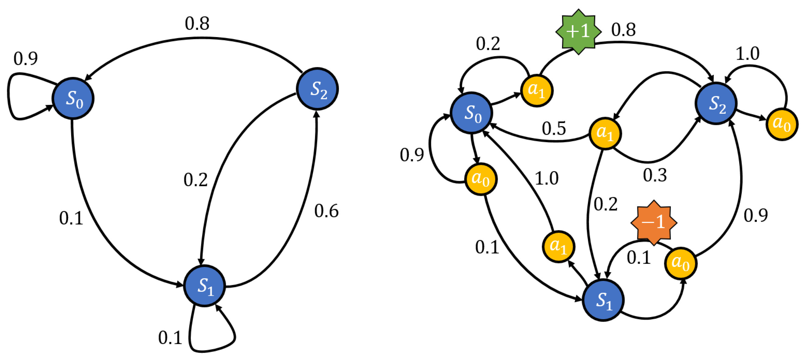
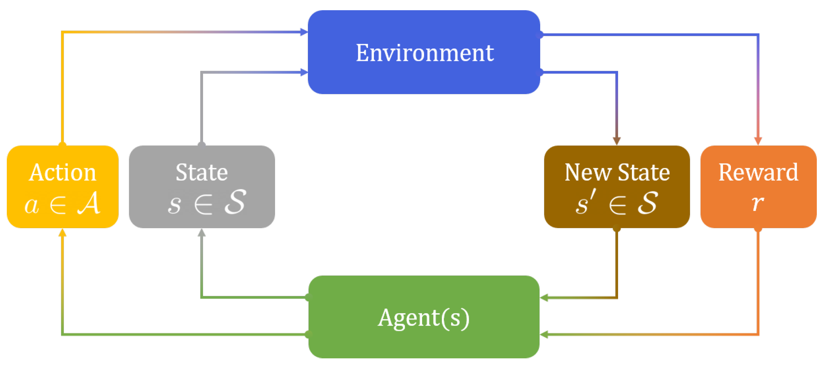
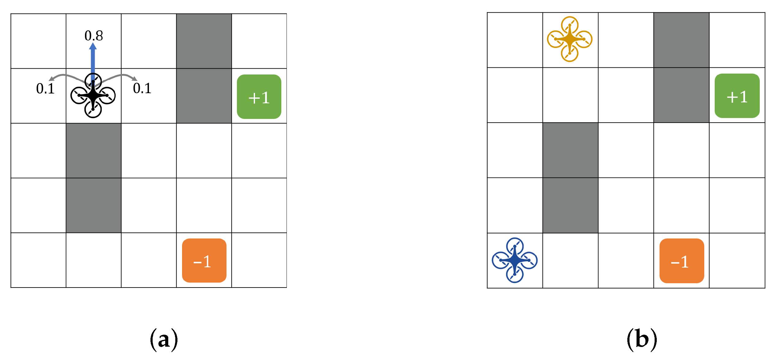
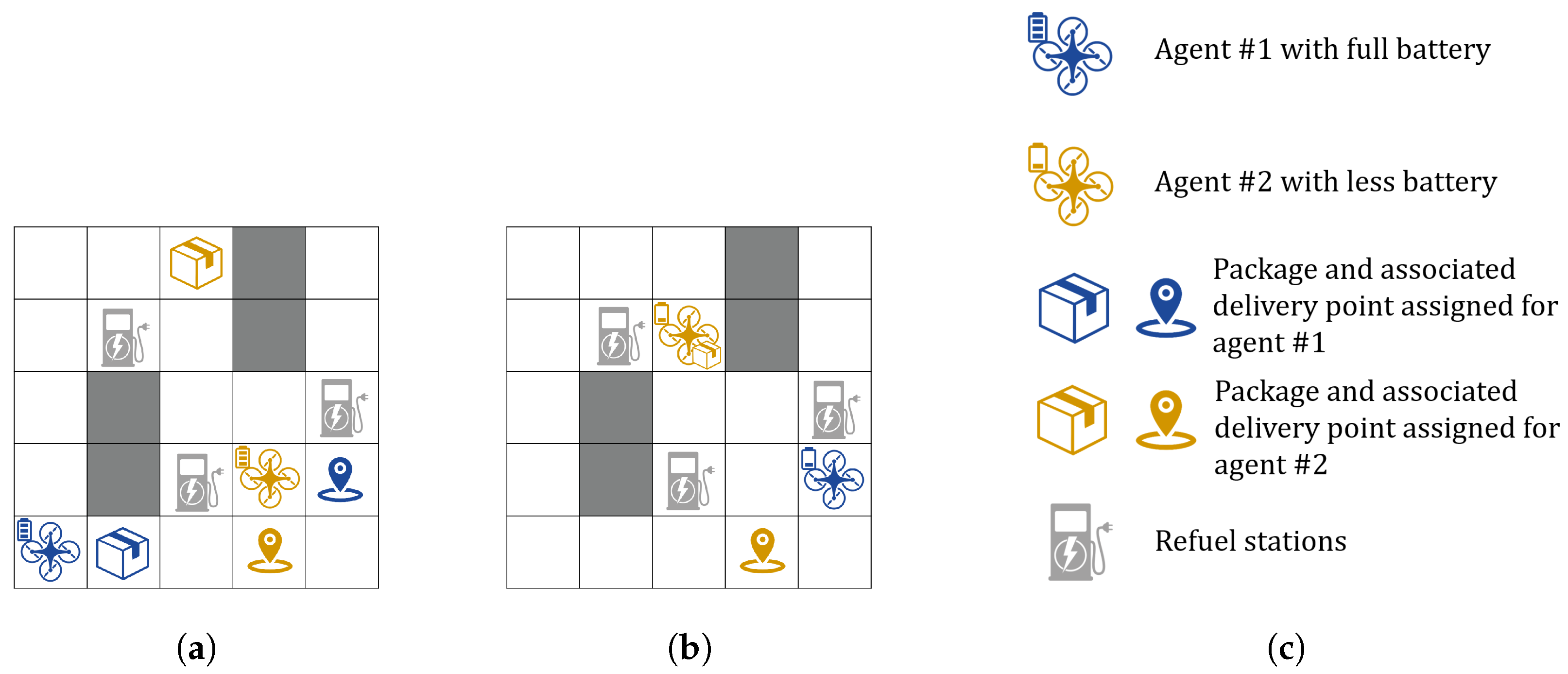
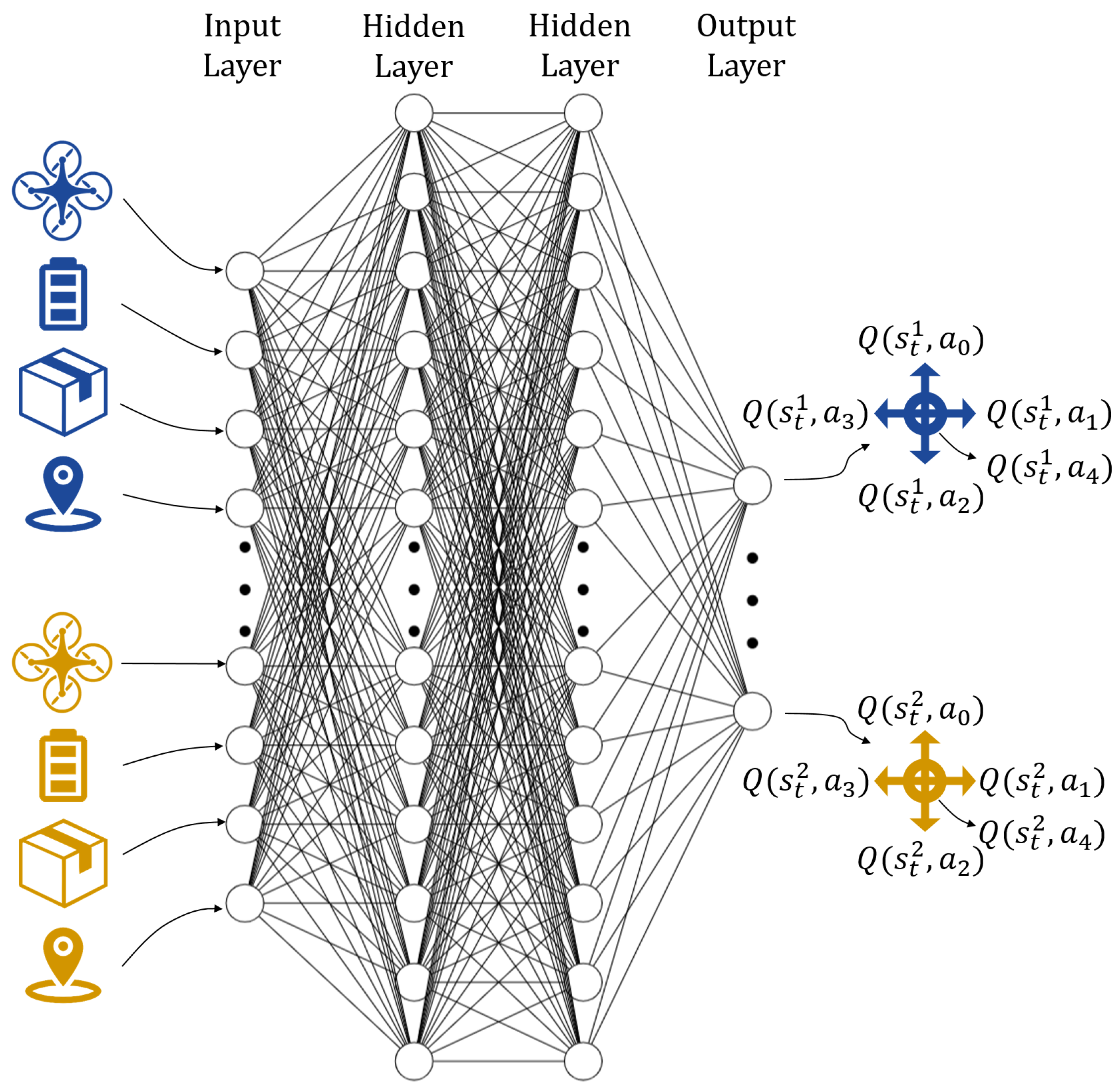
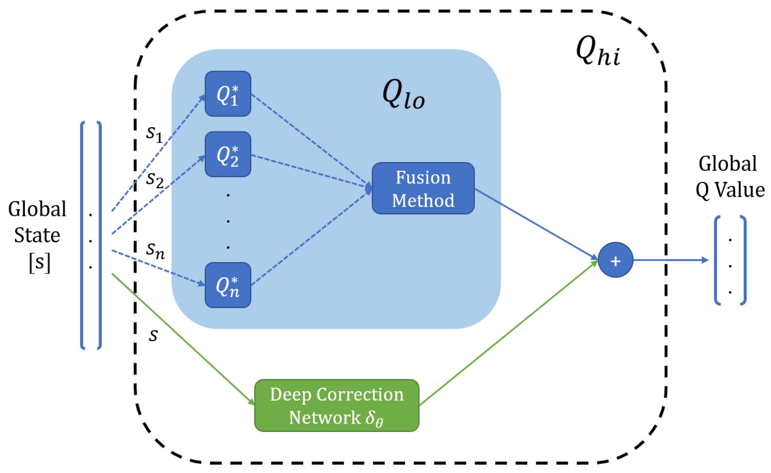
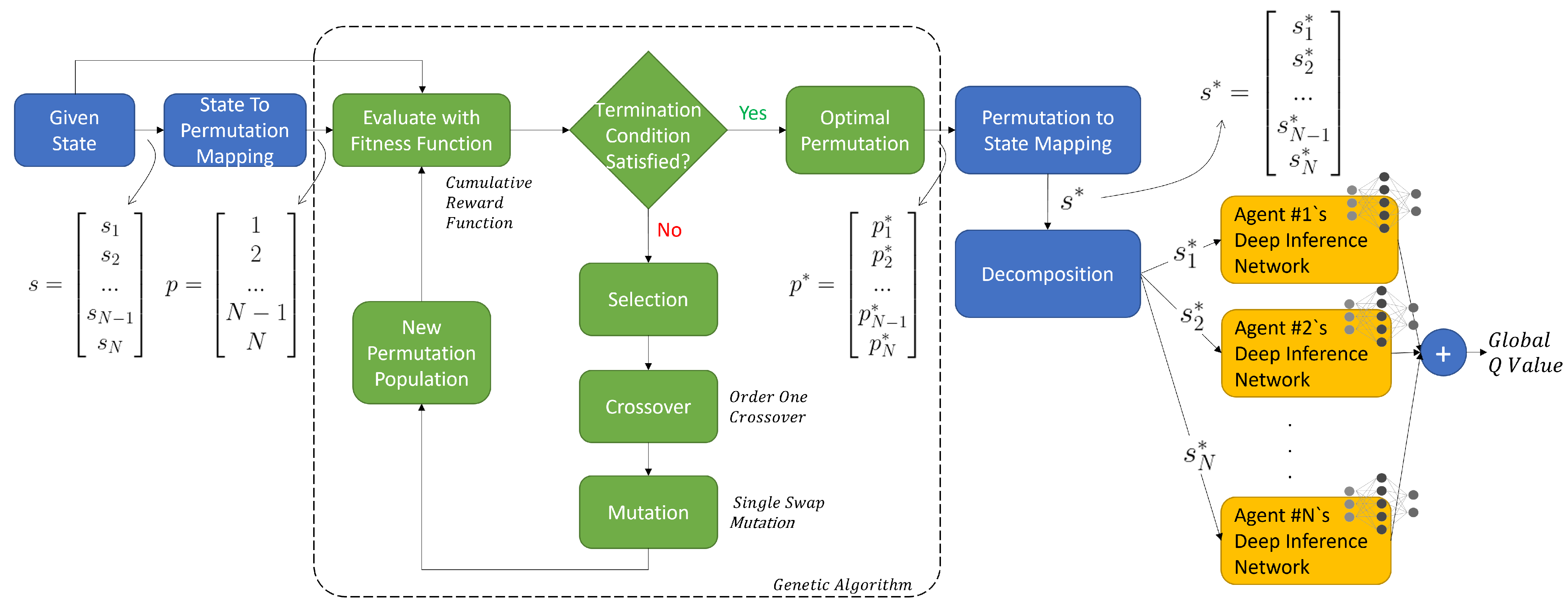
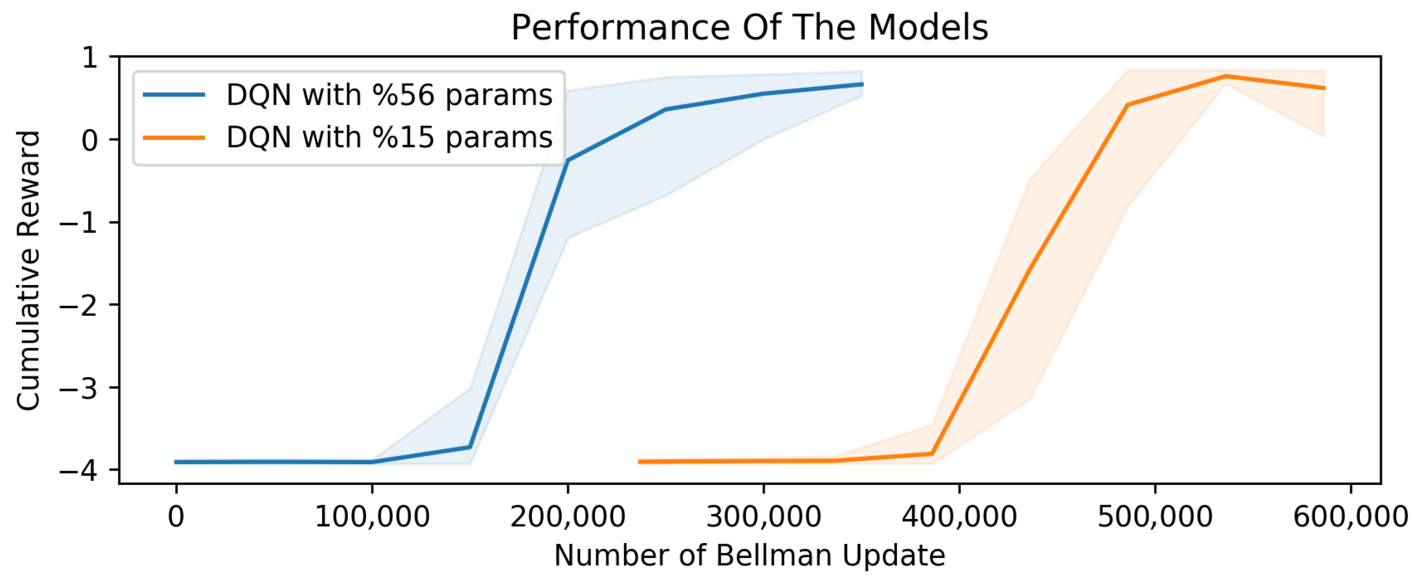


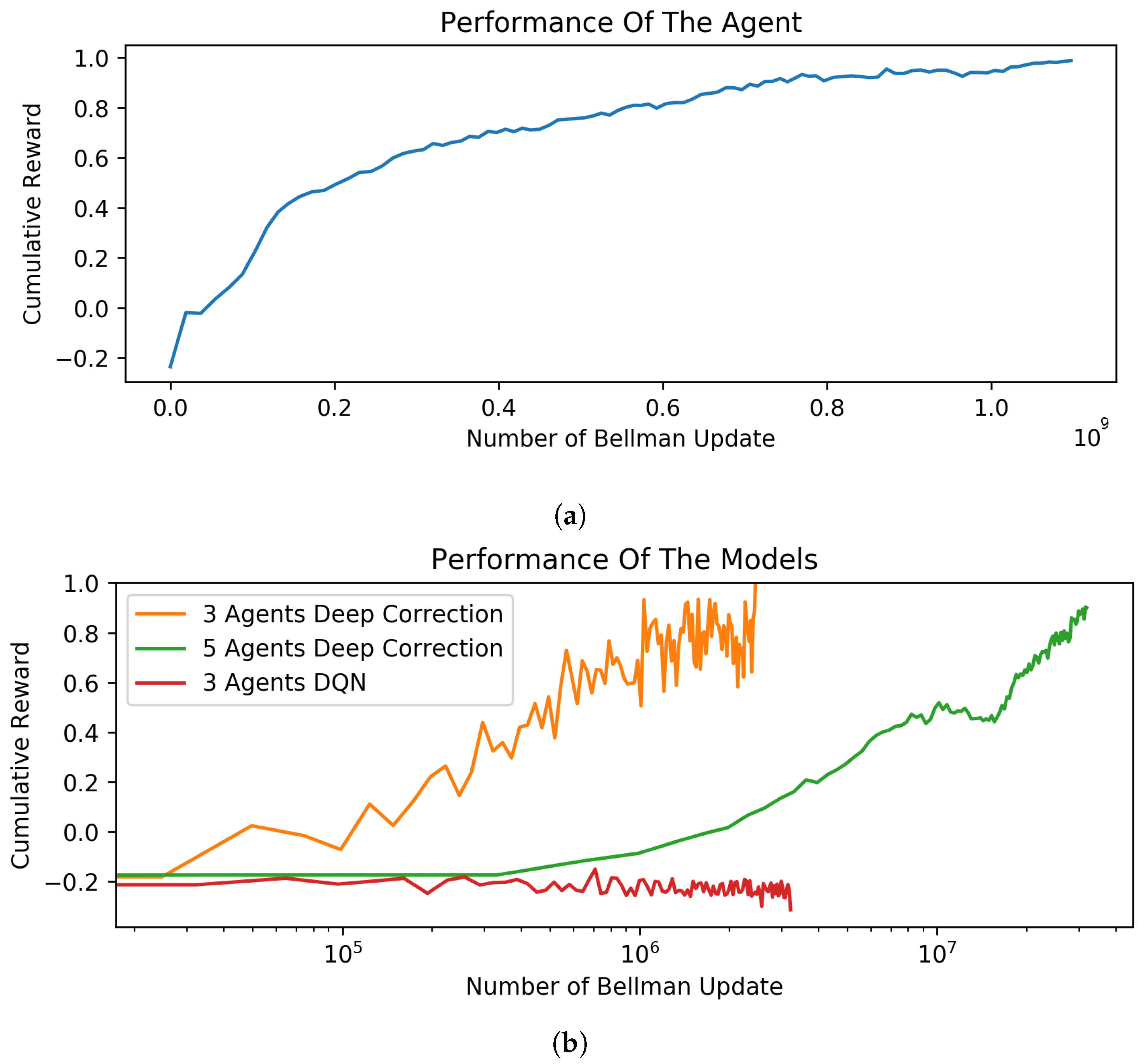
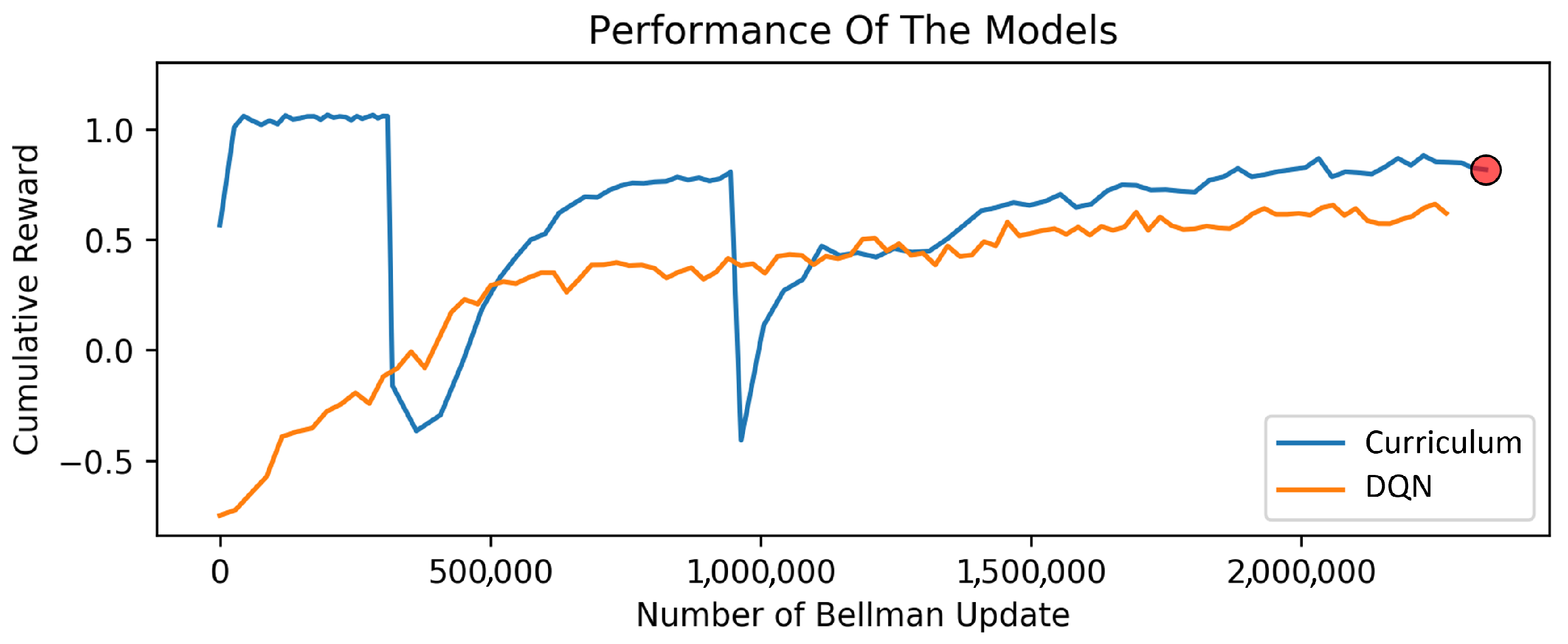
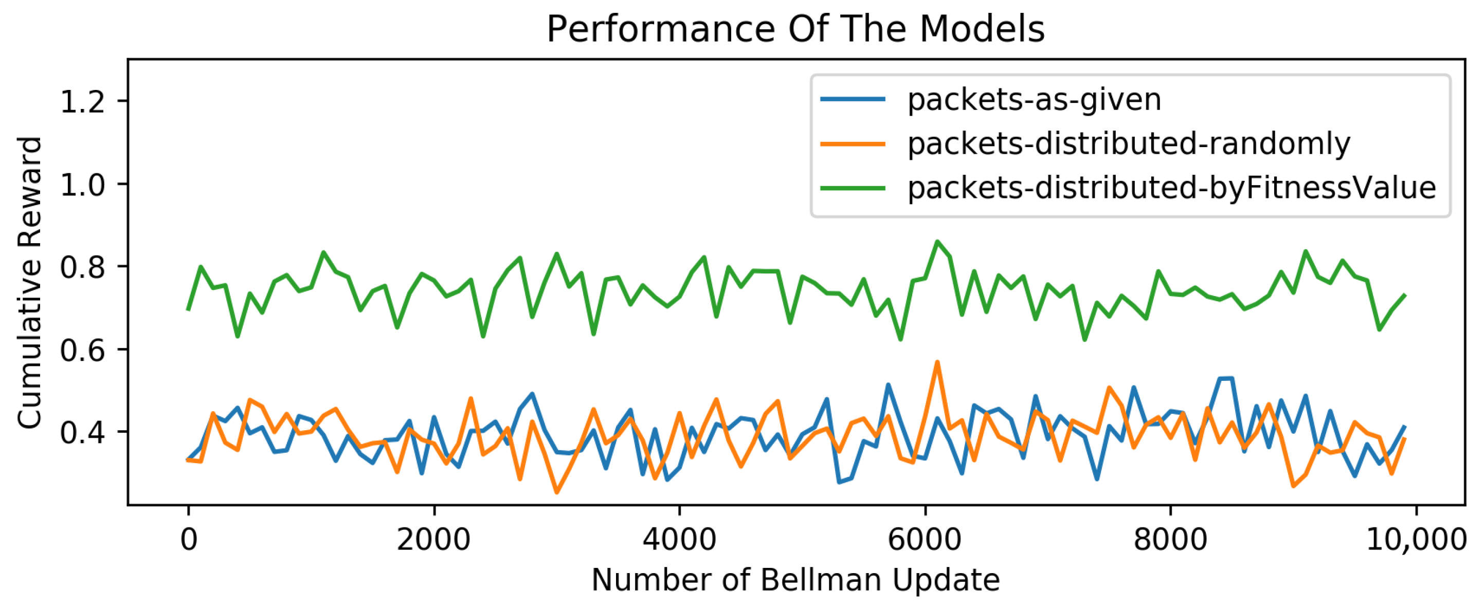
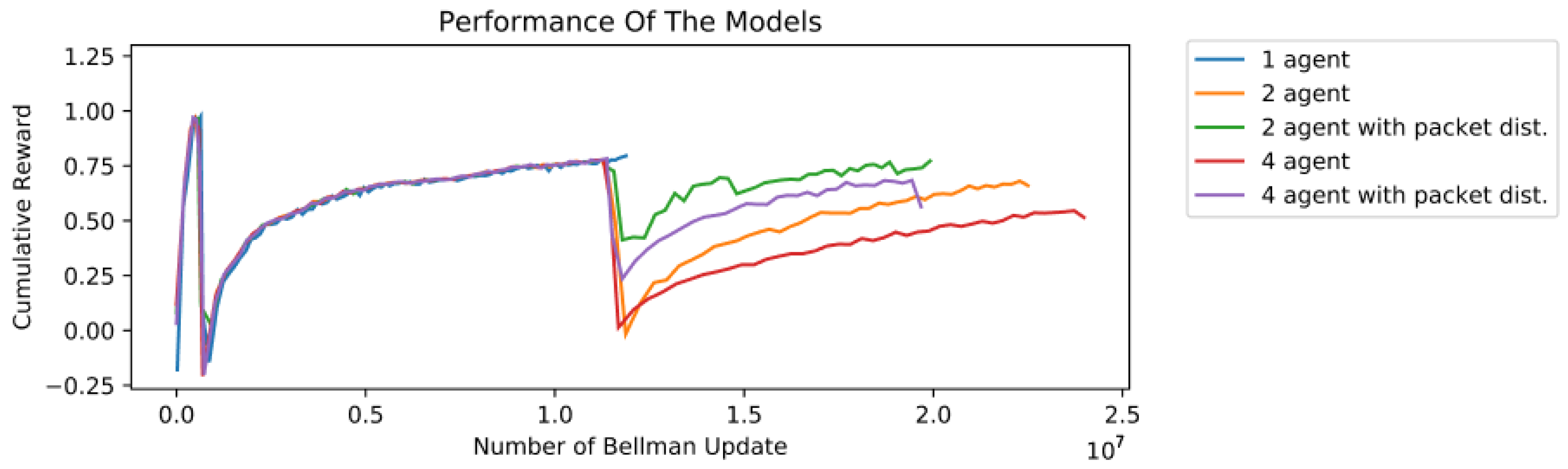
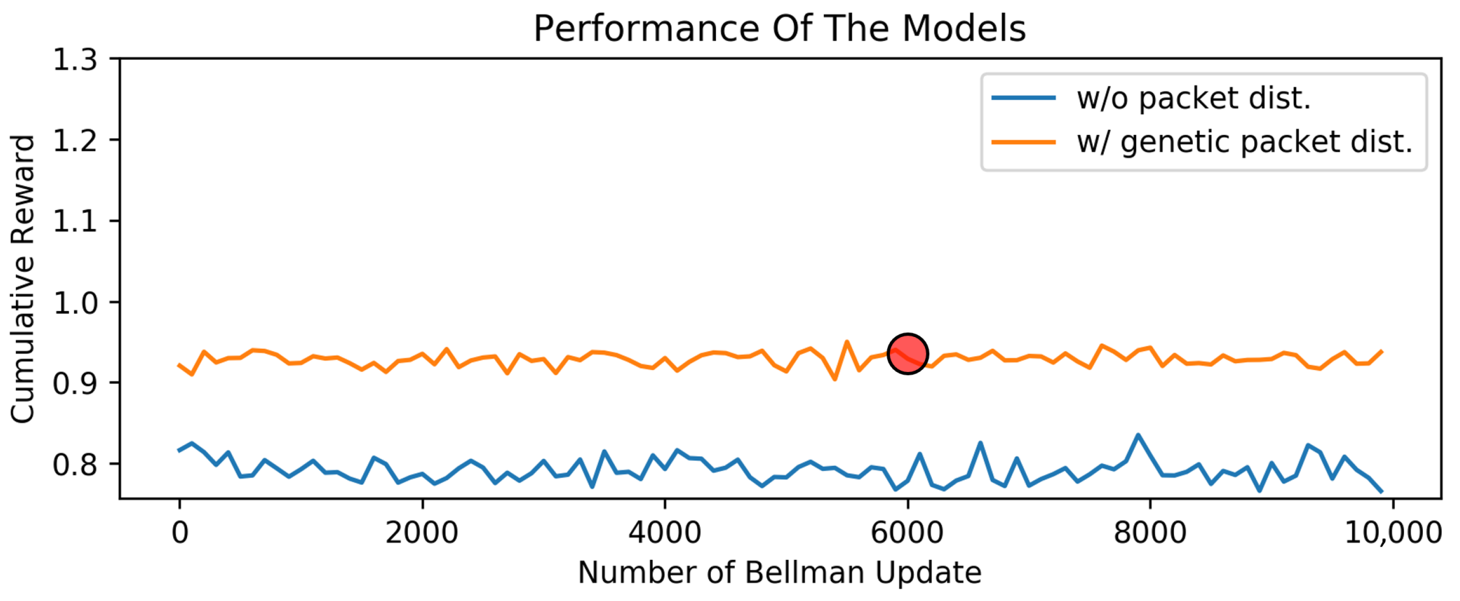
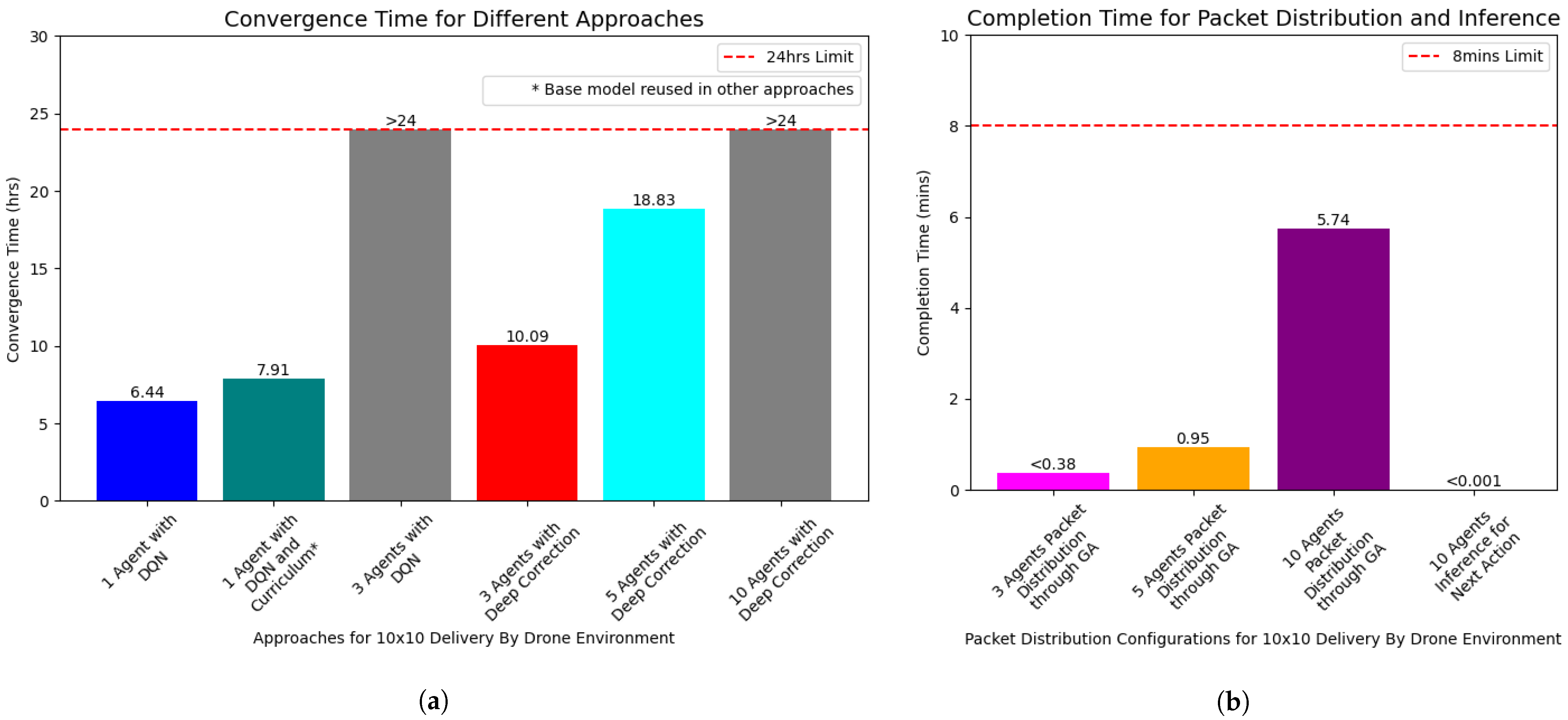
Disclaimer/Publisher’s Note: The statements, opinions and data contained in all publications are solely those of the individual author(s) and contributor(s) and not of MDPI and/or the editor(s). MDPI and/or the editor(s) disclaim responsibility for any injury to people or property resulting from any ideas, methods, instructions or products referred to in the content. |
© 2024 by the authors. Licensee MDPI, Basel, Switzerland. This article is an open access article distributed under the terms and conditions of the Creative Commons Attribution (CC BY) license (https://creativecommons.org/licenses/by/4.0/).