State-of-Charge Trajectory Planning for Low-Altitude Solar-Powered Convertible UAV by Driven Modes

Abstract

The conversion efficiency of solar energy and the capacity of energy storage batteries limit the development of low-altitude solar-powered aircrafts in the face of challenging meteorological phenomena in the lower atmosphere. In this paper, the energy planning problem of solar-power convertible unmanned aerial vehicles (SCUAVs) is studied, and a degressive state-of-charge (SOC) trajectory planning method with energy management strategy (EMS) is proposed. The SOC trajectory planning strategy is divided into four stages driven by three modes, which achieves the energy cycle of SCUAV’s long-endurance cruise and multiple hovers without the need to fully charge the battery SOC. The EMS is applied to control the output of solar cell/battery and power distribution for each stage according to three modes. A prediction model based on wavelet transform (WT), long short-term memory (LSTM) networks and autoregressive integrated moving average (ARIMA) is proposed for the weather forecast in the low altitude, where solar irradiance is used for the prediction of solar input power, and the wind and its inflow direction take into account the multi-mode power prediction. Numerical and simulation results indicate that the effectiveness of the proposed SOC trajectory planning method has a positive impact on low-altitude solar-powered aircrafts.

1. Introduction

Solar-powered UAVs have attracted worldwide attention due to their advantages such as environmental protection, zero fuel consumption, long endurance and low noise [1,2,3,4,5,6]. Low-altitude SCUAV is a type of electric UAV that combines the advantages of the solar-powered fixed-wing UAV and the rotorcraft, which can realize the task requirements of vertical takeoff and landing, long endurance and multiple hovers [7,8,9]. The development of the SCUAV will provide a more flexible and highly efficient unmanned flight platform because higher resolution imaging in aerial photogrammetry, protective detection and careful observation of wildlife, as well as its study, have theoretical significance and applicable value. However, challenging meteorological phenomena in low-altitude (cloud, wind, and other weather problems), weak energy systems, such as the low efficiencies of solar cells and insufficient battery capacities, dramatically limit the endurance and mission capability of the SCUAV. Therefore, energy planning, energy management and low-altitude meteorology forecast of the SCUAV in the multi-mode (rotor mode, transition mode and fixed-wing mode) are urgent challenges and core technologies that need to be solved.

The purpose of energy planning of the SCUAV is to achieve long endurance and complete the mission quickly. However, there is little information available on energy of low-altitude SCUAV. The existing studies mainly focused on high-altitude solar-powered fixed-wing UAVs, divided into two major areas. On the one hand, gravitational potential, wind shear and other methods are used as flight trajectory planning energy resources to reduce the weight of energy storage battery [10,11,12,13,14]. On the other hand, the UAVs increase solar income energy in the normal direction of the wing by adjusting attitude [15,16,17]. Moreover, these works, combining the altitude and wind shear with attitude trajectory planning optimizations, maximize the potential of energy. Gao et al. [13] investigated optimal flight trajectories for high-altitude long-endurance solar-powered UAVs coupled with the gravitational potential energy and wind shear energy. Hosseini et al. [18] maximized battery energy using the altitude and attitude change to store and plan more energy. Ma et al. [19] carried out the optimization of flight trajectory planning and three-dimensional tracking based on gravity energy storage. Ni et al. [20] and Xi et al. [21] used the reinforcement learning method to optimize the flight trajectory and improve the energy management capability of a solar-powered aircraft to enhance long endurance performance. However, these studies are very constructive on high-altitude long-endurance fixed-wing solar-powered UAVs; the influence of low-altitude meteorological environment on the fixed-wing mode of UAV is not considered, as well as the energy planning in rotor and transition modes of the SCUAV.

EMSs play a key role in trajectory planning for solar-powered UAVs due to the unpredictability of solar energy, the lower specific capacity of energy storage batteries and the operation of solar-powered UAV. Numerous researchers have worked to maximize the potential of energy, adequate distribution of power from the solar cells and the power storage system to the motor and on-board systems in a healthy and efficient way [22,23]. Gao et al. [13,24] used EMS to store solar energy in gravitational potential to achieve a high-altitude long-endurance flight, showing that energy storage in altitude is one of the most efficient types of storage. Similar to Gao et al.’s work, Sun et al. [25] considered the EMS for high-altitude solar-powered UAVs in multiple flight phases which is more suitable for the day and night cycle flight in engineering applications. Hosseini et al. [18] developed power allocation on energy optimal in trajectory planning for hybrid powered UAVs, while Wang et al. [26] proposed a comprehensive energy optimal control strategy for mission profiles, which could realize the uninterrupted and stable power supply in the multiflight phase. Qi [27] studied an adaptive rule-based EMS to extend the battery lifetime, the strategy is adaptive with load conditions of power consumption variation. Wang Hui et al. [28] proposed an intelligent energy management for solar-powered UAVs, which considered details of a complex energy flow model and analyzed complex factors on energy distribution and flight trajectories. Cao et al. [9] proposed a complementary energy strategy to electric-powered CUAVs, the strategy used to guide the conceptual design of the SCUAV. Most of these strategies are suitable for high-altitude lower-discharge rate aircrafts; however, the batteries have a much shorter discharge time, and higher continuous discharge power and peak discharge power of low-altitude SCUAV are not taken into account.

The low-altitude meteorological environment seriously affects the power and energy balance of the SCUAV because of the decrease in the energy input and increase in power demand, where the most prominent parameters are solar irradiance and wind [3]. In recent years, the prediction research of the two has mainly been focused on smart grid and other applications [29,30]. A number of methods have been proposed to forecast solar irradiance, including persistence [31], classical statistical methods [32], machine learning [33], cloud motion tracking [34], numerical weather prediction [35], and hybrid models [36,37,38]. The hybrid prediction method is the most promising method for the solar irradiation prediction, which combines two or more methodologies to improve the advantages and accuracy while avoiding the drawbacks. However, there is little information available on SCUAV by the hybrid solar irradiance prediction model; its accurate prediction is advantageous for energy management and mission planning. For wind prediction, numerous studies have been undertaken on prediction models, including persistence [39], classical statistical [40] and hybrid model forecasting [41,42]. The hybrid prediction method improves on the historical data method’s shortcomings to account for the influence of future atmospheric movement and other factors, as well as the single numerical weather forecast’s lack of accurate description of the target area due to the influence of model, time, and topographic space. The prediction of wind speed has a significant impact on the output power, which has crucial implications for the SCUAV in a low altitude.

In this work, we solve the problem of high-efficient flight of the low-altitude SCUAV from energy trajectory planning. The primary contributions of this paper are summarized as follows: (1) A degressive SOC trajectory planning method with multiobjective optimizaion is proposed for SCUAV driven by the multi-mode. (2) A degressive energy management strategy with meteorological phenomena is proposed to the management and distribution of power for the multi-mode of SCUAV. (3) A WT-LSTM-ARIMA hybrid prediction model is explored to solve the problem of short-time prediction of low-altitude weather. (4) A multi-mode power model considering the direction of the flow velocity is developed for convertible UAV.

The detailed layout of this paper is presented as follows: Section 2 establishes a system model of SCUAV. A SOC trajectory planning strategy with EMS is proposed in Section 3. Section 4 presents simulation results and performance discussions. Finally, conclusions are summarized in Section 5.

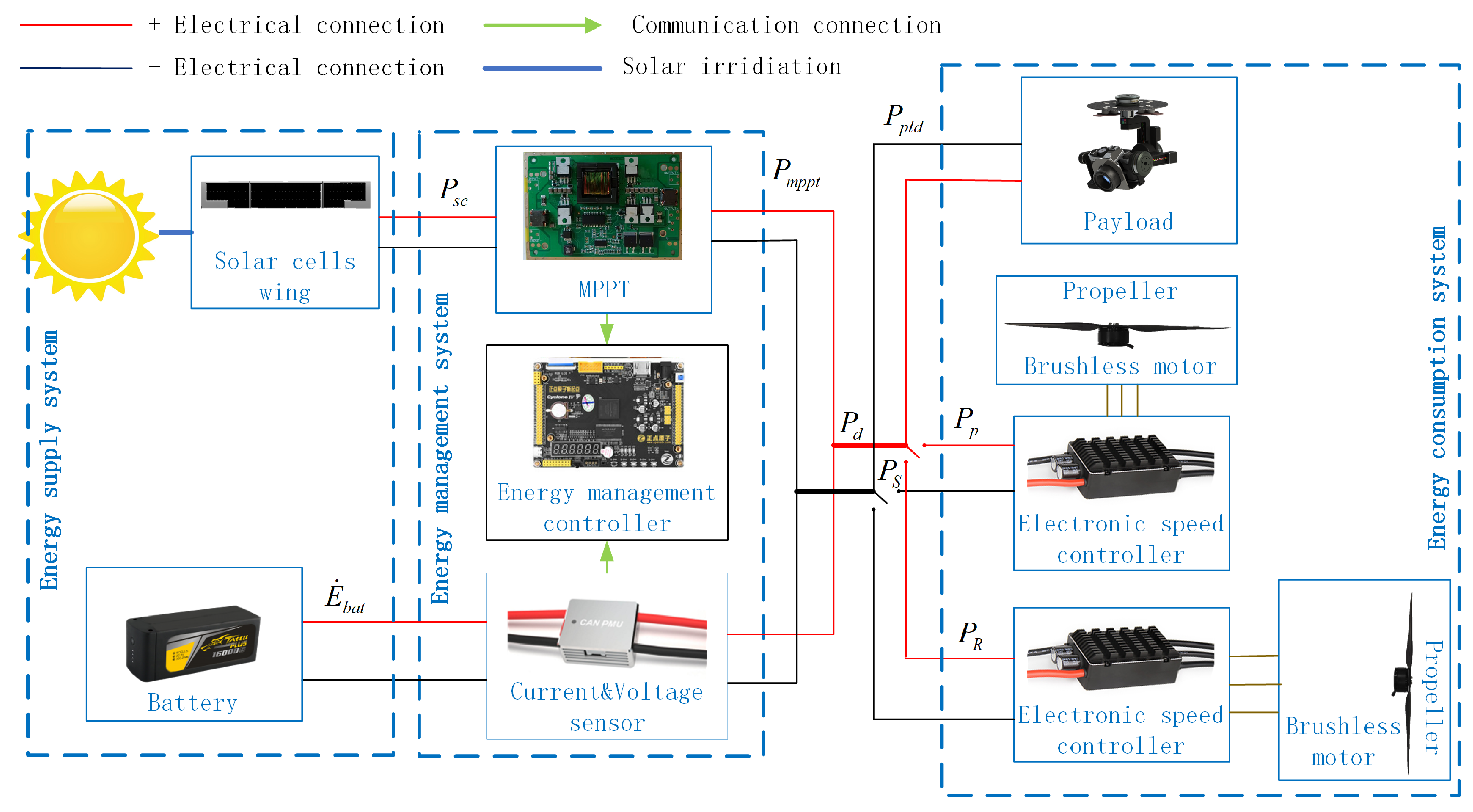
2. System Description and System Model

In this section, the system description of the SCUAV is presented and a typical mission profile is established. Moreover, a typical topology of a hybrid solar cell/battery is introduced, and the energy flow of a hybrid energy system is analyzed. On this basis, the mathematical model is established, including a multi-mode power model, a solar income model and an energy storage model.

2.1. System Description

The SCUAV has the characteristics of complex application scenarios, various tasks, long endurance and multiple hovers. Therefore, the mission profile of the SCUAV refers to the flight mode in which the various stages of the UAV mission appear and describes the flight of the plane mission. Based on the mission profile of the SCUAV, this paper formulates a SOC trajectory planning strategy using energy management. Aiming at multiple hovers and cruises, which are the characteristic tasks of the SCUAV, a flight mission profile is designed, including the vertical takeoff stage, the transition stage, the multiple cruises stage, the multiple hovers stage and the vertical landing stage. The specific mission profile over the day is shown in Figure 1, which contains the appearance order of the flight mode in each stage (top) and the schematic curve corresponding to the P-t of each flight mode in each stage (lower).

Each flight mode and phase are described as follows.

(1)

Vertical Takeoff Phase: It is assumed that the SCUAVs take off vertically on the horizontal ground and climb to a safety altitude h at a fixed climbing velocity in the vertical direction. The whole vertical takeoff process is in the rotor mode, and the onboard power P of the system is larger because the axial thrust needs to be generated to overcome the gravity of the SCUAV.

(2)

Transition Phase: At this phase, it is assumed that the SCUAVs transform the axis direction of the power system by a mechanism to achieve the transition between the rotor mode and the fixed-wing mode. During the transition phase, the onboard power of the system is decreased in the process of the conversion from the rotor to the fixed-wing mode, while the required power of the system is increased during the cruise-to-hover transition.

(3)

Multiple Hovers Phase: The SCUAV assumes that the entire process is to convert its mechanism towards the vertical direction to provide the aircraft to the hovering mission. The multiple hovers process is in the rotor mode, and the required power of the system is smaller than that of the vertical takeoff stage.

(4)

Multiple Cruises Phase: The SCUAV assumes that the whole process is flying at a speed of maximum range/maximum endurance in the fixed-wing mode. During the multiple cruises phase, the required power of the SCUAV is lowest, the solar module absorbs solar irradiance and converts it into electricity, some of which is used for cruise missions, while the remaining energy is used to charge the battery.

The modes transform, and energy interactions in the (2), (3) and (4) stages of multiple cycles are carried out, realizing multiple hovers and the long-endurance level flight of the SCUAV. In the multi-mode cycle stages (Figure 1 lower), the power and energy balance of the SCUAV is affected by challenging external meteorological phenomena in a low altitude (clouds, wind) as well as internal solar irradiance law. These factors can be summarized into two types—energy input reduction and power demand increase.

(a)

Input energy decrease by solar irradiation. Due to solar radiation intensity changes caused by external (temperature, humidity, weather) and internal factors (days, time), the absorbed energy of the SCUAV decreases.

(b)

Output power increase by wind disturbance. The complex speed and direction of wind increase the thrust and drive power in multiple modes, resulting in an increase in the required power.

(5)

Vertical Landing Phase: During the vertical landing phase, the SCUAV is transformed to achieve thrust in the vertical direction until it lands on the ground. At this phase, the onboard power of the system is lower than that of the vertical takeoff phase.

2.2. Operation Condition Analysis

The energy system of the SCUAV, as a system for energy generation, storage, conversion, regulation and distribution, ensures the uninterrupted energy supply for the required multi-modes and payload, and realizes the cyclic flow of energy consumption and generation. The typical topology of a hybrid energy system is demonstrated in Figure 2.

The topology includes the energy supply system, the energy management system and the energy consumption system. Specifically, it describes the energy conversion between solar, chemical storage and electric energy from the energy supply system, the energy management system to energy consumption by the energy flow. The energy flow adopts the power form to indirectly describe the change in the multi-phase flight profile and the multi-mode, and the entire power flow primarily comprises payload power $P_{pld}$, rotor mode power $P_R$, fixed-wing mode power $P_P$, transition mode power $P_S$, solar cell power $P_{sc}$, MPPT power $P_{mppt}$, and battery charging/discharging power ${\dot{E}}_{bat}$ printed on the right in Figure 2.

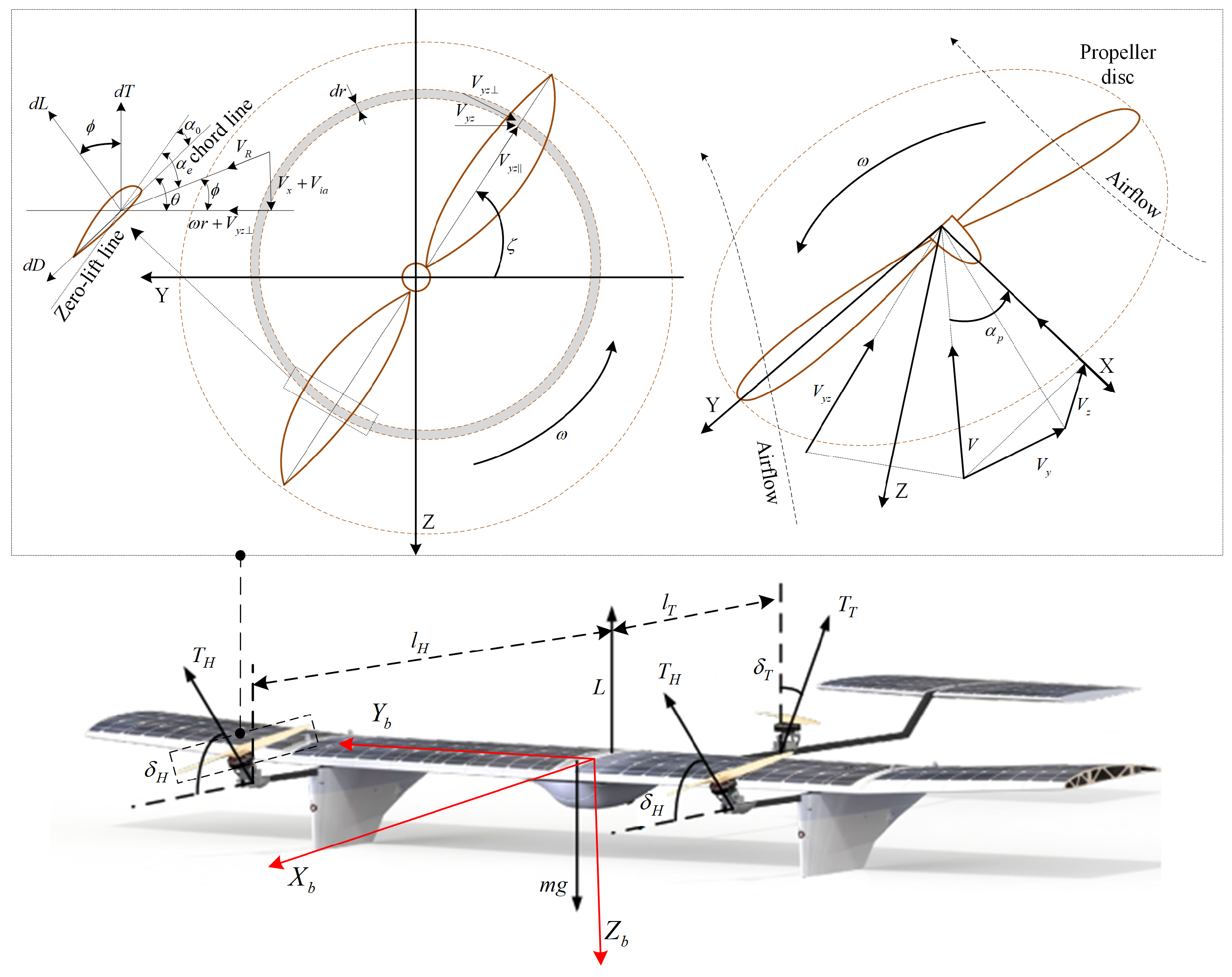
2.3. Multi-Mode Power Model

2.3.1. Propeller Aerodynamics

Blade Element Momentum Theory (BEMT), combining the blade element theory and the conservation of momentum, is widely used; it has relative precision and calculation efficiency. In this paper, we adopt BEMT to calculate the multi-mode thrust faced with a different angle of attack of the incoming flow and propeller-induced velocity [43]. The velocity and force acting on each blade element can be seen in Figure 3.

For a propeller, it is assumed that there is an annulus at $dr$ of the propeller, where differential thrust $dT$ can be obtained using momentum theory over a segment of the annulus. Thus, differential thrust $dT$ of an annulus can be expressed as

$$dT=2\rho r{\int }_{\zeta =0}^{2\pi }{V}_{ia}\sqrt{{(V_x+V_{ia})}^2+V_{yz}^2}d\zeta dr$$

(1)

where $\rho$ is air density, r is radial distance from the propeller rotation axis, $\zeta$ is the blade azimuth angle for the angular position of the propeller blade, $\omega$ is propeller angular velocity. $V_{ia}=V_{ia,0}(1+\frac{15\pi }{32}tan\left(\frac{\chi }{2}\right)\frac{r}{R}cos\zeta )$ is axial induced velocity, where $V_{ia,0}$ is the induced velocity at the center, R is propeller radius, $\chi =arctan\left[V_{yz}/(V_x+V_{ia,0})\right]$ is the wake skew angle, $V_{yz}=Vsin{\alpha }_p$ and $V_x=Vcos{\alpha }_p$ are the axial velocity along the propeller rotation axis and the in-plane velocity in propeller rotation, respectively. ${\alpha }_p$ is the incoming flow angle. $F=\frac{2}{\pi }arccos\left(e^{\frac{(r-R)K_b}{2rsin\varphi }}\right)$ is Prandtl’s tip loss factor, where $K_b$ is the number of propeller blades, $\varphi =arctan\left(\frac{V_x+V_{ia}}{\omega r+V_{yz\perp }}\right)$ is the flow angle at the tip, where $V_{yz\perp }=V_{yz}sin\zeta$ is perpendicular to the propeller blade while $V_{yz\Vert }$ is along propeller blade.

In blade element theory, differential thrust dT at differential element dr of the propeller blade at radial distance r from the propeller rotation axis is given as

$$dT=\frac{K_b}{4\pi }\rho c_b{\int }_{\zeta =0}^{2\pi }{V}_R^2\left(C_{l}cos\varphi -C_{d}sin\varphi \right)d\zeta dr$$

(2)

where $c_b$ is the chord length of each blade element $dr$. $C_l$ and $C_d$ are the lift and drag coefficients at the effective angle of attack ${\alpha }_e$ for differential lift dL and drag dD acting on the blade element. $V_R=\sqrt{{(V_x+V_{ia})}^2+{(\omega r+V_{yz\perp })}^2}$ is the resultant flow to each blade section. The induced velocity at the propeller disc is determined by simultaneous solution of Equations (1) and (2) using an iterative method for all annuli, and then the multi-mode thrust T is calculated.

2.3.2. Flight Dynamics

SCUAV, which consists of a fixed-wing mode, a rotor mode and a transition mode, have different required powers in flights of different modes. Supposing that the SCUAV has the usual plane of symmetry and flies with zero side-slip in wind gust conditions, the six-degree-of-freedom dynamic model is decoupled into lateral and longitudinal. Crosswind disturbances are ignored because they vary with time and are difficult to forecast, so in this paper we study flow disturbance and balance it by longitudinal control. As shown in Figure 3, the dynamic equation of SCUAV can be expressed as follows:

$$\left\{\begin{array}{c}{\displaystyle \frac{dV}{dt}=\frac{T_{H}cos(\alpha +{\delta }_H)-T_{T}cos{\delta }_{T}sin\alpha -D-mgsin\gamma -m{\dot{\omega }}_{w}cosrcos\psi }{m}}\hfill \\ {\displaystyle \frac{d\gamma }{dt}=\frac{\begin{array}{c}{T}_{H}sin(\alpha +{\delta }_H)cos\phi +T_{T}cos{\delta }_{T}cos\alpha cos\phi +Lcos\phi -mgcos\gamma +m{\dot{\omega }}_{w}sin\gamma cos\psi \hfill \end{array}}{mV}}\hfill \\ {\displaystyle \frac{d\psi }{dt}=\frac{T_{H}sin(\alpha +{\delta }_H)sin\phi +T_{T}sin{\delta }_{T}cos\alpha sin\phi +Lsin\phi -m{\dot{\omega }}_{w}sin\psi }{mVcos\gamma }}\hfill \\ {\displaystyle \frac{d{\omega }_z}{dt}=\frac{M_z+T_T{l}_T+T_{H}cos(\alpha +{\delta }_H)l_H}{J_z}}\hfill \\ {\displaystyle \frac{dx}{dt}=Vcos\gamma cos\psi +{\omega }_w}\hfill \\ {\displaystyle \frac{dy}{dt}=Vcos\gamma sin\psi }\hfill \\ {\displaystyle \frac{dh}{dt}=Vsin\gamma }\hfill \\ {\displaystyle \frac{d\theta }{dt}={\omega }_z}\hfill \\ \theta =\alpha +\gamma \hfill \end{array}\right.$$

(3)

where $T_H$, $T_T$, L, D, m represent aircraft head motor thrust, tail motor thrust, lift force, drag force and mass, respectively. V, $\gamma$, $\psi$, ${\omega }_w$, $\alpha$, $\theta$ and $\phi$ represent airspeed, track angle, heading angle, wind speed, attack angle and roll angle, respectively. ${\delta }_H$ and ${\delta }_T$ are the deflection angles of the head and tail motor. $l_H$ and $l_T$ are the pitch levers for head and tail motor thrust. ${\omega }_z$ is pitch angle velocity. $J_z$ is the pitch moment of inertia.

Generally, the flight aerodynamic forces and the moment acting on the SCUAV can be calculated with the following formula:

$$\left\{\begin{array}{c}D=\frac{1}{2}\rho V{S}_w{C}_d\hfill \\ L=\frac{1}{2}\rho V{S}_w{C}_l\hfill \\ M_z=\frac{1}{2}\rho V{S}_w{c}_w{C}_m\hfill \end{array}\right.$$

(4)

where $S_w$, $c_w$ and $C_m$ are the wing area, the mean aerodynamic chord and the coefficient of the pitching moment.

Typical fixed-wing flight conditions include cruising, climbing, descending, etc. In this mode, a classical six-degree-of-freedom point mass dynamical model can be uniformly described using the following formula:

$$\left\{\begin{array}{c}{\displaystyle \frac{dV}{dt}=\frac{T_{H}cos\left(\alpha \right)-D-mgsin\gamma -m{\dot{\omega }}_{w}cosrcos\psi }{m}}\hfill \\ {\displaystyle \frac{d\gamma }{dt}=\frac{T_{H}sin\left(\alpha \right)cos\phi +Lcos\phi -mgcos\gamma +m{\dot{\omega }}_{w}sin\gamma cos\psi }{mV}}\hfill \\ {\displaystyle \frac{d\psi }{dt}=\frac{T_{H}sin\left(\alpha \right)sin\phi +Lsin\phi -m{\dot{\omega }}_{w}sin\psi }{mVcos\gamma }}\hfill \\ {\displaystyle \frac{dx}{dt}=Vcos\gamma cos\psi +{\omega }_w}\hfill \\ {\displaystyle \frac{dy}{dt}=Vcos\gamma sin\psi }\hfill \\ {\displaystyle \frac{dh}{dt}=Vsin\gamma }\hfill \\ {\displaystyle \frac{d{\omega }_z}{dt}=\frac{M_z}{J_z}}\hfill \\ {\displaystyle \frac{d\theta }{dt}={\omega }_z}\hfill \\ \theta =\alpha +\gamma \hfill \end{array}\right.$$

(5)

Typical rotor flight conditions include vertical ascent, hover, vertical descent, etc. When operating in this mode, a longitudinal three-degree-of-freedom dynamic model is established as follows:

$$\left\{\begin{array}{c}{\displaystyle \frac{dV}{dt}=\frac{-T_{H}sin\left(\alpha \right)-T_{T}cos{\delta }_{T}sin\alpha -D-mgsin\gamma -m{\dot{\omega }}_{w}cosr}{m}}\hfill \\ {\displaystyle \frac{d\gamma }{dt}=\frac{T_{H}cos\left(\alpha \right)+T_{T}cos{\delta }_{T}cos\alpha +L-mgcos\gamma +m{\dot{\omega }}_{w}sin\gamma }{mV}}\hfill \\ {\displaystyle \frac{d{\omega }_z}{dt}=\frac{T_T{l}_T-T_{H}cos(\alpha +{\delta }_H)l_H}{J_z}}\hfill \\ {\displaystyle \frac{dx}{dt}=Vcos\gamma +{\omega }_w}\hfill \\ {\displaystyle \frac{dh}{dt}=Vsin\gamma }\hfill \\ {\displaystyle \frac{d\theta }{dt}={\omega }_z}\hfill \\ \theta =\alpha +\gamma \hfill \end{array}\right.$$

(6)

Flight conditions in the transition mode are complex between the rotor mode and the fixed-wing mode, but the duration is relatively short. Pitch control is mainly used for trimming the process of transformation, especially the rotor moment. This article adopts a tilting scheme which is a fixed altitude transition. In the conversion process, coordination between forward flight speed and tilting angle is required to achieve the transition mode. According to this, the longitudinal three-degree-of-freedom dynamic model of the transition mode can be expressed as follows:

$$\left\{\begin{array}{c}{\displaystyle \frac{dV}{dt}=\frac{T_{H}cos(\alpha +{\delta }_H)-T_{T}cos{\delta }_{T}sin\alpha -D-m{\dot{\omega }}_w}{m}}\hfill \\ {\displaystyle \frac{d\gamma }{dt}=\frac{T_{H}sin(\alpha +{\delta }_H)+T_{T}cos{\delta }_{T}cos\alpha +L-mg}{mV}}\hfill \\ {\displaystyle \frac{d{\omega }_z}{dt}=\frac{M_z-T_T{l}_T+T_{H}cos(\alpha +{\delta }_H)l_H}{J_z}}\hfill \\ {\displaystyle \frac{dx}{dt}=V+{\omega }_w}\hfill \\ {\displaystyle \frac{dh}{dt}=0}\hfill \\ {\displaystyle \frac{d\theta }{dt}={\omega }_z}\hfill \\ \theta =\alpha +\gamma \hfill \end{array}\right.$$

(7)

2.3.3. Power Model

A static model is established based on force balance and moment balance for the multi-mode power system considering their working efficiency. Specifically, in the rotor mode, the power of the propulsion system mainly comes from the hovering, vertical induced velocity, and forward and backward flight velocity. In the transition mode, the power of the drive system is based on the total sum of the forward flight speed and the axial induced speed of the tilting motor. In the fixed-wing mode, the power of the dynamic is generated by the flight overcoming drag. The required power for the multi-mode power system based on horizontal and vertical directions can be calculated as follows [44]:

$$\left\{\begin{array}{c}{\displaystyle P_R=\frac{(T_H+T_T)V_{i}cos\alpha +(T_H+T_T)Vsin\alpha }{{\eta }_p}}\hfill \\ {\displaystyle P_S=\frac{\left[T_{H}sin(\alpha +{\delta }_H)+T_{T}cos\alpha \right]V_i+T_{H}cos(\alpha +{\delta }_H)V}{{\eta }_p}}\hfill \\ {\displaystyle P_P=\frac{T_{h}V}{{\eta }_p}}\hfill \end{array}\right.$$

(8)

where $V_i=\left\{{\left[{(V·sin\gamma )}^2+4{V_h}^2\right]}^{0.5}-V·sin\gamma \right\}$ is the induced velocity for the axial climb, $V_h={\left[(T_H+T_L)cosa/\left(2\rho K_b{S}_R\right)\right]}^{0.5}$ is the axial rotor-induced velocity when $\gamma$ is equal to zero, where $S_R$ is the single disk area. ${\eta }_p$ denotes the working efficiency of the power system.

2.4. Solar Income Model

A simplified model for solar input power can receive solar irradiance by wing-covered solar cells and convert it into electric power, part of which is utilized for flight and the remainder to charge the battery. A typical mathematical model for the instantaneously collected solar radiation is as follows:

$$P_{sc}\left(t\right)=I\left(t\right)·S_{sc}·{\overrightarrow{\eta }}_{sm}·{\eta }_{sc}$$

(9)

where $I\left(t\right)$ is the solar radiation on a unit (1 m²) area as a function of a climatope. Solar module area $S_{sc}={\eta }_{co}{S}_w$, where ${\eta }_{co}$ is a coefficient of wing area $S_w$, is assumed to be covered by solar module area $S_{sc}$. ${\overrightarrow{\eta }}_{sm}$, denotes the solar module normal vector which describes the solar income direction from the aircraft body to the inertial reference frame [45]. Solar cell efficiency ${\eta }_{sc}={\eta }_{sm}.{\eta }_{cl}$ includes plate efficiency and wing camber efficiency.

2.5. Energy Storage Model

The state dynamic must be specified for the battery in terms of capacity and charging/discharging power for two time horizons. The battery SOC is a crucial metric for battery control. Considering charging and discharging efficiencies, the discrete-time SOC difference equation of the battery can be presented as follows [46]:

$$SOC(t+\Delta t)=\left\{\begin{array}{c}SOC\left(t\right)-\frac{1}{E_{bat,max}}\underset{t}{\overset{t+\Delta t}{\int }}{\dot{E}}_{bat}^{dchrg}(\Delta t)·{\eta }_{bat}dt,{\dot{E}}_{bat}(\Delta t)\le 0\hfill \\ SOC\left(t\right)-\frac{1}{E_{bat,max}}\underset{t}{\overset{t+\Delta t}{\int }}\frac{{\dot{E}}_{bat}^{chrg}(\Delta t)dt}{{\eta }_{bat}},{\dot{E}}_{bat}(\Delta t)>0\hfill \end{array}\right.$$

(10)

where $E_{bat,max}$ and ${\eta }_{bat}$ denote the maximum capacity of the battery and charging/discharging efficiency, respectively. ${\dot{E}}_{bat}^{chrg}\left(t\right)$ and ${\dot{E}}_{bat}^{dchrg}\left(t\right)$ denote the charging and discharging powers of the battery, respectively.

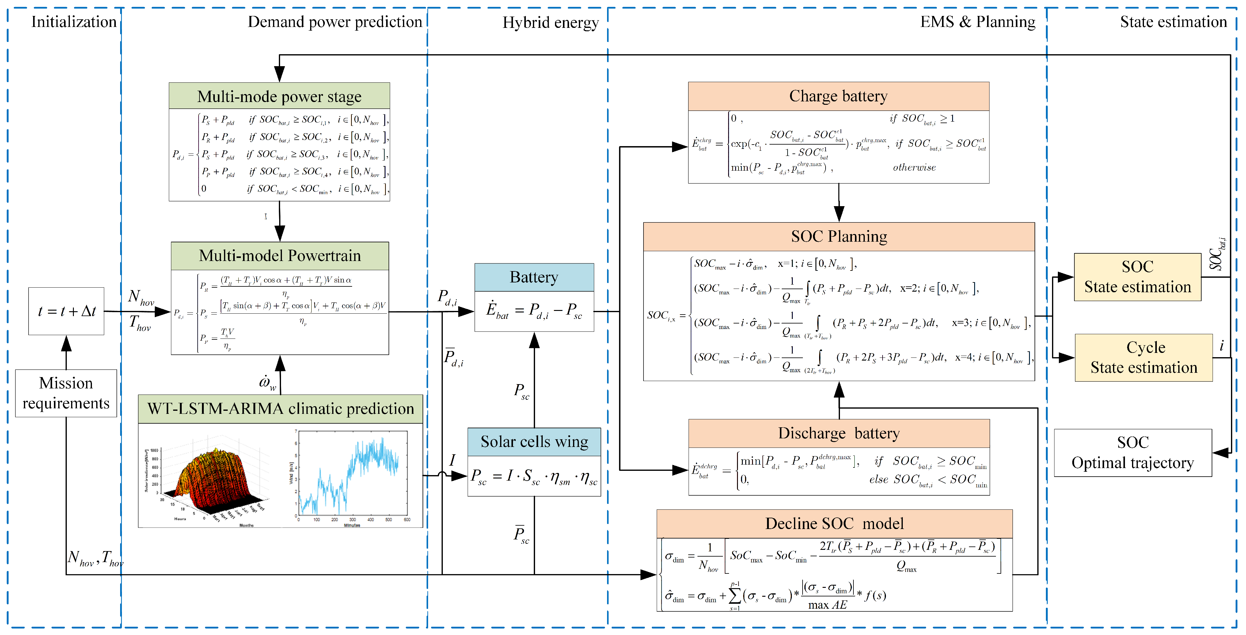
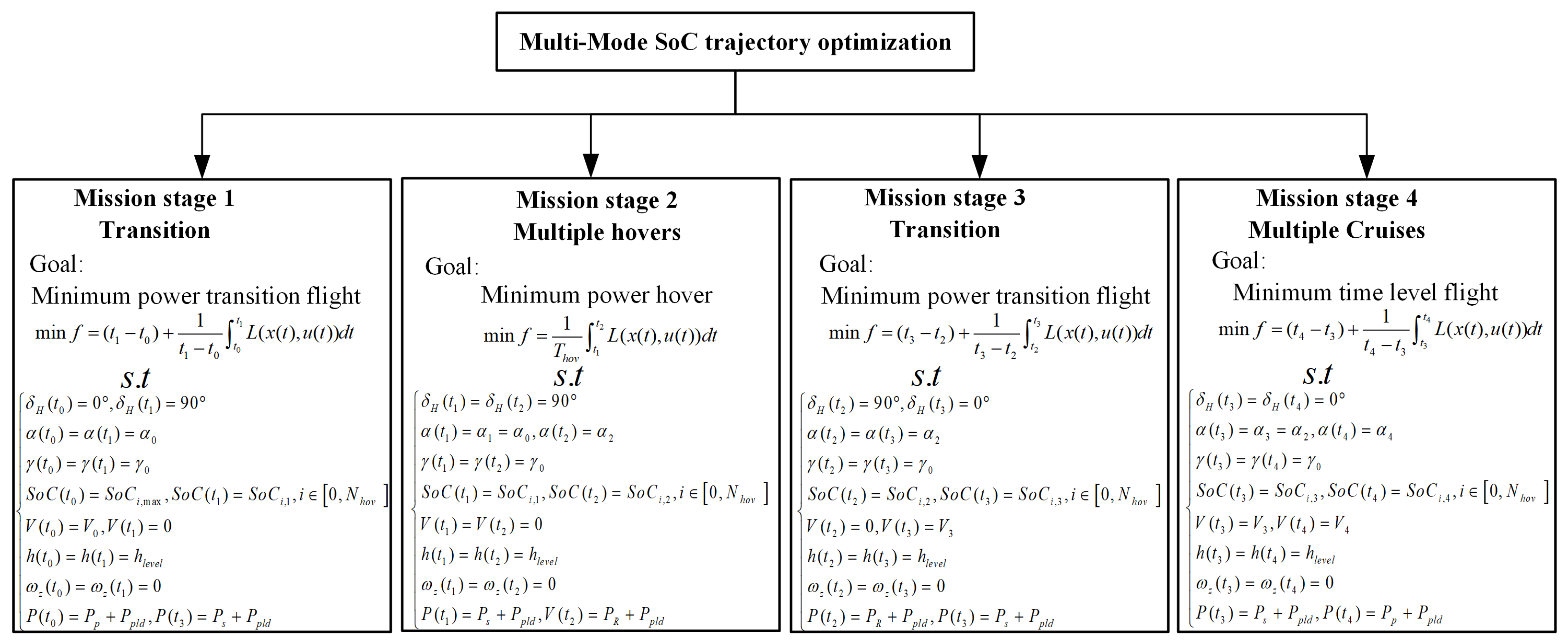
3. Degressive SOC Trajectory Planning Method

SOC trajectory planning plays an important role of the SCUAV in multiple hovers and long-endurance level flight. First, in order to achieve continuous stability of the flight profile, the properties of peak discharge power and safe charge/discharge, as well as the hybrid solar cell/battery can be managed reasonably and efficiently according to different power demands under different flight modes. An energy management strategy for multi-mode mission profile is proposed in this section. Second, a WT-LSTM-ARIMA prediction model for complex meteorological environment (solar irradiance, wind) in a low altitude is studied, which more accurately predicts demand power and solar power. Finally, a decreasing SOC trajectoty planning with multiobjective optimization is explored to maximize the use of energy and quickly complete the mission.

3.1. SOC Trajectory Planning Framework

Under the framework of SOC trajectory planning, this paper proposes a degressive SOC trajectory planning method that considers the multi-mode EMS and low-altitude weather prediction. Figure 4 shows the framework of degressive SOC trajectory planning. The input of the framework is multi-mode task requirements, including the number of hovers, time per hover and pre-planned task duration, and the output result is the optimal battery SOC trajectory. SOC trajectory planning is conducted according to the number of current energy cycles and the status information of hybrid energy, which drives the switch of the multi-mode power demand in the flight stage and controls the output of mixed energy to meet power demand. Because SOC trajectory planning is based on EMS, the EMS manages the output of the hybrid solar/battery in the energy balance, which is specifically manifested in the management of the solar cell output power and the charge/discharge of the battery under different modes. Under the premise of higher continuous discharge power and peak discharge power, and safe battery charging and discharging, the SOC trajectory planning method with EMS adopts the cyclic decline of the battery SOC in order to maximize the use of the solar cell/battery and quickly complete the task.

3.2. Hybrid Energy Management Strategy for the Multi-Mode

The hybrid energy management strategy of SOC trajectory planning is embedded in the energy management controller to control solar cell/battery output and power distribution (see in Figure 2 and Figure 4). According to the demand power information of the multi-mode and the state information of the hybrid energy system, the battery charging/discharging is controlled and the demand power of the multi-mode is converted by Equation (11).

$$\left\{\begin{array}{c}{\dot{E}}_{bat}=P_{sc}-P_d\hfill \\ P_d=\left\{\begin{array}{c}{P}_R+P_{pld}\hfill \\ P_S+P_{pld}\hfill \\ P_P+P_{pld}\hfill \end{array}\right.\hfill \end{array}\right.$$

(11)

Figure 5 shows the power and energy constraint of hybrid solar cell/battery energy under multi-mode and multi-stage conditions, which are specifically described as follows:

(1)

The solar module has priority to discharge in hybrid energy and matched MPPT to realize the maximum power output of the solar cells wing, but the output power of the solar module needs to be limited when the battery SOC is charged to $SO{C}_{bat}^{c1}$.

(2)

The battery assists the solar cells to meet the required power of the multi-mode, especially in the rotor mode, and stores the remaining energy of the solar cells. Moreover, compared with the battery used in traditional solar-powered UAVs, the batteries equipped in SCUAVs have a much shorter discharge time and higher continuous discharge power and peak discharge power. Therefore, the discharge depth of battery SOC is set to 0.4 and the charge process follows the charging characteristic curve. In addition, in order to avoid the overcharging and over-discharging of the battery, the maximum charging power and discharging power is limited to $P_{bat}^{chrg,max}$ and $P_{bat}^{dchrg,max}$, respectively.

3.2.1. Design and Analysis

The energy supply of hybrid solar cell/battery is different in the multi-mode, resulting in different charging and discharging modes of battery and different energy management priorities. Therefore, it is necessary to design a multi-mode energy management strategy. Energy management is divided into three flight modes: (1) powered mainly by battery in the rotor mode; (2) powered mainly by solar energy in the fixed-wing mode and excess solar energy to charge the battery; (3) powered by alternating hybrid solar cell/battery in the transition mode. Furthermore, the energy interaction process of (1), (2) and (3) is cycled multiple times, thereby realizing multiple hovers and long-endurance level flight of the SCUAV. Each mode is analyzed and designed in the following sections.

The required power in the rotor mode is much greater than the power provided by the solar cells, so this mode is powered mainly by batteries and the solar module is supplemented. The power balance at this mode can be expressed as follows:

$$P_{d,i}=P_R+P_{pld}=\left\{\begin{array}{c}{\dot{E}}_{bat}^{dchrg}.{\eta }_{bat}+P_{sc}.{\eta }_{mppt}if{P}_{sc}>0\hfill \\ {\dot{E}}_{bat}^{dchrg}.{\eta }_{bat}else{P}_{sc}=0\hfill \end{array}\right.$$

(12)

The discharging EMS at this mode can be represented by the following formula:

$${\dot{E}}_{bat}^{dchrg}=\left\{\begin{array}{c}min[P_{d,i}-P_{sc},P_{bat}^{dchrg,max}]ifSO{C}_{bat,i}\ge SO{C}_{min}\hfill \\ 0elseSO{C}_{bat,i}<SO{C}_{min}\hfill \end{array}\right.$$

(13)

The required energy in the fixed-wing mode is supplied by the solar module and the rest of solar energy to charge the battery. According to real-time solar power, the power balance can be described as

$$P_{d,i}=P_P+P_{pld}=\left\{\begin{array}{c}{P}_{sc}.{\eta }_{mppt},if(P_{sc}-P_d)>0\&SO{C}_{bat,i}>1,\hfill \\ {\dot{E}}_{bat}^{chrg}/\phantom{{\dot{E}}_{bat}^{chrg}{\eta }_{bat}}{\eta }_{bat}+P_{sc}.{\eta }_{mppt},if(P_{sc}-P_d)>0\&SO{C}_{\min }<SO{C}_{bat,i}<1,\hfill \\ {\dot{E}}_{bat}^{dchrg}{\eta }_{bat},if(P_{sc}-P_d)\le 0\&SO{C}_{\min }<SO{C}_{bat,i}<1,\hfill \\ 0,ifSO{C}_{bat,i}<SO{C}_{\min },\hfill \end{array}\right.$$

(14)

During this mode, the input solar energy may face with external (temperature, humidity, weather) and internal factor (days, time), resulting in insufficient power generated by solar cells to support level flight; when the generated solar energy exceeds the required amount of power, the remainder is charged to the batteries. The charging EMS at this mode can be expressed using the following formula [3]:

$${\dot{E}}_{bat}^{chrg}=\left\{\begin{array}{c}0,ifSO{C}_{bat,i}\ge 1,\hfill \\ exp(-c_1·\frac{SO{C}_{bat,i}-SO{C}_{bat}^{c1}}{1-SO{C}_{bat}^{c1}})·p_{bat}^{chrg,max},ifSO{C}_{bat,i}\ge SO{C}_{bat}^{c1},\hfill \\ min(P_{sc}-P_d,p_{bat}^{chrg,max}),otherwise,\hfill \end{array}\right.$$

(15)

The transition mode has a much shorter discharge time and a great change in the required power. During the transition from the rotor mode to the fixed-wing mode in the flight stage, the energy supply mainly switches from battery supply to solar cell supply, and the power changes from high to low power. On the contrary, when the rotor mode is switched to the fixed-wing mode, the energy supply is mainly switched from solar cell supply to the batteries. According to Equations (12) and (14), the power balance can be expressed as follows:

$$P_{d,i}=P_S+P_{pld}=\left\{\begin{array}{c}{\dot{E}}_{bat}^{dchrg}.{\eta }_{bat}+P_{sc}.{\eta }_{mppt},if(P_{sc}-P_d)<0\&P_{sc}>0,\hfill \\ {\dot{E}}_{bat}^{dchrg}.{\eta }_{bat},if(P_{sc}-P_d)<0\&P_{sc}=0,\hfill \\ P_{sc}.{\eta }_{mppt},if(P_{sc}-P_d)\ge 0\&SO{C}_{bat,i}>1,\hfill \\ {\dot{E}}_{bat}^{chrg}/\phantom{{\dot{E}}_{bat}^{chrg}{\eta }_{bat}}{\eta }_{bat}+P_{sc}.{\eta }_{mppt},if(P_{sc}-P_d)\ge 0\&SO{C}_{\min }<SO{C}_{bat,i}<1,\hfill \\ 0,ifSO{C}_{bat,i}<SO{C}_{\min },\hfill \end{array}\right.$$

(16)

The EMS in this mode switches between charging and discharging strategies, which can be described according to Equations (13) and (15).

$${\dot{E}}_{bat}=\left\{\begin{array}{c}{\dot{E}}_{bat}^{dchrg}\hfill \\ {\dot{E}}_{bat}^{chrg}\hfill \end{array}\right.$$

(17)

3.2.2. Implementation Process

The implementation process of a multi-mode mission profile includes multiple hovers, multiple cruises and transition between the two modes, as shown in Figure 1. The phase begins at one, the SCUAV transforms from the fixed-wing mode to the rotor mode, battery $SO{C}_{bat,i}$ is basically close to the initial value $SO{C}_{i,1}$, where i ($i=0,1,\dots ,N_{hov}$, $N_{hov}$ is the number of hovers) is the energy cycles. Demand power $P_{d,i}$ increases from the low-power output in the fixed-wing mode to the high-power output in the rotor mode; at the same time, the energy supply switches from solar cells to batteries and the transition process holds $T_{tr}$ seconds. During Phase 2, the SCUAV hovers in the rotor mode, demand power $P_{d,i}$ is much larger than the solar input power $P_{sc}$; therefore, the energy supply is powered mainly by batteries. Battery $SO{C}_{bat,i}$ is discharged to $SO{C}_{i,2}$, and the whole hovering process holds for $T_{hov}$ seconds. In Phase 3, the SCUAV transforms from the rotor mode to the fixed-wing mode. Demand power $P_{d,i}$ decreases from high power to low power, and the transition process holds for $T_{tr}$ seconds. Battery $SO{C}_{i,1}$ is discharged to $SO{C}_{i,3}$. During Phase 4, demand power $P_{d,i}$ is used to power the fixed-wing mode for cruising; therefore, the energy supply is powered mainly by solar energy and excess solar energy to charge the batteries to $SO{C}_{i,4}$. The SCUAV conducts the $i+1$ multi-mode energy cycle mission. Based on the above multi-mode mission, the SCUAV can adopt matching EMS in different mode phases. Therefore, the logical relationship ($SO{C}_{bat,i}$, $P_{sc}$ and $P_{d,i}$) in

Table 1. Logical relationship to determine each flight mode and phase.

Variables	Phase 1	Phase 2
$SO{C}_{bat,i}$	$SO{C}_{bat,i}\ge SO{C}_{i,1}$	$SO{C}_{bat,i}\ge SO{C}_{i,2}$
$P_{sc}\&P_{d,i}$	$P_{sc}<P_{d,i}$ or $P_{sc}>P_{d,i}$	$P_{sc}<P_{d,i}$
Variables	Phase 3	Phase 4
$SO{C}_{bat,i}$	$SO{C}_{bat,i}\ge SO{C}_{i,3}$	$SO{C}_{bat,i}\ge SO{C}_{i,4}$
$P_{sc}\&P_{d,i}$	$P_{sc}>P_{d,i}$ or $P_{sc}<P_{d,i}$	$P_{sc}>P_{d,i}$

can be reasonably used to build the new EMS model. Demand power $P_{d,i}$ of the multi-mode is expressed according to $SO{C}_{bat,i}$ and the four phases, $SO{C}_{i,x}$ ($n=1,2,3,4$).

$$P_{d,i}=\left\{\begin{array}{c}{P}_S+P_{pld},ifSO{C}_{bat,i}\ge SO{C}_{i,1},i\in \left[0,N_{hov}\right],\hfill \\ P_R+P_{pld},ifSO{C}_{bat,i}\ge SO{C}_{i,2},i\in \left[0,N_{hov}\right],\hfill \\ P_S+P_{pld},ifSO{C}_{bat,i}\ge SO{C}_{i,3},i\in \left[0,N_{hov}\right],\hfill \\ P_P+P_{pld},ifSO{C}_{bat,i}\ge SO{C}_{i,4},i\in \left[0,N_{hov}\right],\hfill \\ 0,ifSO{C}_{bat,i}<SO{C}_{min},i\in \left[0,N_{hov}\right],\hfill \end{array}\right.$$

(18)

3.3. WT-LSTM-ARIMA-Based Weather Prediction Model

WT, which is a time-frequency domain analysis method, is widely used for short-time solar irradiance and wind speed prediction in low altitude, with high prediction accuracy. LSTM can make use of historical irradiance and wind speed data; it establishes an appropriate network structure through training and creates a specific prediction model. The ARIMA model creates a specific self-mapping relationship based on the autocorrelation time series data, search terms for hidden laws in the low air irradiance and wind speed series, and forms a specific analytical prediction model. Due to the low prediction accuracy of single LSTM and ARIMA models, this paper studies a hybrid model based on WT-LSTM-ARIMA for ultra-short-term low-level weather prediction. To predict complex weather conditions, this paper examines an ultra-short-term low-altitude weather prediction method for SCUAV based on WT, LSTM and ARIMA. The method uses short-term historical weather information to predict future weather, where the weather time-series are decomposed into “approximations” and “details” by WT. Then, approximation (A) is a low-frequency signal which maintains the general trend of weather information, used as input data to the LSTM to predict future weather, whereas details (D) describe the high-frequency component, which is the difference between two successive approximations of the weather signal, used as input data to the ARIMA. The ARIMA is used to look for potential patterns in input data when short-term data are insufficient and the patterns are unclear. Furthermore, the frequency prediction data predicted by LSTM and ARIMA are reconstructed and synthesised using WT. A one-dimensional multilevel (three-level) decomposition and reconstruction process for weather prediction is described in Figure 6. It can be formulated as $f=A_3+D_3+D_2+D_1$, where $A_3^{\prime }$, $D_3^{\prime }$, $D_2^{\prime }$ and $D_1^{\prime }$ are the new WT coefficients using LSTM and ARIMA, respectively [47].

3.4. SOC Trajectory Planning Strategy

Compared with the trajectory planning method used in traditional solar-powered UAV, the trajectory planning for SCUAV has a huge difference in battery. First, the use for the battery in the hybrid energy supply during the process of rotor and transition modes is preferred. Therefore, a minimum battery SOC needs to be considered in real time. Second, the battery does not need to be fully charged to meet the energy demand of the rotor mode; the charging quantity of the battery can be determined according to the hovering task requirement. Finally, the battery discharge–charge cycle is closely related to the number of hovers, time per hover and cruise during the whole task for the SCUAV.

The strategy of decreasing SOC trajectory planning is used to achieve uniform reduction in global optimal SOC within the feasible region of battery SOC, which depends on the number of hovers, and the last hovering task exactly reaches the $SO{C}_{min}$. This paper adopts the WT-LSTM-ARIMA model to predict the weather information during the multi-mode mission flight period, and the decline SOC model to plan the optimal SOC trajectory when the flight regions are present without clear weather and environment information but only mission requirements and flight duration information. The degressive SOC model takes into account the battery capacity and the number of hovers and predicts the average decline SOC in a single multi-mode energy cycle (Phases 1, 2, 3 see in Section 3.2.2), which reduces the charging time for batteries by solar cells in a single multi-mode energy cycle (Phase 4, see in Section 3.2.2) and ensures the full use of the depth of battery capacity. The decline parameter of battery SOC ${\sigma }_{dim}$ is related to the available degressive value in a single energy cycle $\frac{SO{C}_{max}-SO{C}_{min}}{N_{hov}}$. It ensures that battery SOC in the last hovering mission is greater than $SO{C}_{min}$, where demand battery SOC can be represented using predicting average power $2T_{tr}({\overline{P}}_S+P_{pld}-{\overline{P}}_{sc})+T_{hov}({\overline{P}}_R+P_{pld}-{\overline{P}}_{sc})/Q_{max}$ in Phases 1, 2 and 3, as shown in the following Equation (19).

$${\sigma }_{dim}=\frac{1}{N_{hov}}\left[SO{C}_{max}-SO{C}_{min}-\frac{2T_{tr}({\overline{P}}_S+P_{pld}-{\overline{P}}_{sc})+T_{hov}({\overline{P}}_R+P_{pld}-{\overline{P}}_{sc})}{Q_{max}}\right]$$

(19)

where ${\overline{P}}_R$ and ${\overline{P}}_S$ represent the average predicted power for the hovering and transition modes, respectively. ${\overline{P}}_{sc}$ denotes the mean solar power of the hovering and transition modes in the three stages.

The value of decline SOC in energy cycles has errors caused by the prediction and sudden environmental changes; therefore, this paper proposes to establish a dynamic error correction model using the error information in a historical energy cycle to dynamically correct SOC decline value in the energy cycle.

$${\widehat{\sigma }}_{dim}={\sigma }_{dim}+\sum _{s=1}^{p-1}\left({\sigma }_s-{\sigma }_{dim}\right)\ast \frac{\left|({\sigma }_s-{\sigma }_{dim})\right|}{maxAE}\ast f\left(s\right)$$

(20)

where ${\sigma }_s$ is the accurate decline SOC value in the s-th energy cycle. ${\widehat{\sigma }}_{dim}$ is the revised value of the decline SOC in the pth time, respectively, where $p\in \left[2,N_{hov}\right]$. $maxAE$ is the maximum absolute error before pth time. The dynamic correct model contains two parts of the error sequence correction, including ${\displaystyle \sum _{s=1}^{p-1}}\left({\sigma }_s-{\sigma }_{dim}\right)\ast \frac{\left|({\sigma }_s-{\sigma }_{dim})\right|}{maxAE}$ which represents the magnitude and the relative trend of the error, and $f\left(s\right)=e^{-b}$ which represents the decay function with respect to the number of energy cycles where b is a constant value.

Therefore, the switch condition for four phases $SO{C}_{i,n}$ ($n=1,2,3,4$) in the ith ($i=0,1,...,N_{hov}$) multi-mode energy cycle of Section 3.2.2 can be calculated as

$$SO{C}_{i,n}=\left\{\begin{array}{c}SO{C}_{i,max}-i·{\widehat{\sigma }}_{dim},n=1;i\in \left[0,N_{hov}\right],\hfill \\ (SO{C}_{i,max}-i·{\widehat{\sigma }}_{dim})-\frac{1}{Q_{max}}\underset{T_{tr}}{\int }(P_S+P_{pld}-P_{sc})dt,n=2;i\in \left[0,N_{hov}\right],\hfill \\ (SO{C}_{i,max}-i·{\widehat{\sigma }}_{dim})-\frac{1}{Q_{max}}\underset{(T_{tr}+T_{hov})}{\int }(P_R+P_S+2P_{pld}-2P_{sc})dt,n=3;i\in \left[0,N_{hov}\right],\hfill \\ (SO{C}_{i,max}-i·{\widehat{\sigma }}_{dim})-\frac{1}{Q_{max}}\underset{(2T_{tr}+T_{hov})}{\int }(P_R+2P_S+3P_{pld}-3P_{sc})dt,n=4;i\in \left[0,N_{hov}\right],\hfill \end{array}\right.$$

(21)

It can be concluded that the optimized model of the SOC trajectory planning is in accordance with the mission requirements (including the number of hovers $N_{hov}$ and the time per hover $T_{hov}$) and the status information of hybrid energy ($SO{C}_{bat,i}\left(t\right)$ and $P_{sc}\left(t\right)$), which drives the switch of multi-mode demand power $P_{d,i}\left(t\right)$ in the flight phases and controls the output of hybrid energy with EMS to meet required power $P_{d,i}\left(t\right)$. The optimization problem is designed as described in Figure 7.

Here, the degressive SOC trajectory planning strategy is employed to a set of $n=4$ stages to finish the task of multiple hovers and cruises. The objective function of the whole stage in one energy and task cycle within the $N_{hov}$ number of hovers can be summarized as

$$\begin{array}{c}minf=t_4+t_1-t_0-t_2+\frac{1}{t_1-t_0}{\int }_{t_0}^{t_1}L\left(x\right(t),u(t\left)\right)dt+\frac{1}{T_{hov}}{\int }_{t_1}^{t_2}L\left(x\right(t),u(t\left)\right)dt\hfill \\ +\frac{1}{t_3-t_2}{\int }_{t_2}^{t_3}L\left(x\right(t),u(t\left)\right)dt+\frac{1}{t_4-t_3}{\int }_{t_3}^{t_4}L\left(x\right(t),u(t\left)\right)dt\hfill \end{array}$$

(22)

where $L\left(x\right(t),u(t\left)\right)$ is the constraint of state variable x and control variable u of the multi-mode system in the whole change process. $t_2$ is equal to $t_1+T_{hov}$ for the hovering time of the mission requirement.

4. Results and Discussion

4.1. Model Evaluation

In this section, the propeller model is validated in comparison with official data [48] and the wind tunnel experiment [49]. The APC 19 × 12 is selected as the propeller for the multi-mode power model. The propeller has a 19−inch diameter and a 12−inch pitch. Airfoil NACA 4412 is used as the airfoil of the propeller in this paper. Figure 8 depicts the comparison of propeller performances of the used model and other propeller methods in different flow velocities under 3007 revolutions per minute (rpm).

It can be observed from Figure 8 that the numerical results of the propeller model in four performance parameters, including thrust coefficient ($C_T$), torque coefficient ($C_Q$), power coefficient ($C_P$), and propulsive efficiency (${\eta }_{pr}$), are close to the official APC data and the wind tunnel experiment. Due to the fact that the used airfoil cannot accurately describe the real situation of the propeller, the results of ($C_T$), ($C_Q$) and ($C_P$) are lower than the official data before the advance ratio J is less than 0.58. However, it does not affect the result of SOC trajectory planning.

The proposed weather prediction model is compared with the Elman method, the LSTM method, the hybrid WT-Elman method, and the hybrid WT-LSTM method through statistical methods which are widely used in a weather prediction model. Representative evaluation data on solar irradiance and the wind of Denver are collected by the National Renewable Energy Laboratory (NREL) [50], as shown in Figure 9. The training dataset of solar irradiation uses the hourly data from March 1 to September 3 of one year as the flight window of the solar-powered convertiplane, and the validation dataset uses the hourly data from 1 March to 30 June of the next year. Compared to solar irradiation, the wind changes violently and not periodically, obviously, so the minute data of the wind are used for forecast. Most (70%) of the minute data in a day’s flight duration are used for the training dataset, and the remaining data are used for validation. Five statistical parameters are used as evaluation indicators to fully compare the different prediction models, including the root mean square error (RMSE), the normalized root mean square error (nRMSE), mean deviation (MBE), mean absolute error (MAE) and Pearson correlation coefficient (R).

Table 2. Statistical parameters of solar irradiance.

Methods	RMSE	nRMSE	MBE	MAE	R
Elman	83.9	0.35	−2.6	43.8	0.96
LSTM	83.2	0.34	−1.1	43.9	0.97
WT-Elman	49.3	0.2	−34	42.5	0.99
WT-LSTM	42.2	0.17	−32.1	35.7	0.99
WT-LSTM-ARIMA	34.2	0.14	−0.81	24.7	0.99

and

Table 3. Statistical parameters of wind.

Methods	RMSE	nRMSE	MBE	MAE	R
Elman	1.00	0.48	0.35	0.81	0.64
LSTM	0.58	0.28	−0.08	0.44	0.83
WT-Elman	0.20	0.10	−0.15	0.16	0.98
WT-LSTM	0.11	0.05	−0.02	0.08	0.98
WT-LSTM-ARIMA	0.07	0.03	0.01	0.05	0.99

list the prediction parameter performance of different models of solar irradiation and wind, respectively.

According to Table 2, the statistical parameters of the solar irradiance using the Elman and LSTM methods are significantly higher than those of the other methods, which indicates that these methods forecast the weather less accurately. The hybrid WT-Elman and WT-LSTM prediction models have lower statistical parameters than the single neural network methods. Referring to Table 2 of the five statistical parameters for the hybrid WT-LSTM-ARIMA method, one can see that the RMSE value is 34.2 w/m², the nRMSE value is 14%, the MBE value is −0.81 w/m², the MAE value is 24.7 w/m², and the R value is 0.99. These forecast performances demonstrate that the proposed hybrid model is superior to the above four prediction models in five statistical parameters; therefore, the hybrid WT-LSTM-ARIMA predicts solar irradiance very effectively.

As shown in Table 3, the minutely predicted values of the proposed model are the RMSE of 0.07 m/s, the nRMSE of 3%, the MBE of 0.01 m/s, the MAE of 0.05 m/s and the R of 0.99, which shows that the hybrid WT-LSTM-ARIMA method has superior effectiveness to that of the other four models in the prediction of wind over five statistical parameters. The RMSE values of the proposed model decreased by 93% and 0.88% compared with those of the Elman and LSTM single neural network methods, and decreased by 65% and 36% compared with the hybrid WT-Elman and WT-LSTM methods, which once again proves the superiority and effectiveness of the hybrid WT-LSTM-ARIMA method in wind forecasting.

4.2. Mission and Results

The performance of the degressive SOC trajectory planning method is evaluated in this paper by a SCUAV [51], and the detailed parameters are shown in

Table 4. Technological parameters of the SCUAV.

Parameter	Value	Efficiency	Value
Mass of takeoff (kg)	4.55	Solar module	0.2
Mass of battery (kg)	0.81	Electric drive	0.6
Wing area (m2)	1.28	Battery charging	0.95
Area of solar cells (m2)	1	Battery discharging	1.03
Moment of head motor $l_H$ (m)	0.55	Solar wing camber	0.95
Moment of tail motor $l_T$ (m)	0.55	MPPT	0.95
Energy density of battery (Wh/kg)	231

. The SCUAV conducts a multi-mode mission flight at 11:00 a.m. in Denver on 23 March. The weather and environment of flight conditions are shown in Figure 9. And a mean variation of weather is applied between the current flight time and the predicted time point. The control parameters of $SO{C}_{max}$ and $SO{C}_{min}$ are 1 and 0.4, respectively, and mission requirements are $N_{hov}=10$ and $T_{hov}=200$ s. The simulation results are shown in Figure 10, Figure 11, Figure 12 and Figure 13.

Figure 10 shows the comparison result of SOC trajectory planning of the SCUAV under cloud coverage and wind disturbance. It can be observed from Figure 10a that the duration of the SOC trajectory planning increases severely when using the proposed weather prediction method, because the SCUAV faces varying degrees of cloud cover at the low-altitude atmosphere which affects solar input power. The SCUAV completes SOC mission requirements at 12.74 PM and the whole flight duration is 1.74 h under the clear-sky irradiance model, whereas the task by tha proposed prediction method is not finished until 13.3 PM; the duration of SOC task planning is increased by 0.56 h. Moreover, the $SO{C}_{min}$ is 0.4 at the end of the multi-mode energy cycle over the two solar irradiance methods. Figure 10b highlights the impact of key the factor of the wind on SOC trajectory, but only the wind flow effect is considered. Compared with the no-wind condition, the wind disturbance increases the task requirement time by 0.06 h through increasing and decreasing the propulsion power of SOC planning of multi-mode for each stage, and the $SO{C}_{min}$ is 0.4 at the end of SOC trajectory planning under the cloud and wind disturbance, which demonstrates the accuracy of the proposed degressive SOC trajectory planning strategy with fully utilizing the battery SOC.

Figure 11 shows the power consumed due to the rotational speed of propeller under varying meteorological phenomena. Compared to flight in the meteorological phenomena of cloud coverage, the rotational speed of propeller in the fixed-wing mode decreases slowly from 2573 to 2542 rpm instead of operating at optimal propeller speed and power under proposed strategy and objective function because of the short charging time of battery SOC for the next stage. Moreover, propeller speed with or without cloud cover in the rotor mode is the constant value of 3982 rpm, and the maximum value of the transition mode from the fixed-wing to the rotor mode is 4119 rpm; however, the maximum value is only 4099 rpm in the reverse transition mode and lower than that of the rotor mode (see Figure 11a). In comparison with the no-wind condition, propeller speed in the fixed-wing mode increases or decreases to compensate for wind turbulence at the optimal speed of 2528 rpm; however, propeller speed in the rotor mode has a marked increase caused by wind disturbences because the propeller not only provides lift to be equal to the weight of the SCUAV, but also generates force to resist wind force in hover (see Figure 11b).

Figure 12 and Figure 13 illustrate the change in ${\delta }_H$ tilt-angle, h altitude and V velocity against meteorological conditions. It can be clearly observed that the flight mission is finished on a fixed altitude flight strategy of $h=100$ m. When ${\delta }_H={90}^{\circ }$, indicating that the SCUAV is operating in the rotor mode, V fluctuates with the wind speed at hover, but if there is no wind disturbance, V equals zero. On the other hand, when ${\delta }_H=0^{\circ }$, the SCUAV is flying in the fixed-wing mode, V is decreasing from 9.5 to 6.5 m/s in no-wind and no-cloud conditions, fixing the optimal constant value of 6.9 m/s in the cover of cloud situation, and fluctuating around the optimal value of 6.9 m/s under cloud coverage and wind disturbance.

4.3. Performance Analysis

4.3.1. Effect of Energy Management Strategy

Figure 14 shows the results of two trajectory planning strategies using a fixed value and a degression of SOC, where the fixed-value method is commonly used for fixed-wing aircrafts. The $SO{C}_{max}$ are selected 0.9 to two strategies to ensure that the SOC in multi-mode energy cycles is within the highly efficient utilization range of the battery charge and discharge. Equation (8) is used to analyze the multi-model power consumption of the SCUAV in the case of cloud coverage and wind disturbance. The results are given for 23 March from 8:30 a.m. to 17:00 p.m. on 21 June. It can be seen from the results that the fixed-value strategy only completes the tasks with the number of hovers of 12 and a single hover time of approximately 200 s during the whole mission period. Compared with the proposed degressive SOC strategy of the number of hovers of 14 and the same time per hover, two multi-mode energy cycle tasks are reduced due to the insufficient battery capacity usage, which proves the efficiency of the proposed degressive SOC strategy.

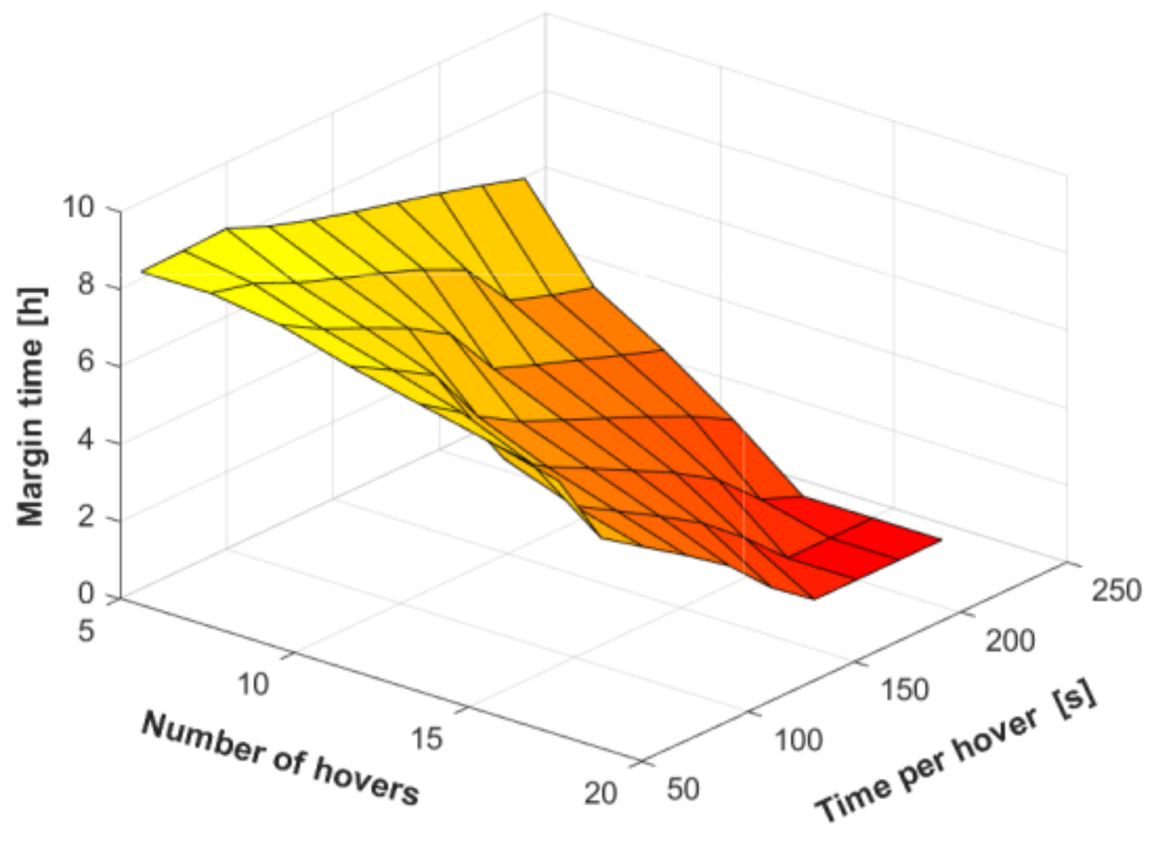
4.3.2. Effect of Mission Requirements

Figure 15 focuses on the performance of different numbers of hovers and times per hover, which was measured by margin time after completing the tasks during a mission window from 8:30 a.m. to 17:00 p.m. on 23 March. It can be observed that when the hover time increased from 60 s to 240 s under the same number of hovers, the margin time hardly changed when the number of hovers was 5five due to the fact that battery SOC can almost cover the hover missions. Because of the cloud coverage and the reduction in incoming solar energy, the margin time decreased multi-linearly. When a single time of hover was 220 s, there was no robust margin time for the SCUAV to face worse weather after the mission was completed 13 times. On the other hand, when the number of hovers increased from 5 to 17, the time per-hovering of the SCUAV decreased exponentially at the same condition. Therefore, the SOC trajectory planning of the SCUAV was achieved by matching the number of hovers and the time per hover according to the meteorological conditions in low altitude.

5. Conclusions

In this paper, a degressive SOC trajectory planning method with EMS is proposed to improve the energy usage efficiency for SCUAV driven by a multi-mode. Numerical and simulation results indicate the effectiveness and practicability of the proposed SOC trajectory planning method. The conclusions are drawn as follows:

(1)

The proposed SOC trajectory planning method with the EMS considers a solar income prediction model comprising cloud coverage, a multi-mode power model considering the direction of flow velocity and the disturbance of wind, and the full use of battery capacity. The method adopts long-term prediction and short-term dynamic error correction of the cyclic decreasing battery SOC in the multi-mode to maximize the use of the solar cell/battery and quickly complete the tasks.

(2)

An EMS of the SCUAV is proposed to control solar cell/battery output and power distribution. The implementation process is conducted according to the logical relationship ($SO{C}_{bat,i}$, $P_{sc}$ and $P_{d,i}$) in four stages driven by three modes to improve energy management efficiency.

(3)

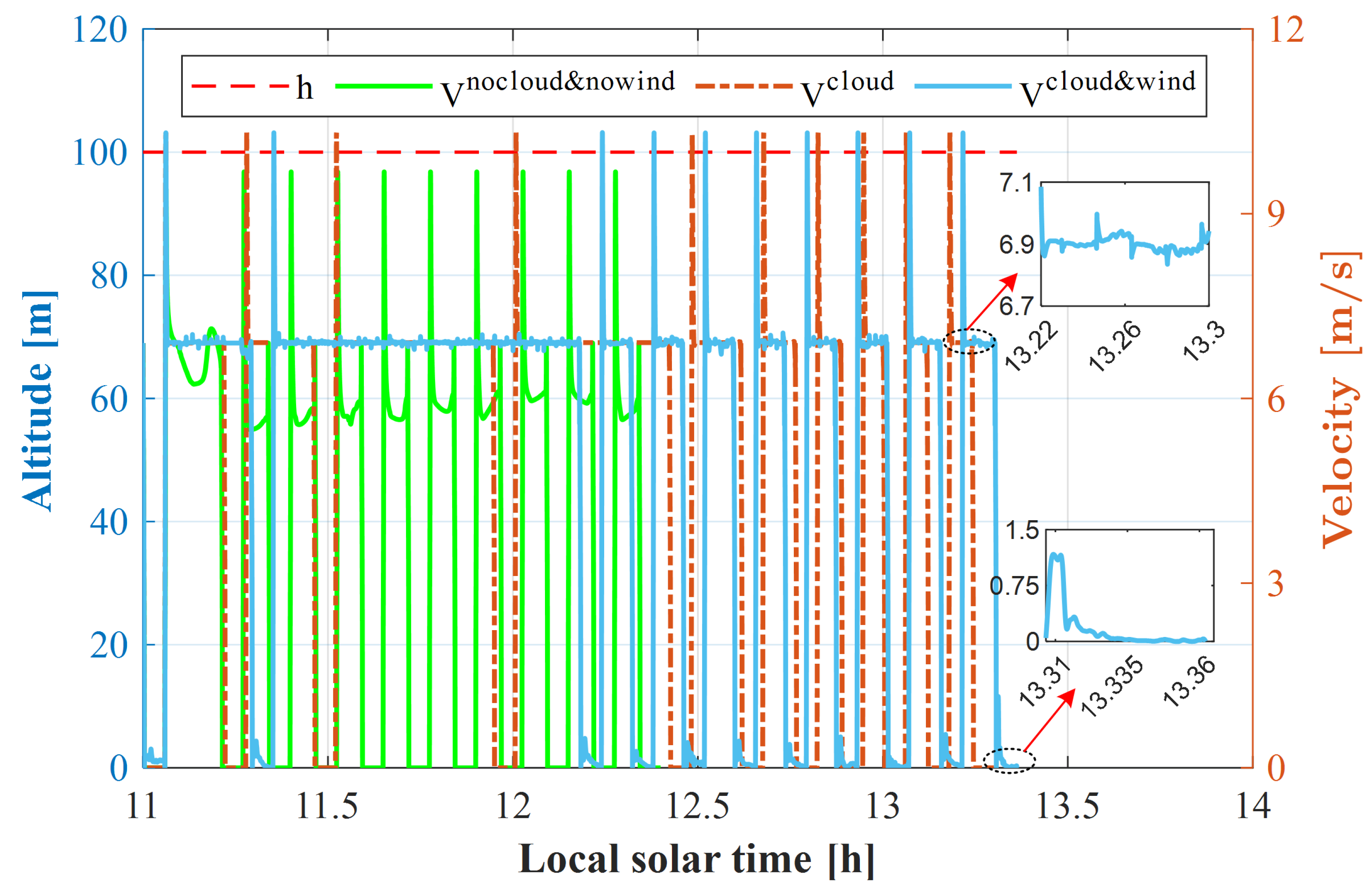
Numerical and simulation results indicate the robustness of SCUAVs under cloud coverage and wind disturbance. The endurance with cloud coverage increased by 0.56 h compared to that with clear sky with the same operation conditions. Compared with the no-wind condition, wind disturbance increased the task requirement time by 0.06 h through increasing and decreasing the propulsion power of the multi-mode for each stage.

This study shows that efficient energy trajectory planning can optimize the usage of energy and maximize mission effectiveness. It is conducive to promoting the application of solar-powered convertible aircrafts. In a follow-up study, energy trajectory planning can be coupled with energy control to improve energy management and performance.

References

1. Noth, A. Design of Solar Powered Airplanes for Continous Flight. Ph.D. Thesis, ETH Zurich, Zurich, Switzerland, 2008. [Google Scholar]
2. Zhu, X.; Guo, Z.; Hou, Z. Solar-powered airplanes: A historical perspective and future challenges. Prog. Aerosp. Sci. 2014, 71, 36–53. [Google Scholar] [CrossRef]
3. Oettershagen, P.; Melzer, A.; Mantel, T.; Rudin, K.; Stastny, T.; Wawrzacz, B.; Hinzmann, T.; Leutenegger, S.; Alexis, K.; Siegwart, R. Design of small hand-launched solar-powered UAVs: From concept study to a multi-day world endurance record flight. J. Field Robot. 2017, 34, 1352–1377. [Google Scholar] [CrossRef]
4. Danjuma, S.B.; Omar, Z.; Abdullah, M.N. Review of photovoltaic cells for solar-powered aircraft applications. Int. J. Eng. Technol. 2018, 7, 131–135. [Google Scholar]
5. Chu, Y.; Ho, C.; Lee, Y.; Li, B. Development of a solar-powered unmanned aerial vehicle for extended flight endurance. Drones 2021, 5, 44. [Google Scholar] [CrossRef]
6. Khan, N.R.; Raghorte, A.V.; Nandankar, P.V.; Waware, J.A. Solar powered UAV: A comprehensive review. In Proceedings of the AIP Conference Proceedings, Nagpur, India, 14–15 May 2022; Volume 2753. [Google Scholar]
7. D’Sa, R. Design of a Transformable Unmanned Aerial Vehicle. Ph.D. Thesis, University of Minnesota, Minneapolis, MN, USA, 2020. [Google Scholar]
8. Peciak, M.; Skarka, W.; Mateja, K.; Gude, M. Impact analysis of solar cells on vertical take-off and landing (VTOL) fixed-wing UAV. Aerospace 2023, 10, 247. [Google Scholar] [CrossRef]
9. Cao, X.; Liu, L.; Ge, J.; Yang, D. Conceptual design of long-endurance small solar-powered unmanned aerial vehicle with multiple tilts and hovers. Proc. Inst. Mech. Eng. Part G J. Aerosp. Eng. 2023, 237, 3185–3201. [Google Scholar]
10. Brandt, S.A.; Gilliam, F.T. Design analysis methodology for solar-powered aircraft. J. Aircr. 1995, 32, 703–709. [Google Scholar] [CrossRef]
11. Langelaan, J.W.; Spletzer, J.; Montella, C.; Grenestedt, J. Wind field estimation for autonomous dynamic soaring. In Proceedings of the 2012 IEEE International Conference on Robotics and Automation, Saint Paul, MN, USA, 14–18 May 2012; pp. 16–22. [Google Scholar]
12. Zhong, G.X.; Xi, H.Z.; Zheng, G.; Xia, L.J.; Qian, C.X. The influence of wind shear to the performance of high-altitude solar-powered aircraft. Proc. Inst. Mech. Eng. Part G J. Aerosp. Eng. 2014, 228, 1562–1573. [Google Scholar] [CrossRef]
13. Gao, X. Research on High-Altitude Long-Endurance Flight Based on Energy Storage by Gravitational Potential and Energy Extraction from Wind Shear; National University of Defense Technology: Changsha, China, 2014. [Google Scholar]
14. Chang, J.; Laliberté, J. Trajectory Optimization for Dynamic Soaring Remotely Piloted Aircraft with Under-Wing Solar Panels. J. Aircr. 2023, 60, 581–588. [Google Scholar] [CrossRef]
15. Klesh, A.; Kabamba, P. Energy-optimal path planning for solar-powered aircraft in level flight. In Proceedings of the AIAA Guidance, Navigation and Control Conference and Exhibit, Hilton Head, SC, USA, 20–23 August 2007; p. 6655. [Google Scholar]
16. Spangelo, S.; Gilbert, E.; Klesh, A.; Kabamba, P.; Girard, A. Periodic energy-optimal path planning for solar-powered aircraft. In Proceedings of the AIAA Guidance, Navigation, and Control Conference, Chicago, IL, USA, 10–13 August 2009; p. 6016. [Google Scholar]
17. Huang, Y.; Chen, J.; Wang, H.; Su, G. A method of 3D path planning for solar-powered UAV with fixed target and solar tracking. Aerosp. Sci. Technol. 2019, 92, 831–838. [Google Scholar] [CrossRef]
18. Hosseini, S.; Mesbahi, M. Energy-aware aerial surveillance for a long-endurance solar-powered unmanned aerial vehicles. J. Guid. Control. Dyn. 2016, 39, 1980–1993. [Google Scholar] [CrossRef]
19. Shaoqi, W.; Dongli, M.; Muqing, Y.; Liang, Z. Three-dimensional optimal path planning for high-altitude solar-powered UAV. Acta Aeronaut. Astronaut. Sin. 2019, 45, 936–943. [Google Scholar]
20. Wenjun, N.; Ying, B.; Di, W.; Xiaoping, M. Energy-optimal trajectory planning for solar-powered aircraft using soft actor-critic. Chin. J. Aeronaut. 2022, 35, 337–353. [Google Scholar]
21. Xi, Z.; Wu, D.; Ni, W.; Ma, X. Energy-optimized trajectory planning for solar-powered aircraft in a wind field using reinforcement learning. IEEE Access 2022, 10, 87715–87732. [Google Scholar] [CrossRef]
22. Boukoberine, M.N.; Zhou, Z.; Benbouzid, M. A critical review on unmanned aerial vehicles power supply and energy management: Solutions, strategies, and prospects. Appl. Energy 2019, 255, 113823. [Google Scholar] [CrossRef]
23. Lei, T.; Min, Z.; Gao, Q.; Song, L.; Zhang, X.; Zhang, X. The architecture optimization and energy management technology of aircraft power systems: A review and future trends. Energies 2022, 15, 4109. [Google Scholar] [CrossRef]
24. Gao, X.Z.; Hou, Z.X.; Guo, Z.; Liu, J.X.; Chen, X.Q. Energy management strategy for solar-powered high-altitude long-endurance aircraft. Energy Convers. Manag. 2013, 70, 20–30. [Google Scholar] [CrossRef]
25. Sun, M.; Shan, C.; Sun, K.-w.; Jia, Y.-h. Energy Management Strategy for High-Altitude Solar Aircraft Based on Multiple Flight Phases. Math. Probl. Eng. 2020, 2020, 6655031. [Google Scholar] [CrossRef]
26. Wang, F.; Sun, X.; He, X.; Zhuo, F.; Yi, H. Research on Energy Optimal Control Strategy of DC PV-Energy Storage System for Unmanned Aerial Vehicle. IEEE J. Emerg. Sel. Top. Power Electron. 2020, 9, 2643–2651. [Google Scholar] [CrossRef]
27. Qi, N.; Dai, K.; Yi, F.; Wang, X.; You, Z.; Zhao, J. An adaptive energy management strategy to extend battery lifetime of solar powered wireless sensor nodes. IEEE Access 2019, 7, 88289–88300. [Google Scholar] [CrossRef]
28. Wang, H.; Li, P.; Xiao, H.; Zhou, X.; Lei, R. Intelligent energy management for solar-powered unmanned aerial vehicle using multi-objective genetic algorithm. Energy Convers. Manag. 2023, 280, 116805. [Google Scholar] [CrossRef]
29. Ahmad, T.; Zhang, H.; Yan, B. A review on renewable energy and electricity requirement forecasting models for smart grid and buildings. Sustain. Cities Soc. 2020, 55, 102052. [Google Scholar] [CrossRef]
30. Aslam, S.; Herodotou, H.; Mohsin, S.M.; Javaid, N.; Ashraf, N.; Aslam, S. A survey on deep learning methods for power load and renewable energy forecasting in smart microgrids. Renew. Sustain. Energy Rev. 2021, 144, 110992. [Google Scholar] [CrossRef]
31. Blaga, R.; Sabadus, A.; Stefu, N.; Dughir, C.; Paulescu, M.; Badescu, V. A current perspective on the accuracy of incoming solar energy forecasting. Prog. Energy Combust. Sci. 2019, 70, 119–144. [Google Scholar] [CrossRef]
32. Rahimi, N.; Park, S.; Choi, W.; Oh, B.; Kim, S.; Cho, Y.h.; Ahn, S.; Chong, C.; Kim, D.; Jin, C.; et al. A Comprehensive Review on Ensemble Solar Power Forecasting Algorithms. J. Electr. Eng. Technol. 2023, 18, 719–733. [Google Scholar] [CrossRef]
33. Krishnan, N.; Kumar, K.R.; Inda, C.S. How solar radiation forecasting impacts the utilization of solar energy: A critical review. J. Clean. Prod. 2023, 388, 135860. [Google Scholar] [CrossRef]
34. Cheng, L.; Zang, H.; Trivedi, A.; Srinivasan, D.; Ding, T.; Wei, Z.; Sun, G. Prediction of Non-Stationary Multi-Head Cloud Motion Vectors for Intra-Hourly Satellite-Derived Solar Power Forecasting. IEEE Trans. Power Syst. 2023. [Google Scholar] [CrossRef]
35. Yang, D.; Yang, G.; Liu, B. Combining quantiles of calibrated solar forecasts from ensemble numerical weather prediction. Renew. Energy 2023, 215, 118993. [Google Scholar] [CrossRef]
36. Abou Houran, M.; Bukhari, S.M.S.; Zafar, M.H.; Mansoor, M.; Chen, W. COA-CNN-LSTM: Coati optimization algorithm-based hybrid deep learning model for PV/wind power forecasting in smart grid applications. Appl. Energy 2023, 349, 121638. [Google Scholar] [CrossRef]
37. Huang, X.; Liu, J.; Xu, S.; Li, C.; Li, Q.; Tai, Y. A 3D ConvLSTM-CNN network based on multi-channel color extraction for ultra-short-term solar irradiance forecasting. Energy 2023, 272, 127140. [Google Scholar] [CrossRef]
38. Ajith, M.; Martínez-Ramón, M. Deep learning algorithms for very short term solar irradiance forecasting: A survey. Renew. Sustain. Energy Rev. 2023, 182, 113362. [Google Scholar] [CrossRef]
39. Perne, M.; Kocijan, J.; Božnar, M.; Grašič, B.; Mlakar, P. Hybrid Forecasting of Wind for Air Pollution Dispersion over Complex Terrain. J. Environ. Inform. 2023, 41, 88–103. [Google Scholar] [CrossRef]
40. Yang, B.; Zhong, L.; Wang, J.; Shu, H.; Zhang, X.; Yu, T.; Sun, L. State-of-the-art one-stop handbook on wind forecasting technologies: An overview of classifications, methodologies, and analysis. J. Clean. Prod. 2021, 283, 124628. [Google Scholar] [CrossRef]
41. Liu, M.D.; Ding, L.; Bai, Y.L. Application of hybrid model based on empirical mode decomposition, novel recurrent neural networks and the ARIMA to wind speed prediction. Energy Convers. Manag. 2021, 233, 113917. [Google Scholar] [CrossRef]
42. Ding, L.; Bai, Y.L.; Fan, M.H.; Yu, Q.H.; Zhu, Y.J.; Chen, X.Y. Serial-parallel dynamic echo state network: A hybrid dynamic model based on a chaotic coyote optimization algorithm for wind speed prediction. Expert Syst. Appl. 2023, 212, 118789. [Google Scholar] [CrossRef]
43. Khan, W.; Nahon, M. A propeller model for general forward flight conditions. Int. J. Intell. Unmanned Syst. 2015, 3, 72–92. [Google Scholar] [CrossRef]
44. Hu, S.; Ni, W.; Wang, X.; Jamalipour, A. Disguised Tailing and Video Surveillance with Solar-Powered Fixed-Wing Unmanned Aerial Vehicle. IEEE Trans. Veh. Technol. 2022, 71, 5507–5518. [Google Scholar] [CrossRef]
45. Oettershagen, P. High-fidelity solar power income modeling for solar-electric uavs: Development and flight test based verification. arXiv 2017, arXiv:1703.07385. [Google Scholar]
46. Ju, C.; Wang, P.; Goel, L.; Xu, Y. A Two-layer Energy Management System for Microgrids with Hybrid Energy Storage considering Degradation Costs. IEEE Trans. Smart Grid 2017, 9, 6047–6057. [Google Scholar] [CrossRef]
47. Mallat, S.G. A theory for multiresolution signal decomposition: The wavelet representation. IEEE Trans. Pattern Anal. Mach. Intell. 1989, 11, 674–693. [Google Scholar] [CrossRef]
48. APC. 2003. Available online: https://www.apcprop.com/technical-information/performance-data/ (accessed on 17 January 2024).
49. Brandt, J.; Selig, M. Propeller performance data at low reynolds numbers. In Proceedings of the 49th AIAA Aerospace Sciences Meeting including the New Horizons Forum and Aerospace Exposition, Orlando, FL, USA, 4–7 January 2011; p. 1255. [Google Scholar]
50. Andreas, A.; Wilcox, S. Solar Technology Acceleration Center (SolarTAC). 2011. Available online: https://midcdmz.nrel.gov/apps/sitehome.pl?site=STAC (accessed on 11 February 2011).
51. Yu, Z. Research on Tilt-Rotor UAV Transition Strategy. Master’s Thesis, Beijing Institute of Technology, Beijing, China, 2020. [Google Scholar]
Figure 1. Specific mission profile of SCUAV.
Drones 08 00080 g001
Figure 2. Diagram of hybrid solar cell/battery power topology.
Drones 08 00080 g002
Figure 3. Propeller angle of attack on the aerodynamic forces.
Drones 08 00080 g003
Figure 4. Framework of degressive SOC trajectory planning.
Drones 08 00080 g004
Figure 5. Diagram of hybrid energy showing input power, output power and battery energy.
Drones 08 00080 g005
Figure 6. Hybrid WT-LSTM-ARIMA prediction model.
Drones 08 00080 g006
Figure 7. Multi-mode SOC trajectory optimization of the SCUAV.
Drones 08 00080 g007
Figure 8. Comparison diagram of the propeller model.
Drones 08 00080 g008
Figure 9. Sample data of solar irradiance and wind. (a) Solar irradiance training; (b) solar irradiance testing; (c) wind training; (d) wind testing.
Drones 08 00080 g009
Figure 10. Comparison diagram of SOC trajectory planning. (a) With or without cloud; (b) with or without wind.
Drones 08 00080 g010
Figure 11. Comparison diagram of propeller speed. (a) With or without cloud; (b) with or without wind.
Drones 08 00080 g011
Figure 12. Comparison diagram of the tilt angle.
Drones 08 00080 g012
Figure 13. Comparison diagram of velocity.
Drones 08 00080 g013
Figure 14. Comparison of trajectory planning strategies for fixed value and degression of SOC.
Drones 08 00080 g014
Figure 15. Performance of the SCUAV with different hovering missions.
Drones 08 00080 g015