

SSMA-YOLO: A Lightweight YOLO Model with Enhanced Feature Extraction and Fusion Capabilities for Drone-Aerial Ship Image Detection


Abstract
1. Introduction
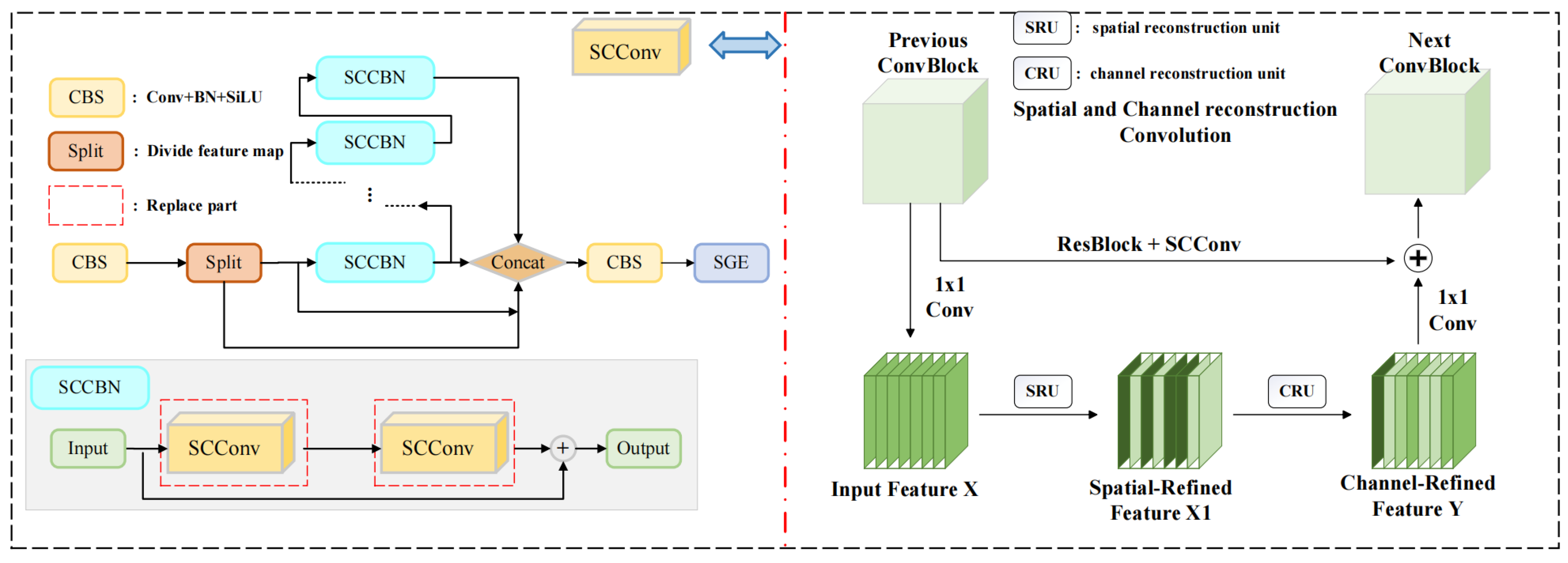
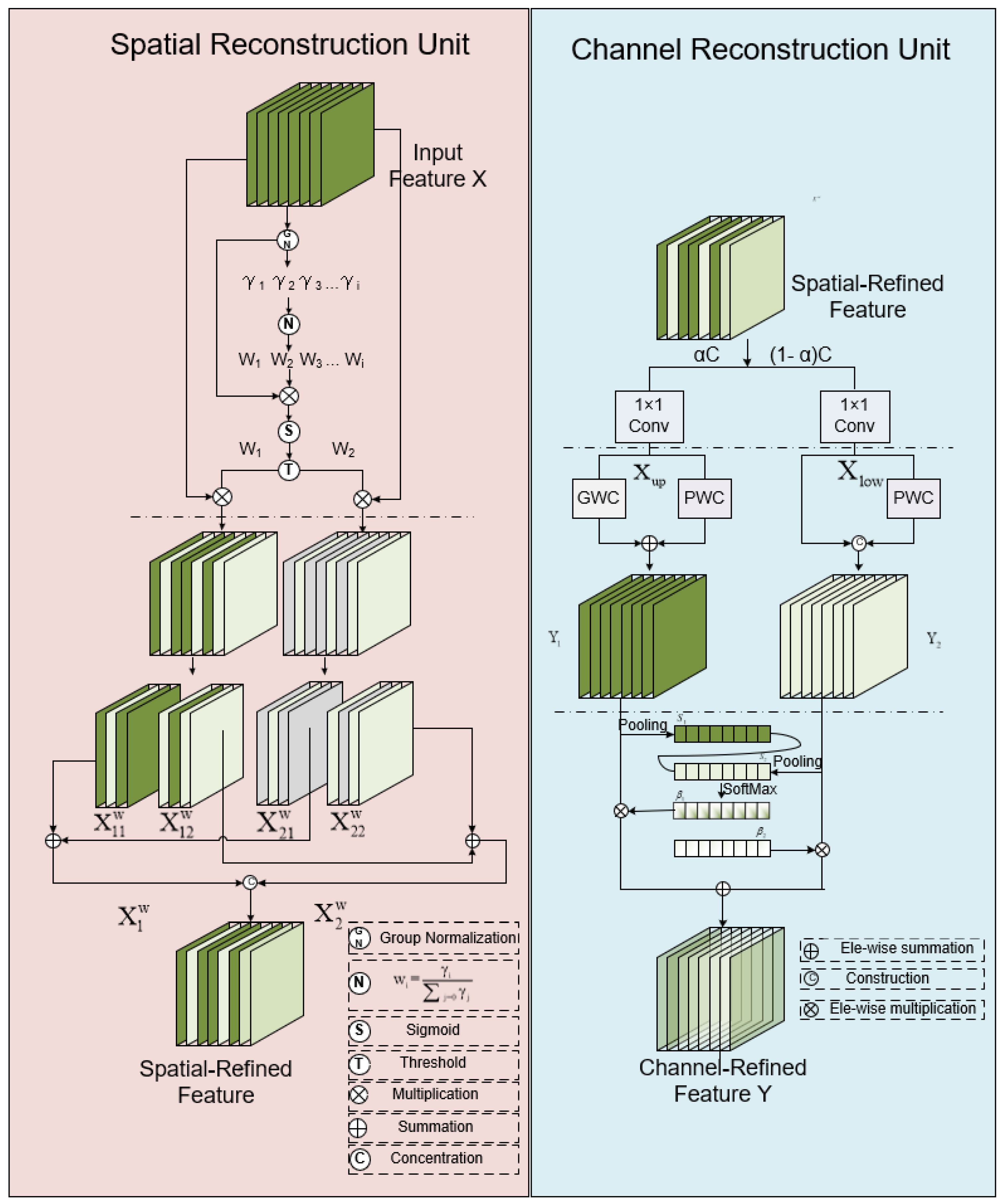
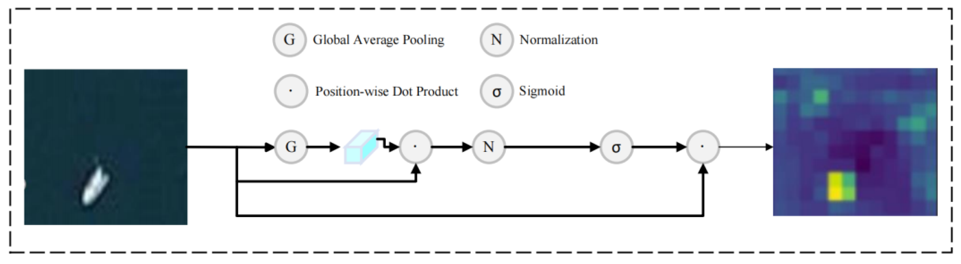
- We employ GhostConv to replace traditional convolutions in the backbone and neck layers and introduce a plug-and-play SSC2f module. This module utilizes a newly designed SCCBN to replace the traditional Bottleneck. Through the separation and reconstruction of features, it reduces spatial and channel redundancy in convolutional neural networks. Additionally, the module incorporates the SGE attention mechanism, which adjusts the importance of each factor based on every spatial location within each semantic group, thereby enhancing precision.
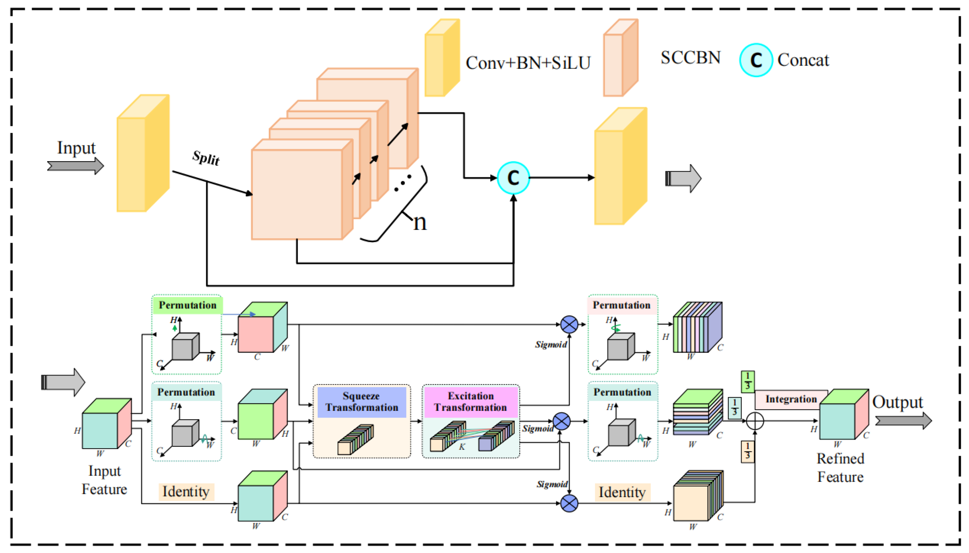
- To enhance the model’s ability to efficiently process key information against complex backgrounds, a lightweight module named MC2f is proposed. This module employs the MCA attention mechanism to effectively capture spatial and channel features across three dimensions, thereby improving the model’s capability to extract information from complex backgrounds.
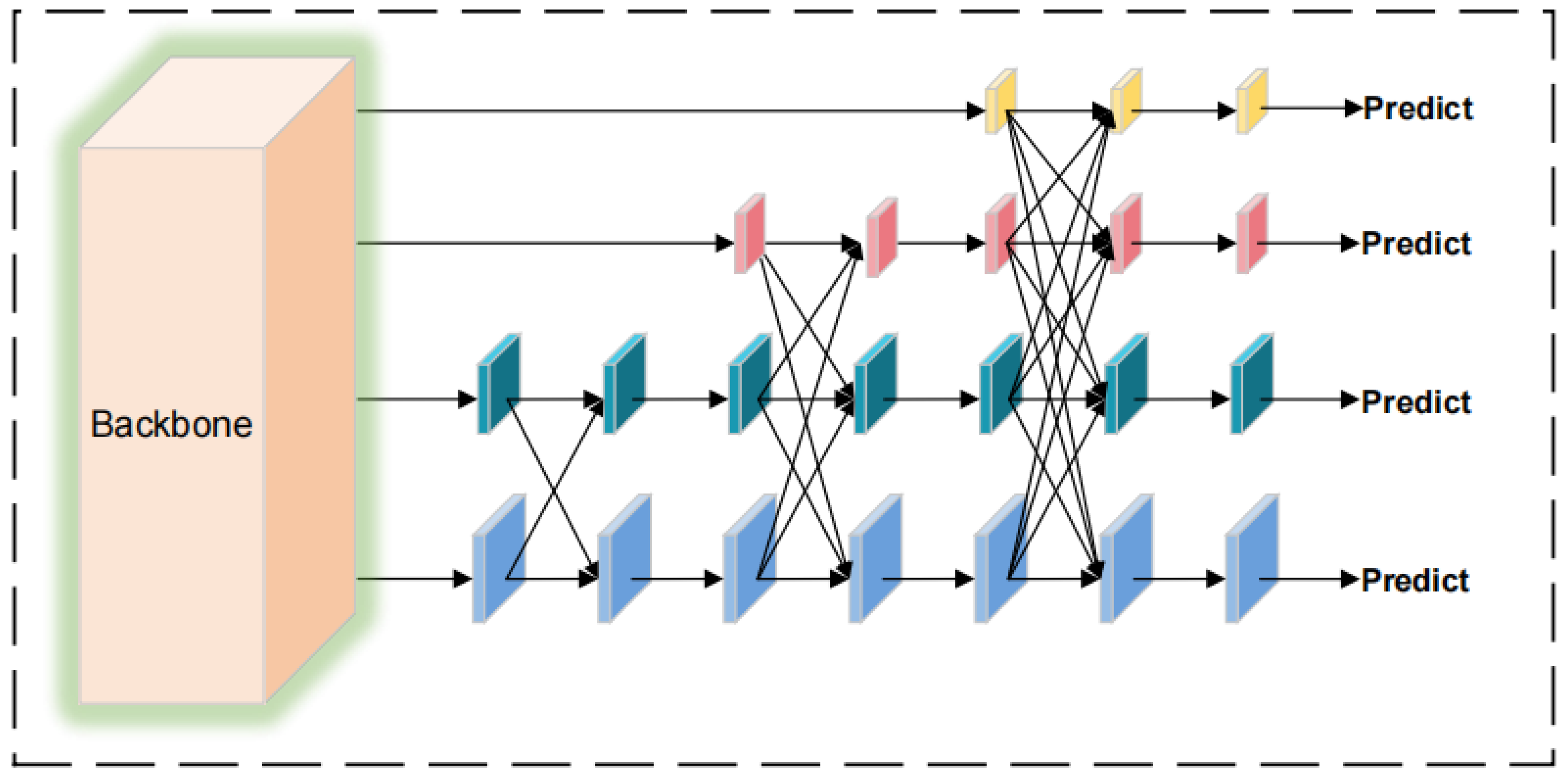
- To address the poor feature fusion capability of the YOLOv8n model’s FPN + APN module for multi-scale targets, this paper achieves optimization using the AFPN structure, progressively fusing features and effectively suppressing information contradictions between different levels. This optimization improves the selection and fusion process of features, enhancing the model’s focus on key features. The result is improved target recognition accuracy when facing multi-target scale problems.
2. Materials and Methods
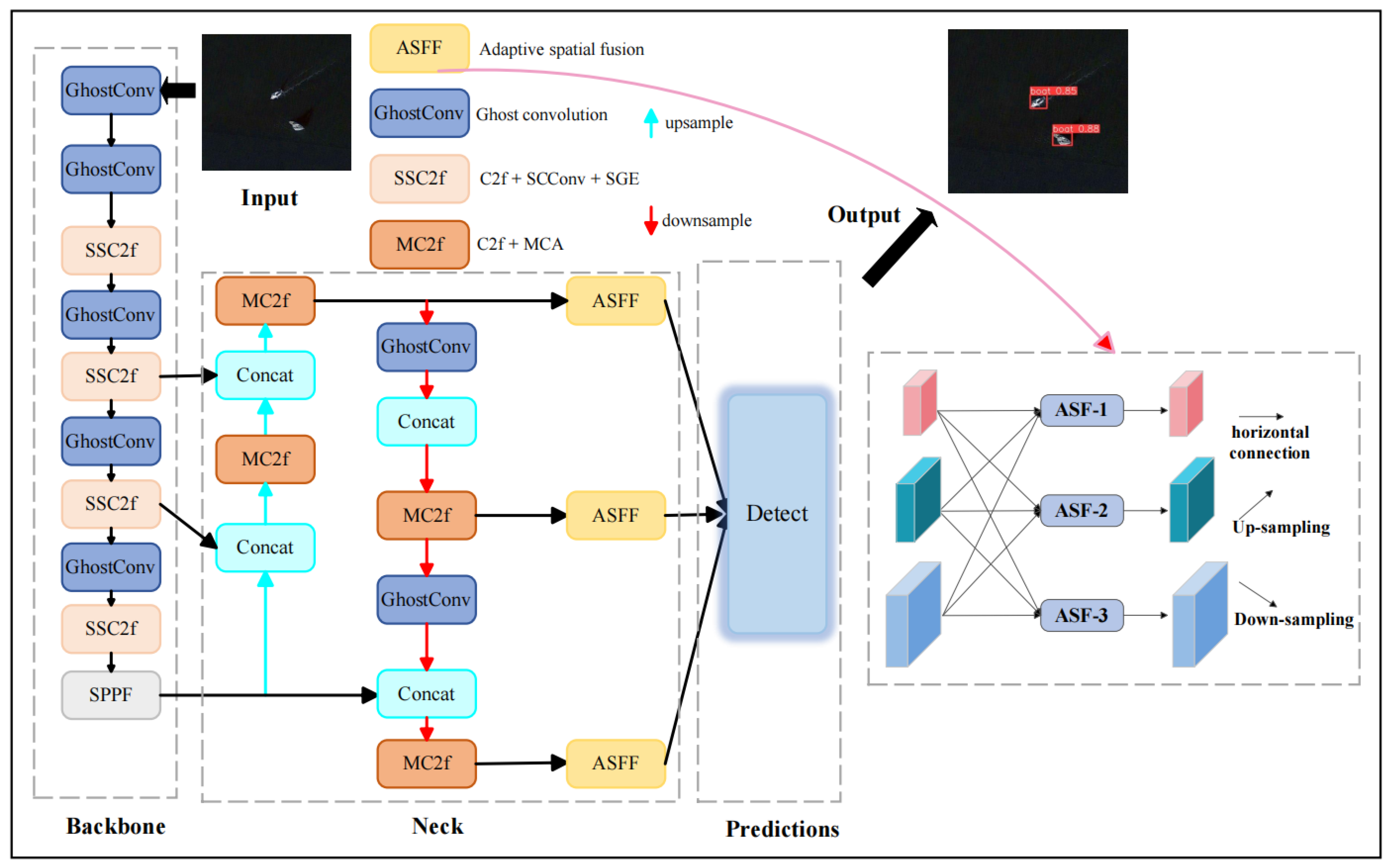
2.1. SSMA-YOLO
2.2. Model Lightweight Optimization
2.3. Optimization of Complex-Scene Recognition
2.4. Optimization of Multi-Scale Target Recognition Accuracy
3. Results
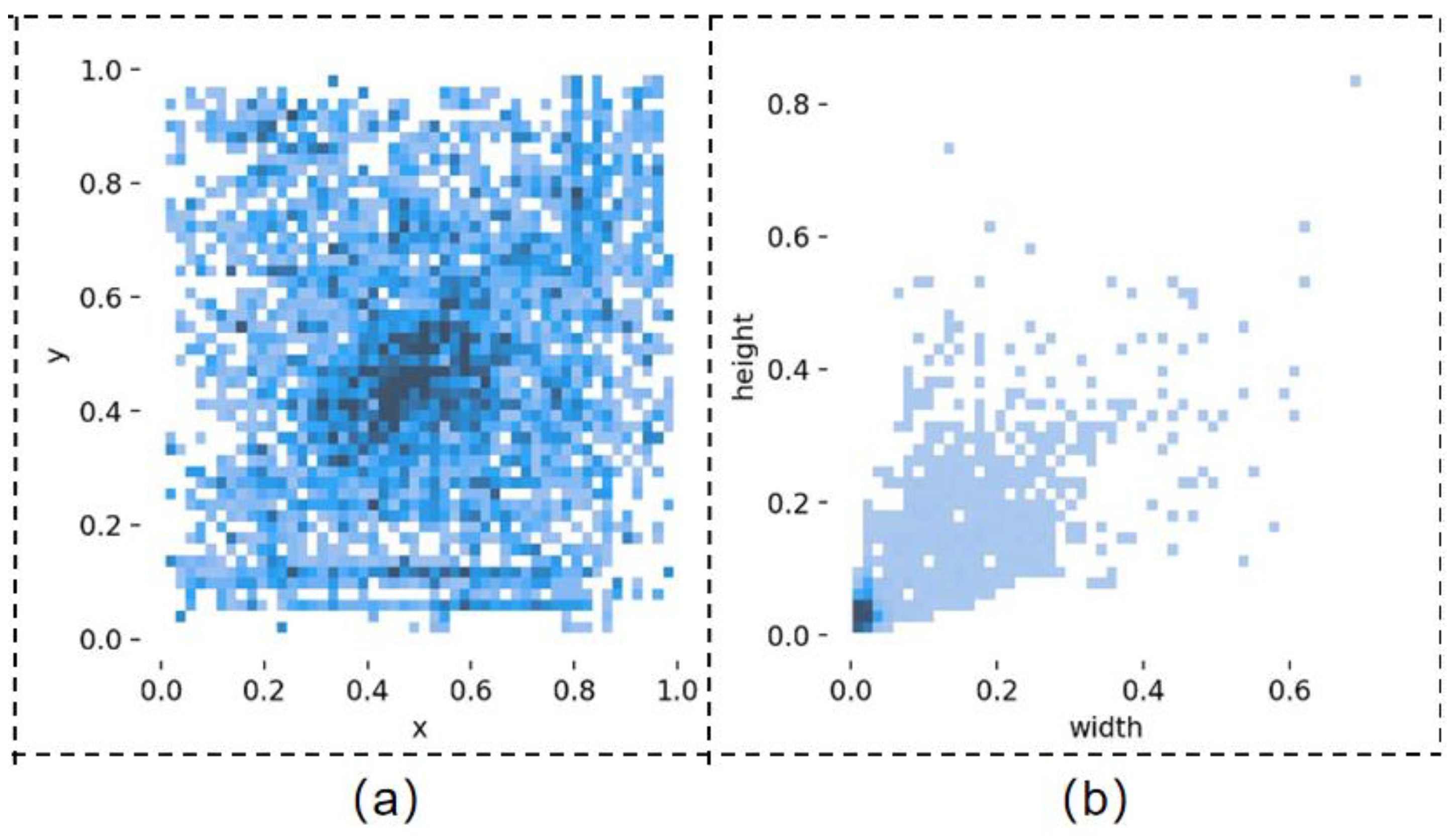
3.1. Dataset
3.2. Environment and Evaluation
- (1)
- TP, FP, TN, FN
- (2)
- Recall and Precision
- (3)
- F1
- (4)
- AP and mAP
- (5)
- Weights, parameters, and FLOPs
3.3. Experimental Result
3.3.1. Comparative Experiment after Model Optimization
3.3.2. Ablation Experiment
3.3.3. Comparison with Other Models
3.3.4. Generalization Test
4. Discussion
5. Conclusions
Author Contributions
Funding
Data Availability Statement
Conflicts of Interest
References
- Arivazhagan, S.; Lilly Jebarani, W.S.; Newlin Shebiah, R.; Ligi, S.V.; Hareesh Kumar, P.V.; Anilkumar, K. Significance Based Ship Detection from SAR Imagery. In Proceedings of the 2019 1st International Conference on Innovations in Information and Communication Technology (ICIICT), Chennai, India, 25–26 April 2019; pp. 1–5. [Google Scholar]
- Dominguez-Péry, C.; Tassabehji, R.; Corset, F.; Chreim, Z. A Holistic View of Maritime Navigation Accidents and Risk Indicators: Examining IMO Reports from 2011 to 2021. J. Shipp. Trade 2023, 8, 11. [Google Scholar] [CrossRef]
- Goerlandt, F.; Goite, H.; Banda, O.A.V.; Höglund, A.; Ahonen-Rainio, P.; Lensu, M. An Analysis of Wintertime Navigational Accidents in the Northern Baltic Sea. Saf. Sci. 2017, 92, 66–84. [Google Scholar] [CrossRef]
- Goerlandt, F.; Montewka, J. Maritime Transportation Risk Analysis: Review and Analysis in Light of Some Foundational Issues. Reliab. Eng. Syst. Saf. 2015, 138, 115–134. [Google Scholar] [CrossRef]
- Teixeira, E.; Araujo, B.; Costa, V.; Mafra, S.; Figueiredo, F. Literature Review on Ship Localization, Classification, and Detection Methods Based on Optical Sensors and Neural Networks. Sensors 2022, 22, 6879. [Google Scholar] [CrossRef] [PubMed]
- Crow’s Nest. Wikipedia 2023. Available online: https://en.wikipedia.org/w/index.php?title=Crow%27s_nest&oldid=1186905465 (accessed on 6 April 2024).
- Lu, Z.; Wang, P.; Li, Y.; Ding, B. A New Deep Neural Network Based on SwinT-FRM-ShipNet for SAR Ship Detection in Complex Near-Shore and Offshore Environments. Remote Sens. 2023, 15, 5780. [Google Scholar] [CrossRef]
- Tian, Y.; Wang, X.; Zhu, S.; Xu, F.; Liu, J. LMSD-Net: A Lightweight and High-Performance Ship Detection Network for Optical Remote Sensing Images. Remote Sens. 2023, 15, 4358. [Google Scholar] [CrossRef]
- Yasir, M.; Niang, A.J.; Hossain, M.S.; Islam, Q.U.; Yang, Q.; Yin, Y. Ranking Ship Detection Methods Using SAR Images Based on Machine Learning and Artificial Intelligence. J. Mar. Sci. Eng. 2023, 11, 1916. [Google Scholar] [CrossRef]
- Cao, X.; Gao, S.; Chen, L.; Wang, Y. Ship Recognition Method Combined with Image Segmentation and Deep Learning Feature Extraction in Video Surveillance. Multimed. Tools Appl. 2020, 79, 9177–9192. [Google Scholar] [CrossRef]
- Xing, X.; Ji, K.; Zou, H.; Sun, J. Feature Selection and Weighted SVM Classifier-Based Ship Detection in PolSAR Imagery. Int. J. Remote Sens. 2013, 34, 7925–7944. [Google Scholar] [CrossRef]
- He, J.; Hao, Y.; Wang, X. An Interpretable Aid Decision-Making Model for Flag State Control Ship Detention Based on SMOTE and XGBoost. J. Mar. Sci. Eng. 2021, 9, 156. [Google Scholar] [CrossRef]
- Yan, Z.; Song, X.; Yang, L.; Wang, Y. Ship Classification in Synthetic Aperture Radar Images Based on Multiple Classifiers Ensemble Learning and Automatic Identification System Data Transfer Learning. Remote Sens. 2022, 14, 5288. [Google Scholar] [CrossRef]
- Zhao, Z.-Q.; Zheng, P.; Xu, S.; Wu, X. Object Detection with Deep Learning: A Review. IEEE Trans. Neural Netw. Learn. Syst. 2019, 30, 3212–3232. [Google Scholar] [CrossRef]
- Chen, C.; Zheng, Z.; Xu, T.; Guo, S.; Feng, S.; Yao, W.; Lan, Y. YOLO-Based UAV Technology: A Review of the Research and Its Applications. Drones 2023, 7, 190. [Google Scholar] [CrossRef]
- Liu, J.; Guan, R.; Li, Z.; Zhang, J.; Hu, Y.; Wang, X. Adaptive Multi-Feature Fusion Graph Convolutional Network for Hyperspectral Image Classification. Remote Sens. 2023, 15, 5483. [Google Scholar] [CrossRef]
- Guan, R.; Li, Z.; Li, T.; Li, X.; Yang, J.; Chen, W. Classification of Heterogeneous Mining Areas Based on ResCapsNet and Gaofen-5 Imagery. Remote Sens. 2022, 14, 3216. [Google Scholar] [CrossRef]
- Guan, R.; Li, Z.; Tu, W.; Wang, J.; Liu, Y.; Li, X.; Tang, C.; Feng, R. Contrastive Multi-View Subspace Clustering of Hyperspectral Images Based on Graph Convolutional Networks. IEEE Trans. Geosci. Remote Sens. 2024, 62, 5510514. [Google Scholar] [CrossRef]
- Guan, R.; Li, Z.; Li, X.; Tang, C. Pixel-Superpixel Contrastive Learning and Pseudo-Label Correction for Hyperspectral Image Clustering. In Proceedings of the ICASSP 2024-2024 IEEE International Conference on Acoustics, Speech and Signal Processing (ICASSP), Seoul, Republic of Korea, 14–19 April 2024; IEEE: New York, NY, USA, 2024; pp. 6795–6799. [Google Scholar]
- Han, X.; Zhao, L.; Ning, Y.; Hu, J. ShipYolo: An Enhanced Model for Ship Detection. J. Adv. Transp. 2021, 2021, 1060182. [Google Scholar] [CrossRef]
- Kouvaras, L.; Petropoulos, G.P. A Novel Technique Based on Machine Learning for Detecting and Segmenting Trees in Very High Resolution Digital Images from Unmanned Aerial Vehicles. Drones 2024, 8, 43. [Google Scholar] [CrossRef]
- Zhang, Z. Drone-YOLO: An Efficient Neural Network Method for Target Detection in Drone Images. Drones 2023, 7, 526. [Google Scholar] [CrossRef]
- Girshick, R.; Donahue, J.; Darrell, T.; Malik, J. Region-Based Convolutional Networks for Accurate Object Detection and Segmentation. IEEE Trans. Pattern Anal. Mach. Intell. 2015, 38, 142–158. [Google Scholar] [CrossRef]
- Li, Y.; Zhang, S.; Wang, W.-Q. A Lightweight Faster R-CNN for Ship Detection in SAR Images. IEEE Geosci. Remote Sens. Lett. 2020, 19, 4006105. [Google Scholar] [CrossRef]
- Jiao, J.; Zhang, Y.; Sun, H.; Yang, X.; Gao, X.; Hong, W.; Fu, K.; Sun, X. A Densely Connected End-to-End Neural Network for Multiscale and Multiscene SAR Ship Detection. IEEE Access 2018, 6, 20881–20892. [Google Scholar] [CrossRef]
- Zhou, Y.; Jiang, W.; Jiang, X.; Chen, L.; Liu, X. CamoNet: A Target Camouflage Network for Remote Sensing Images Based on Adversarial Attack. Remote Sens. 2023, 15, 5131. [Google Scholar] [CrossRef]
- Yu, M.; Han, S.; Wang, T.; Wang, H. An Approach to Accurate Ship Image Recognition in a Complex Maritime Transportation Environment. J. Mar. Sci. Eng. 2022, 10, 1903. [Google Scholar] [CrossRef]
- Yu, L.; Wu, H.; Zhong, Z.; Zheng, L.; Deng, Q.; Hu, H. TWC-Net: A SAR Ship Detection Using Two-Way Convolution and Multiscale Feature Mapping. Remote Sens. 2021, 13, 2558. [Google Scholar] [CrossRef]
- Redmon, J.; Divvala, S.; Girshick, R.; Farhadi, A. You Only Look Once: Unified, Real-Time Object Detection. In Proceedings of the IEEE Conference on Computer Vision and Pattern Recognition, Las Vegas, NV, USA, 27–30 June 2016. [Google Scholar]
- Tang, G.; Liu, S.; Fujino, I.; Claramunt, C.; Wang, Y.; Men, S. H-YOLO: A Single-Shot Ship Detection Approach Based on Region of Interest Preselected Network. Remote Sens. 2020, 12, 4192. [Google Scholar] [CrossRef]
- Jiang, J.; Fu, X.; Qin, R.; Wang, X.; Ma, Z. High-Speed Lightweight Ship Detection Algorithm Based on YOLO-v4 for Three-Channels RGB SAR Image. Remote Sens. 2021, 13, 1909. [Google Scholar] [CrossRef]
- Xu, X.; Zhang, X.; Zhang, T. Lite-Yolov5: A Lightweight Deep Learning Detector for on-Board Ship Detection in Large-Scene Sentinel-1 Sar Images. Remote Sens. 2022, 14, 1018. [Google Scholar] [CrossRef]
- Chen, Z.; Liu, C.; Filaretov, V.F.; Yukhimets, D.A. Multi-Scale Ship Detection Algorithm Based on YOLOv7 for Complex Scene SAR Images. Remote Sens. 2023, 15, 2071. [Google Scholar] [CrossRef]
- Zhao, X.; Song, Y. Improved Ship Detection with YOLOv8 Enhanced with MobileViT and GSConv. Electronics 2023, 12, 4666. [Google Scholar] [CrossRef]
- Liang, H.; Lee, S.-C.; Seo, S. UAV-Based Low Altitude Remote Sensing for Concrete Bridge Multi-Category Damage Automatic Detection System. Drones 2023, 7, 386. [Google Scholar] [CrossRef]
- Li, X.; Zhu, R.; Yu, X.; Wang, X. High-Performance Detection-Based Tracker for Multiple Object Tracking in UAVs. Drones 2023, 7, 681. [Google Scholar] [CrossRef]
- GitHub-Ultralytics/Ultralytics: NEW-YOLOv8 🚀 in PyTorch > ONNX > OpenVINO > CoreML > TFLite. Available online: https://github.com/ultralytics/ultralytics (accessed on 16 January 2024).
- Ge, Z.; Liu, S.; Wang, F.; Li, Z.; Sun, J. YOLOX: Exceeding YOLO Series in 2021. arXiv 2021, arXiv:2107.08430. [Google Scholar]
- Hu, J.; Shen, L.; Sun, G. Squeeze-and-Excitation Networks. In Proceedings of the IEEE Conference on Computer Vision and Pattern Recognition, Salt Lake City, UT, USA, 18–23 June 2018; pp. 7132–7141. [Google Scholar]
- Ships/Vessels in Aerial Images. Available online: https://www.kaggle.com/datasets/siddharthkumarsah/ships-in-aerial-images (accessed on 16 January 2024).
- Ren, S.; He, K.; Girshick, R.; Sun, J. Faster R-Cnn: Towards Real-Time Object Detection with Region Proposal Networks. IEEE Trans. Pattern Anal. Mach. Intell. 2016, 39, 1137–1149. [Google Scholar] [CrossRef] [PubMed]
- Liu, W.; Anguelov, D.; Erhan, D.; Szegedy, C.; Reed, S.; Fu, C.-Y.; Berg, A.C. SSD: Single Shot MultiBox Detector. In Computer Vision–ECCV 2016; Leibe, B., Matas, J., Sebe, N., Welling, M., Eds.; Lecture Notes in Computer Science; Springer International Publishing: Cham, Switzerland, 2016; Volume 9905, pp. 21–37. ISBN 978-3-319-46447-3. [Google Scholar]
- Redmon, J.; Farhadi, A. Yolov3: An Incremental Improvement. arXiv 2018, arXiv:1804.02767. [Google Scholar]
- Wu, W.; Liu, H.; Li, L.; Long, Y.; Wang, X.; Wang, Z.; Li, J.; Chang, Y. Application of Local Fully Convolutional Neural Network Combined with YOLO v5 Algorithm in Small Target Detection of Remote Sensing Image. PLoS ONE 2021, 16, e0259283. [Google Scholar] [CrossRef]
- Wang, C.-Y.; Bochkovskiy, A.; Liao, H.-Y.M. YOLOv7: Trainable Bag-of-Freebies Sets New State-of-the-Art for Real-Time Object Detectors. In Proceedings of the IEEE/CVF Conference on Computer Vision and Pattern Recognition, Vancouver, BC, Canada, 17–24 June 2023; pp. 7464–7475. [Google Scholar]
- Zhang, T.; Zhang, X.; Li, J.; Xu, X.; Wang, B.; Zhan, X.; Xu, Y.; Ke, X.; Zeng, T.; Su, H.; et al. SAR Ship Detection Dataset (SSDD): Official Release and Comprehensive Data Analysis. Remote Sens. 2021, 13, 3690. [Google Scholar] [CrossRef]
- Papers with Code-HRSC2016 Dataset. Available online: https://paperswithcode.com/dataset/hrsc2016 (accessed on 19 January 2024).


| Model | Precision (%) | Recall (%) | F1 (%) | mAP (%) | Parameters (M) |
|---|---|---|---|---|---|
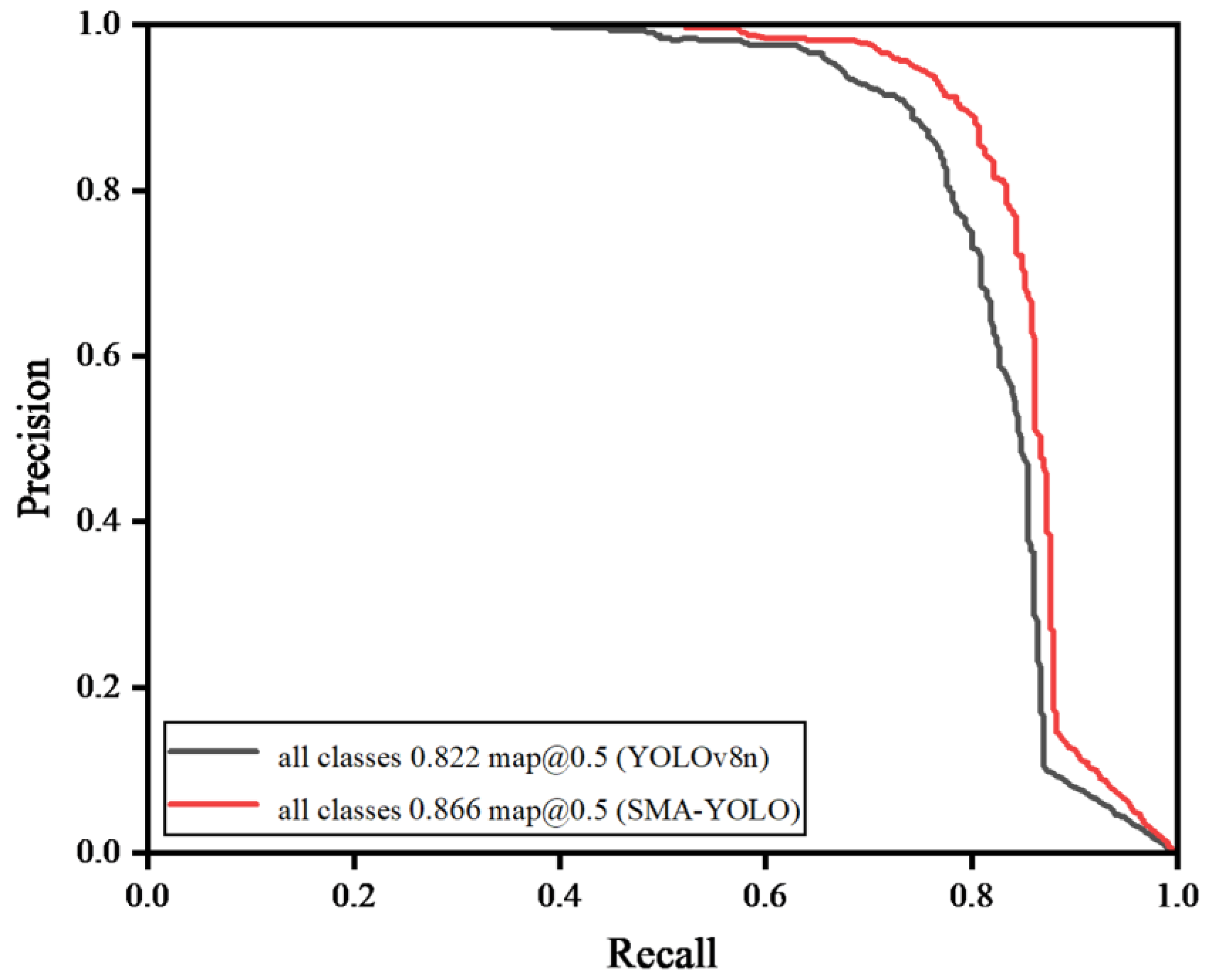
| YOLOv8n | 88.4 | 74.6 | 80.9 | 82.2 | 3.0 |
| SSMA-YOLO | 91.6 | 79.4 | 85.1 | 86.6 | 2.3 |
| Model | mAP (%) | Recall (%) | F1(%) | Precision (%) | FLOPs (G) |
|---|---|---|---|---|---|
| YOLOv8n | 82.2 | 74.6 | 80.9 | 88.4 | 8.1 |
| YOLOv8n + S 1 | 81.3 | 73.9 | 80.0 | 87.2 | 6.8 |
| YOLOv8n + S + M 2 | 84.5 | 78.2 | 83.4 | 89.3 | 6.8 |
| YOLOv8n + S + M + A 3 | 86.6 | 79.4 | 85.1 | 91.6 | 6.8 |
| Model | Precision (%) | Recall (%) | F1 (%) | mAP (%) |
|---|---|---|---|---|
| Faster-RCNN | 80.8 | 70.1 | 75.1 | 77.4 |
| SSD | 82.9 | 72.6 | 74.4 | 78.2 |
| YOLOv3 | 83.7 | 73.4 | 78.2 | 79.6 |
| YOLOv5 | 85.4 | 73.7 | 79.1 | 80.7 |
| YOLOv7 | 87.6 | 74.2 | 80.3 | 81.8 |
| SSMA-YOLO | 91.6 | 79.4 | 85.1 | 86.6 |
| Dataset | Model | Precision (%) | Recall (%) | F1 (%) | mAP (%) |
|---|---|---|---|---|---|
| HRSC-2016 | Faster-RCNN | 84.3 | 81.4 | 82.8 | 84.5 |
| SSD | 86.1 | 83.2 | 84.6 | 87.8 | |
| YOLOv3 | 87.3 | 84.4 | 85.8 | 89.1 | |
| YOLOv5 | 88.4 | 85.7 | 87.0 | 90.7 | |
| YOLOv7 | 90.6 | 86.2 | 88.3 | 91.8 | |
| YOLOv8n | 93.1 | 90.3 | 91.7 | 95.9 | |
| SSMA-YOLO | 95.7 | 95.4 | 95.5 | 97.3 | |
| SSDD | Faster-RCNN | 83.9 | 80.2 | 82.0 | 79.9 |
| SSD | 84.5 | 82.1 | 83.3 | 80.6 | |
| YOLOv3 | 85.2 | 83.4 | 84.3 | 82.2 | |
| YOLOv5 | 86.8 | 84.2 | 85.5 | 83.4 | |
| YOLOv7 | 88.6 | 85.6 | 87.1 | 84.8 | |
| YOLOv8n | 91.3 | 87.3 | 89.3 | 86.9 | |
| SSMA-YOLO | 93.2 | 89.2 | 91.2 | 89.7 |
Disclaimer/Publisher’s Note: The statements, opinions and data contained in all publications are solely those of the individual author(s) and contributor(s) and not of MDPI and/or the editor(s). MDPI and/or the editor(s) disclaim responsibility for any injury to people or property resulting from any ideas, methods, instructions or products referred to in the content. |
© 2024 by the authors. Licensee MDPI, Basel, Switzerland. This article is an open access article distributed under the terms and conditions of the Creative Commons Attribution (CC BY) license (https://creativecommons.org/licenses/by/4.0/).
Share and Cite
Han, Y.; Guo, J.; Yang, H.; Guan, R.; Zhang, T. SSMA-YOLO: A Lightweight YOLO Model with Enhanced Feature Extraction and Fusion Capabilities for Drone-Aerial Ship Image Detection. Drones 2024, 8, 145. https://doi.org/10.3390/drones8040145
Han Y, Guo J, Yang H, Guan R, Zhang T. SSMA-YOLO: A Lightweight YOLO Model with Enhanced Feature Extraction and Fusion Capabilities for Drone-Aerial Ship Image Detection. Drones. 2024; 8(4):145. https://doi.org/10.3390/drones8040145
Chicago/Turabian StyleHan, Yuhang, Jizhuang Guo, Haoze Yang, Renxiang Guan, and Tianjiao Zhang. 2024. "SSMA-YOLO: A Lightweight YOLO Model with Enhanced Feature Extraction and Fusion Capabilities for Drone-Aerial Ship Image Detection" Drones 8, no. 4: 145. https://doi.org/10.3390/drones8040145
APA StyleHan, Y., Guo, J., Yang, H., Guan, R., & Zhang, T. (2024). SSMA-YOLO: A Lightweight YOLO Model with Enhanced Feature Extraction and Fusion Capabilities for Drone-Aerial Ship Image Detection. Drones, 8(4), 145. https://doi.org/10.3390/drones8040145