Article

SSMA-YOLO: A Lightweight YOLO Model with Enhanced Feature Extraction and Fusion Capabilities for Drone-Aerial Ship Image Detection

1
College of Aulin, Northeast Forestry University, Harbin 150040, China
2
College of Computer, National University of Defense Technology, Changsha 410073, China
3
College of Computer and Control Engineering, Northeast Forestry University, Harbin 150040, China
*
Author to whom correspondence should be addressed.
Drones 2024, 8(4), 145; https://doi.org/10.3390/drones8040145
Submission received: 7 March 2024 / Revised: 1 April 2024 / Accepted: 7 April 2024 / Published: 8 April 2024

Abstract

:
Due to the unique distance and angles involved in satellite remote sensing, ships appear with a small pixel area in images, leading to insufficient feature representation. This results in suboptimal performance in ship detection, including potential misses and false detections. Moreover, the complexity of backgrounds in remote sensing images of ships and the clustering of vessels also adversely affect the accuracy of ship detection. Therefore, this paper proposes an optimized model named SSMA-YOLO, based on YOLOv8n. First, this paper introduces a newly designed SSC2f structure that incorporates spatial and channel convolution (SCConv) and spatial group-wise enhancement (SGE) attention mechanisms. This design reduces spatial and channel redundancies within the neural network, enhancing detection accuracy while simultaneously reducing the model’s parameter count. Second, the newly designed MC2f structure employs the multidimensional collaborative attention (MCA) mechanism to efficiently model spatial and channel features, enhancing recognition efficiency in complex backgrounds. Additionally, the asymptotic feature pyramid network (AFPN) structure was designed for progressively fusing multi-level features from the backbone layers, overcoming challenges posed by multi-scale variations. Experiments of the ships dataset show that the proposed model achieved a 4.4% increase in mAP compared to the state-of-the-art single-stage target detection YOLOv8n model while also reducing the number of parameters by 23%.

1. Introduction

Ship recognition is crucial in ensuring maritime traffic safety, enhancing monitoring efficiency, and optimizing marine resource management [1]. Over 75% of naval accidents result from inaccuracies or delays in vessel recognition, leading to human operational errors [2]. Presently, numerous local maritime areas with high traffic intensity and complex navigation conditions, such as the Baltic Sea and the Adriatic Sea, further escalate risks due to the lack of precise and timely vessel identification [3,4]. Therefore, timely and accurate ship recognition has evolved into an exceptionally significant task.
Research methods for ship target detection can be broadly categorized into traditional methods and those based on computer vision [5]. Traditional ship recognition heavily relies on manual monitoring, with watchtower surveillance being a critical component [6]. Watchtowers are typically strategically positioned along coastlines or waterways, where operators employ visual aids such as telescopes for vessel identification tasks. While this method is straightforward, it has significant limitations in terms of coverage, sustained monitoring capability, and efficiency. Additionally, prolonged work periods can lead to operator fatigue, posing safety risks. To overcome this challenge, computer vision methods [7,8] applied to ship identification using remote sensing image data have emerged, marking a new era of more precise and efficient ship target detection.
Early computer vision methods primarily employed machine learning techniques [9]. Machine learning methods enables computer systems to automatically learn and improve performance from data. Cao et al. [10] proposed a KNN-SVM classifier trained based on image features and vessel labels, achieving an average accuracy of 87% in the task of identifying three categories of vessels. Xing et al. [11] introduced a polarization SAR image detection algorithm based on feature selection and a weighted support vector machine (FSWSVM) classifier, enhancing the precision of ship target detection. He et al. [12] proposed an SMO-XGB-SD model using XGBoost and SMOTE algorithms for vessel identification, yielding results superior to traditional machine learning algorithms. Yan et al. [13] presented a ship classification method based on multi-classifier ensemble learning (MCEL) and AIS data transfer learning, achieving a classification accuracy of 85%, surpassing the individual base classifiers’ accuracy. However, although machine learning has made significant progress in ship detection compared to manual identification techniques, the effectiveness of model training heavily depends on the quality of feature selection [14]. Manually extracted features [15] often fail to capture the complexity of data, resulting in the model lacking robustness in identifying vessels in complex and variable maritime environments. Consequently, deep learning [16,17] methods capable of adaptively learning [18,19] these features have gradually become a focal point in ship recognition research.
The use of deep learning for ship target detection [20] falls into two main categories: two-stage and one-stage methods [21,22]. In two-stage detection methods [23], the first stage focuses on generating potential target candidate regions, while the second stage involves refined classification and bounding box regression for these regions. Considering the timeliness of maritime rescue and military decision-making, Li et al. [24] proposed a new region-based convolutional neural network (R-CNN) detection framework for ship detection, improving the model by 2.78% compared to Faster-RCNN, and achieving an 800% increase in speed. Jiao et al. [25] introduced a dense, connected multi-scale neural network based on the Faster-RCNN framework, reducing the weights of simple examples in the loss function and achieving excellent performance in multi-scenario ship detection tasks. Zhou et al. [26] proposed a CamoNet optimized by Faster-RCNN to solve the problem of dense ships in natural scenes, which effectively improved the recognition accuracy in dense scenes. Yu et al. [27] tackled the challenge of overlapping between complex background scenes and ships under fixed camera positions by introducing an SR-CNN algorithm, which produces more accurate target prediction frames for frames where the distance intersection exceeds the union, thereby enhancing the model’s detection capability in dense ship scenarios compared to traditional two-stage object detection algorithms such as Cascade-RCNN and Libra-RCNN. However, the inefficiency of two-stage object detection in generating region proposals and bounding box regression, coupled with its substantial consumption of computational resources [28], makes it unsuitable for real-time ship detection under complex sea conditions. Consequently, one-stage detection methods which simultaneously perform target detection and classification in a single network have emerged, significantly accelerating processing speed. The YOLO [29] model can directly predict bounding boxes and class probabilities from a complete image in one evaluation, greatly improving speed while maintaining accuracy. Nevertheless, the YOLO model still lags in tasks requiring high precision, such as ship recognition. Tang et al. [30] proposed a high-resolution image network method, H-YOLO, based on pre-selection of regions of interest, distinguishing suspicious regions from images based on color differences between ships and backgrounds. H-YOLO achieved improvements of 19.01% and 16.19% in recognition rate and accuracy, respectively, compared to YOLO. Although H-YOLO significantly improved recognition rate and accuracy, it requires more computing resources and time, making it less suitable for real-time ship recognition tasks. Jiang et al. [31] introduced a YOLOv4-light model that fully utilizes image information and network feature extraction capabilities, maintaining a high recognition accuracy of 90.37% while simplifying the model. However, YOLOv4 still contains some redundant structures. Xu et al. [32] proposed a LiftYOLOv5 model based on histogram pure background classification modules and shape distance clustering modules, reducing model parameters while improving recognition accuracy by 1.51%. When facing small target ship detection tasks, the YOLOv5 model often suffers from an insufficient resolution, leading to false negatives or false positives. To overcome this challenge, Chen et al. [33] introduced a multi-scale ship detection model based on YOLOv7, optimized using the SloU loss function, ultimately achieving a detection accuracy of 98.01%. However, when faced with irregular ship images or complex backgrounds, the model still exhibits limitations in feature extraction and recognition. Addressing this issue, Zhao et al. [34] used ship features such as shape and proposed a YOLOv8 model fused with the lightweight MobileViTSF, enhancing precision in ship target detection in complex background scenarios. Nevertheless, this model’s large parameter count leads to longer inference times. Furthermore, in scenarios of dense ship traffic, the effectiveness of the model’s recognition still needs improvement.
Despite many researchers’ improvements to ship target detection algorithms, overhead drone aerial images [35] encompass vast terrain backgrounds, and redundant background information poses challenges to accurate ship detection. Furthermore, the image may contain numerous targets of varying sizes, with smaller targets being more difficult to detect. This increases the likelihood of missed detections and false positives. On the other hand, real-time drone aerial identification places high demands on the model structure, requiring it to maintain high precision while being lightweight.
Therefore, considering the characteristics of drone aerial images [36], this paper explores the structure and technical improvements in ship target detection models in the context of drone aerial images. While remaining lightweight, the proposed model enhances the model’s recognition accuracy in complex backgrounds and multi-target scale scenarios. The existing problems and improvement solutions are as follows:
  • We employ GhostConv to replace traditional convolutions in the backbone and neck layers and introduce a plug-and-play SSC2f module. This module utilizes a newly designed SCCBN to replace the traditional Bottleneck. Through the separation and reconstruction of features, it reduces spatial and channel redundancy in convolutional neural networks. Additionally, the module incorporates the SGE attention mechanism, which adjusts the importance of each factor based on every spatial location within each semantic group, thereby enhancing precision.
  • To enhance the model’s ability to efficiently process key information against complex backgrounds, a lightweight module named MC2f is proposed. This module employs the MCA attention mechanism to effectively capture spatial and channel features across three dimensions, thereby improving the model’s capability to extract information from complex backgrounds.
  • To address the poor feature fusion capability of the YOLOv8n model’s FPN + APN module for multi-scale targets, this paper achieves optimization using the AFPN structure, progressively fusing features and effectively suppressing information contradictions between different levels. This optimization improves the selection and fusion process of features, enhancing the model’s focus on key features. The result is improved target recognition accuracy when facing multi-target scale problems.

2. Materials and Methods

2.1. SSMA-YOLO

YOLOv8 [37] is presented as an advanced single-stage model utilizing a unified neural network for the prediction of bounding boxes and object categories in images. This model is categorically divided into five distinct architectures based on network depth and width variations: YOLOv8n, YOLOv8s, YOLOv8m, YOLOv8l, and YOLOv8x. Satellite ship identification frequently contends with complex marine environments, such as wave fluctuations and weather changes. A lightweight structure is beneficial for the model’s rapid inference. Therefore, based on the YOLOv8n, this paper designs the SSMA-YOLO model for ship target detection in remote sensing images by integrating SSC2f and MC2f modules and adding the AFPN module. The SSMA-YOLO model mainly consists of four parts: the input layer, the backbone layer, the neck layer, and the detection layer. Its architecture is illustrated in Figure 1.
The input layer receives original remote sensing image data, adjusting the size of the received images to 640 × 640 × 3. It also employs mosaic data augmentation to enhance the model’s robustness.
The backbone layer extracts useful features from the input image, including edges, textures, and shapes, primarily consisting of the GhostConv, SSC2f, and SPPF modules. The GhostConv module optimizes the traditional CBS module in YOLOv8n, reducing structural redundancy and accelerating model computation. The SSC2f module is designed to optimize the C2f module in YOLOv8n, further reducing redundancy. The SPPF module enhances the model’s feature extraction capability by pooling and fusing features at multiple scales.
The neck layer’s primary function is to integrate features extracted at various levels by the backbone. To optimize the effect of feature fusion, the neck part eliminates the downsampling layer of 1 × 1 convolutions and introduces the new MC2f module to optimize the traditional C2f module in YOLOv8, focusing the model more on target features. The AFPN module is used to suppress contradictions between features at different levels, further strengthening their fusion, thereby effectively enhancing the model’s performance in tasks such as object detection or image recognition.
The detection layer is responsible for using the complex features extracted from images to predict the position and category of objects. This layer adopts the leading decoupled head [38] structure, which, by separating pixel-level prediction tasks and the feature extraction process, further improves the utilization efficiency of semantic associations between low-level and high-level features. The classification function categorizes the target’s bounding boxes and classes.

2.2. Model Lightweight Optimization

The precise and rapid identification and detection of ships using drone aerial images plays a crucial role in ensuring maritime safety, enhancing monitoring efficiency, and optimizing the management of marine resources. The complex convolutional structure of the YOLOv8n model results in an excessively large number of model parameters, increasing computational burden and memory requirements, which is not conducive to real-time monitoring tasks in resource-limited environments. To address this, the study utilizes GhostConv to achieve a lightweight version of traditional convolution. As shown in Figure 2, GhostConv first generates a subset of feature maps via standard convolutional operations. Subsequently, it produces additional feature maps based on these, using cost-effective linear operations. Furthermore, the study proposes a newly designed SSC2f structure to further optimize the model, reducing spatial and channel redundancy on top of optimizing the convolutional structure.
The implementation details of GhostConv are as follows. Initially, GhostConv employs convolutional filters to generate a small number of intrinsic feature maps through cost-effective transformations, thereby reducing redundant computations, as illustrated in Equation (1):
Y = X f ,
where X R c h w represents the input feature map. The filter used is denoted by f and f R c k k m . Y R h w m  is the set of m feature maps produced by the primary convolution. The terms h and w represent the height and width, respectively; c indicates the total number of channels used for the input; m is the total number of output channels; and k is the size of the convolution kernel.
Subsequently, to obtain the desired n feature maps, each intrinsic feature in Y undergoes cost-effective linear operations to generate s ghost features, as indicated in Equation (2):
y i j = Φ i , j ( y i ) , i = 1 , , m , j = 1 , , s .
Each channel in the set of convolutional features Y is represented by y i and φ i , j denotes a simple linear transformation. This approach effectively expands the feature set while maintaining computational efficiency and minimizing redundancy.
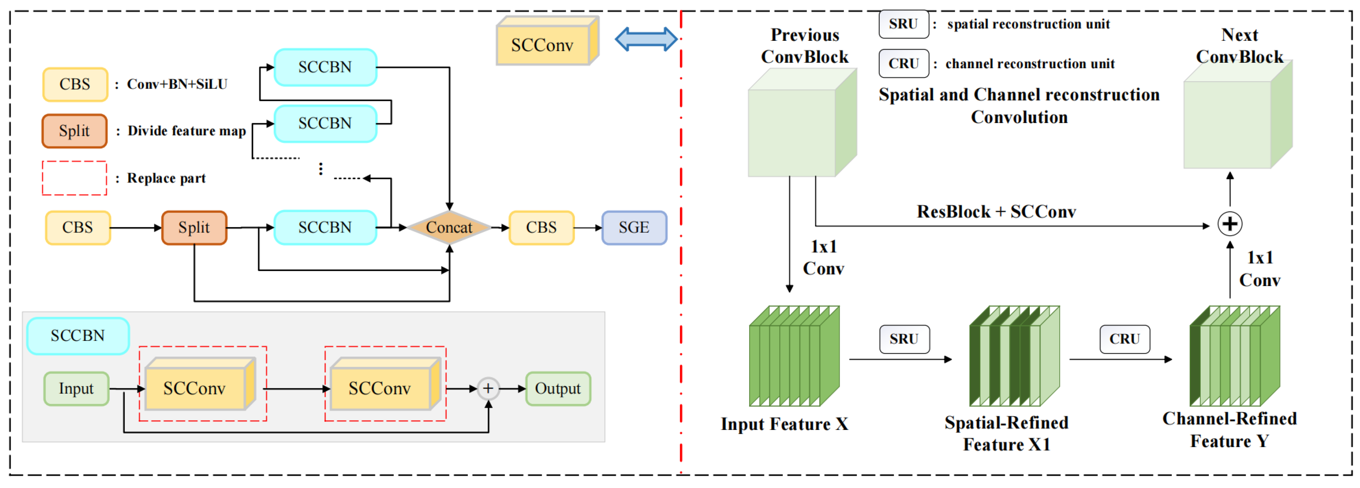
In YOLOv8, the C2f module fuses low-level and high-level feature maps to capture a rich flow of gradient information. However, the Bottleneck module, which contains numerous complex convolutions, significantly increases the model’s parameter size and computational complexity. To address this issue, we propose the SSC2f module, which replaces the Bottleneck with the newly designed SCCBN module. Simultaneously, the SGE attention mechanism is introduced to enhance the model’s accuracy. This is illustrated in Figure 3.
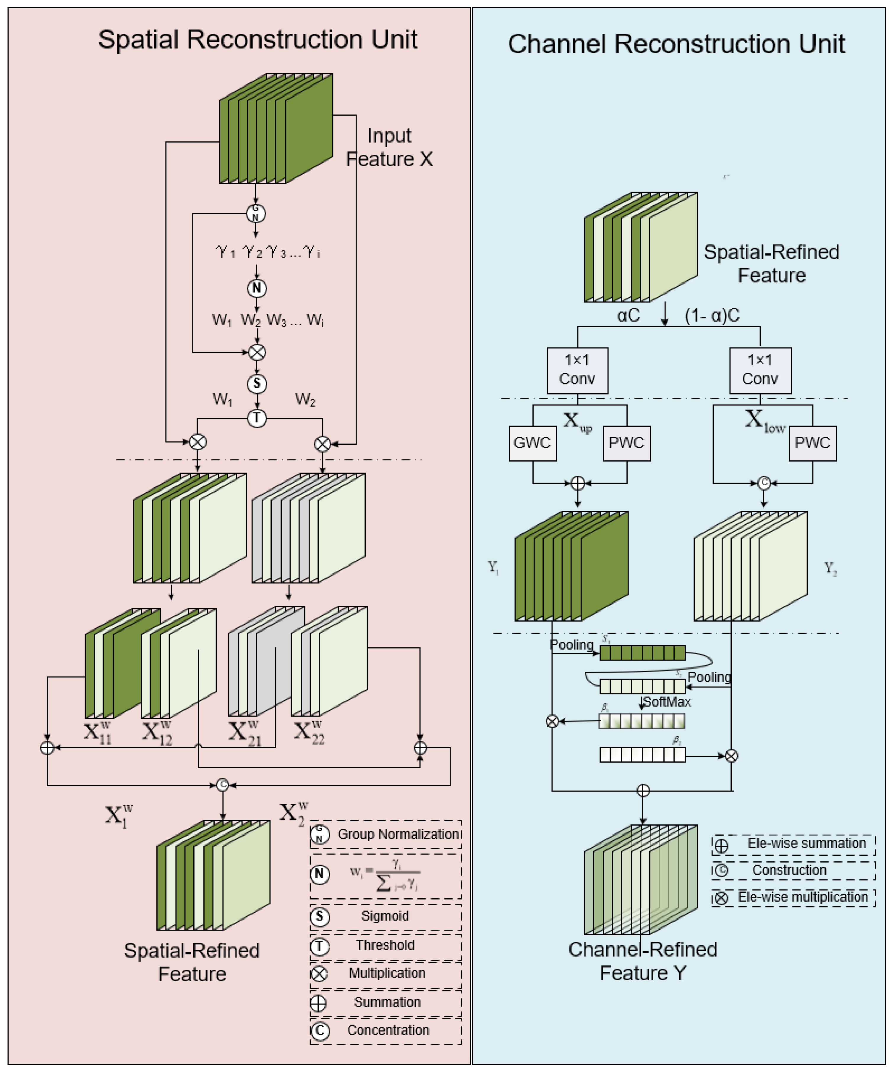
The spatial and channel reconstruction convolution (SCConv) module’s primary role is to reduce spatial and channel redundancy in convolutional neural networks, compressing the CNN model and enhancing its performance. It comprises two units: the spatial reconstruction unit (SRU) and the channel reconstruction unit (CRU). These units work together to decrease computational complexity and lighten the model, as shown in Figure 4.
The SRU module primarily reduces spatial redundancy through a separate reconstruction approach. Initially, the features are normalized using group normalization. Subsequently, trainable parameters, γ, in the GN layer are used to measure the variance of spatial pixels across each batch and channel. The magnitude of γ is associated with the variability in spatial pixels, indicating that a larger γ value corresponds to the model reflecting richer spatial information. The computation formula is indicated by Equation (3):
W γ = { W i } = γ i Σ j = 1 C γ j , I , j = 1 , 2 , , C ,
where W γ R C belongs to the normalized correlation weight.
Upon obtaining the normalized weights, the model maps the range of these weights to the interval (0, 1) using a sigmoid function. Concurrently, the threshold is set at 0.5. Weights above this threshold are assigned a value of 1, forming the information weight W 1 , while those below the threshold are set to 0, resulting in the information weight W 2 .
Subsequently, the input features X are multiplied by W 1 and  W 2 separately, yielding corresponding weighted matrices X W 1 and X W 2 . Here, X W 1 retains the higher information quantity, whereas X W 2  contains the lower information quantity. To enhance information interaction, the model employs a cross-reconstruction operation that effectively combines these two distinct information characteristics. Afterward, the two reconstructed features are concatenated. This entire reconstruction operation can be summarized by Equation (4):
X 1 w = W 1 X , X 2 w = W 2 X , X 11 w X 22 w = X w 1 , X 21 w X 12 w = X w 2 , X w 1 X w 2 = X w ,
where is element-wise multiplication, is element-wise summation, and is concatenation. After applying the spatial reconstruction unit (SRU) to the intermediate input features X, this process not only distinguishes between features with high and low information content, but also strengthens key features while reducing superfluous elements in the spatial dimension.
The channel reconstruction unit (CRU) employs a segment–transform–fuse method to minimize channel redundancy. For the given spatially optimized features, 1 × 1 convolution compresses the channels. The split ratio is determined within the range of (0,1), followed by an aggregation step.
Then, high-efficiency convolution GWC and PWC are used to operate on the features X up , respectively, to extract representative information. Due to the sparse convolution connections in GWC, there is a reduction in parameters and computational load, but it also impedes information exchange between different channel groups. PWC compensates for this loss of information flow and promotes internal channel feature dynamics. Hence, we apply a k × k GWC operation followed by a 1 × 1 PWC operation. After that, the output is added to form a feature, Y 1 , with the following calculation represented by Equation (5):
Y 1 = M G X u p + M P 1 X u p ,
where M G α c g r × k × k × c   and   M P 1 α c r × 1 × 1 × c are learnable weight matrices of GWC and PWC, and X u p   α c r × h × w and Y 1 c × h × w are the upper input and output feature maps, respectively.
Further, a cost-effective 1 × 1 PWC operation is utilized to generate feature maps containing shallow-hidden details, supplementing the rich feature extraction process. Additionally, existing features are reused to generate more feature maps. The resulting features are concatenated with the reused features to obtain the feature Y 2 . Equation (6) is as follows:
Y 2 = M P 2 X low X low ,
where M P 2 1 α c r × 1 × 1 × 1 1 α r c is a learnable weight matrix of PWC, U is a concatenation operation, and X low   1 α c r × h × w and Y 2 c × h × w are the lower input and output feature maps, respectively.
Post-transformation, Y 1 and Y 2 undergo global average pooling to gather global spatial information with channel statistics S m ϵ R C 1 1 . Subsequently, the global channel symbols S 1  and S 2 are stacked, and a channel soft attention operation is used to generate a feature importance vector β 1 , β 2 R c , denoted as Equations (7) and (8):
S m = P o o l i n g Y m = 1 H × W i = 1 H j = 1 W Y c ( i , j ) , m = 1 , 2
β 1 = e s 1 e s 1 + e s 2 , β 2 = e s 2 e s 1 + e s 2 , β 1 + β 2 = 1 .
Finally, under the guidance of the feature importance vector β 1 , β 2 , the channel-refined features Y can be obtained by merging the upper features, Y 1 , and the lower features, Y 2 , in a channel-wise manner.
The SGE (Spatial Group-wise Enhance) attention mechanism is an efficient spatial attention mechanism that enhances the performance of Convolutional Neural Networks (CNNs) in handling image tasks. It selectively groups and encodes information in the feature maps to extract richer and more distinctive feature representations. The calculation process is shown in Figure 5.
Initially, the input feature maps are grouped based on certain criteria (such as channel distribution), so that each group contains a portion of the channels. The statistical characteristics (such as mean or maximum) of each group are independently calculated to reflect the spatial distribution of features within the group. The formula is shown as Equation (9).
g = F g p ( X ) = 1 m i = 1 m x i
Here, g represents the global semantic features and x i represents the local features. Subsequently, a small network is utilized to generate spatial attention maps based on these statistical features, highlighting the importance of features at each position. By element-wise multiplication of the attention map with the original feature map, an importance coefficient for each feature is generated. This dot product measures the similarity between g and x i to a certain extent. Therefore, for each position, the formula is shown as Equation (10).
c i = g x i .
Note that c i can also be expanded as g x i cos θ i , where θ i is the angle between g and x i . As defined by the dot product of vectors, features with larger magnitudes and directions more closely aligned with g are likely to receive larger initial coefficients. To avoid the disparity in coefficient magnitudes across different samples, we implement normalization c across the space. The formula is shown as Equation (11).
c ^ i = c i μ c σ c + ϵ , μ c = 1 m j m c j , σ c 2 = 1 m j m c j μ c 2 ,
where ϵ is a constant added for numerical stability. To ensure the normalization within the network can act as the identity transformation, we introduce a scaling and shifting parameter pair γ , β for each coefficient c ˆ i , modifying the normalized value accordingly. In a single SGE cell, the number of γ , β is the same as the number of groups G, which is of the order of a few tens (typically 32 or 64). It is shown in Equation (12).
a i = γ c ^ i + β
where γ , β are the only parameters introduced in our module. Ultimately, to acquire the improved feature vector x ˆ i , the original x ˆ i is adjusted by the importance coefficients a i generated through a sigmoid function gate σ across the space. The formula is shown as Equation (13).
x ^ i = x i σ a i
And all the enhanced features form the resulting feature group: X ^ = x ^ 1 m , x ^ i C G , m = H × W .

2.3. Optimization of Complex-Scene Recognition

In ship recognition tasks, the accurate identification of ships is affected by the complex maritime environment, which includes varying weather, sea waves, and lighting conditions. The C2f module’s extraction of features from complex backgrounds can lead to feature loss, causing biases in target recognition. Traditional squeeze-and-excitation (SE) attention mechanisms [39] enhance the network’s representativeness and performance by explicitly recalibrating the feature responses of convolutional layers. However, the SE module mainly focuses on the relationships between channels, neglecting the spatial information in feature maps. Therefore, this paper introduces a new lightweight attention module, MC2f, combining the multidimensional collaborative attention (MCA) mechanism to efficiently model spatial and channel features, significantly improving model performance. Its specific structure is shown in Figure 6.
The MCA mechanism primarily consists of three parallel branches, with the first two focusing on capturing spatial feature dependencies W and H, and the last one emphasizing the interactions between channels.
In the first branch, the output feature map F from the convolutional layer is initially rotated 90° counterclockwise along the H-axis, generating a rotated feature map F ^ W . This map is then fed into a Squeeze Transformation module, which models both channel (C) and spatial (H) dimensions to produce an aggregated feature map. Subsequently, this aggregated map,  F ˆ W ,  undergoes processing via an Excitation Transformation module to capture interactions among spatial dimensions and generate attention weights using a sigmoid function. These attention weights are applied to the rotated feature map through element-wise multiplication, resulting in an enhanced feature map, F w . Finally, the enhanced feature map is rotated back 90° clockwise to its original orientation. This process can be summarized by Equations (14)–(16):
F ^ W = P M H ( F )
F ^ W = T s q ( F ^ W ) , F ˜ W = T e x ( F ^ W )
A W = σ ( F ˜ W ) , F W = A W F ^ W , F W = P M H 1 ( F W ) ,
where P M H denotes rotation through 90 anti-clockwise along the H -axis, while P M H 1 denotes the inverse, both of which can be easily implemented by the permute operation in the PyTorch toolbox. σ stands for the sigmoid activation function. T s q and T e x refer to the squeeze transformation and excitation transformation, respectively.
Similarly, the second branch initiates a counterclockwise rotation of the feature map F by 90° along the W-axis, resulting in the rotated feature map denoted as F ^ H . To model interactions among height dimensions effectively, consecutive Squeeze Transformation and Squeeze Transformation operations are applied to capture both channel dimension C and spatial dimension H. This process generates aggregated feature maps, F ˆ H , and height feature weights, F ˜ H . Subsequently, attention weights are obtained through the sigmoid function, and these weights undergo element-wise multiplication with the initial features, yielding the enhanced feature map,   F H . Finally, a 90° clockwise rotation along the W-axis is performed, restoring the shape to be identical to the original input. This entire procedure is succinctly represented by Equations (17)–(19):
F ^ H = P M W F
F ^ H = T s q F ^ H , F ˜ H = T e x F ^ H
A H = σ F ˜ H , F H = A H F ^ H , F H = P M W 1 F H .
The lower branch is primarily designed to model spatial dependencies and capture interactions among channels. It starts by generating feature maps that are identical via identity mapping. These feature maps are then sequentially processed through two modules, namely Squeeze Transformation and Excitation Transformation. This sequential processing allows for the inference of aggregated feature maps and channel feature weights. Subsequently, attention weights are derived using the sigmoid function. The original features are then rescaled based on these attention weights, resulting in enhanced feature maps. Finally, a feature mapping function is applied. Similarly, this entire process is represented by Equations (20) and (21).
F ^ C = T s q F ^ C , F ˜ C = T e x F ^ C
A C = σ F ˜ C , F C = A C F ^ C , F C = I M F C ,
where I M · refers to the identity mapping function.
Finally, an integration operation is applied to consolidate the features generated by the three branches. This process ensures that the resulting features achieve more accurate localization of relevant details, thereby enhancing overall discernibility, as illustrated by Equation (22):
F = 1 3 ( F W F H F C )
Here, F W , F H , and F C can be represented by Formula Group (23):
F W = P M H 1 σ T e x T s q P M H F P M H F F H = P M W 1 σ T e x T s q P M W F P M W F F C = I M σ T e x T s q I M F I M F .

2.4. Optimization of Multi-Scale Target Recognition Accuracy

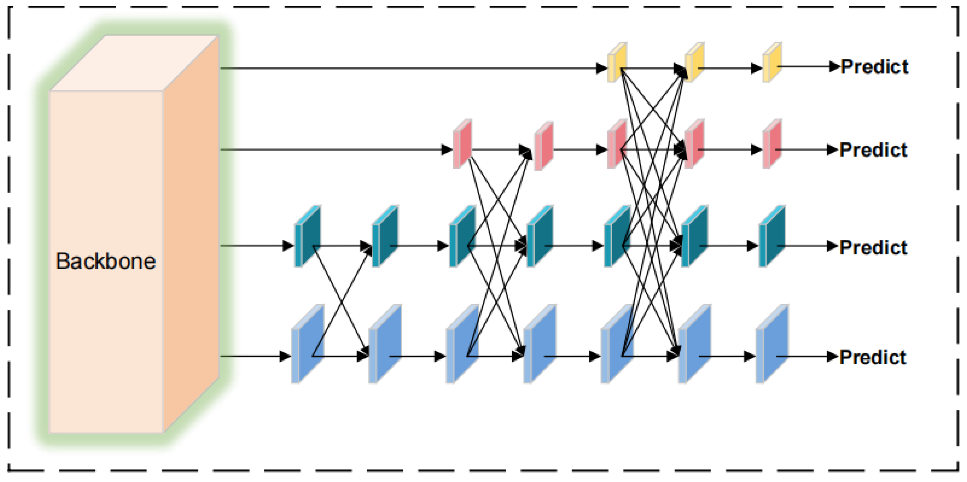
In ship recognition tasks, the varying distance and size of ships, causing inconsistent target scales, can impede a model’s feature extraction capability. YOLOv8n primarily employs FPN + PAN for feature fusion, yet its effectiveness in detecting targets of extreme scales is relatively limited. Moreover, excessive fusion might lead to feature confusion. To address this issue, this study utilized the AFPN structure to filter features during the multi-level fusion process, effectively mitigating the contradictions between features at different levels. The specific architecture of AFPN is illustrated in Figure 7.
Before features fusion, it is essential to extract distinct features from the backbone. Following the design of the Faster R-CNN framework, the last layer of features is extracted from each feature level of the Backbone. These varying scale features are represented as {C2, C3, C4, C5}. For feature fusion, the lower-level features C2 and C3 are initially fed into a feature pyramid network. Subsequently, C4 and C5 are fused. Upon completion of the fusion process, a series of feature sets of different scales, including P2, P3, P4, and P5, are generated.
Next, the extracted features undergo feature fusion. The semantic disparity between non-adjacent layer features extracted by the backbone network is significantly greater than that between adjacent layers. Direct fusion could lead to a poor integration of non-adjacent layer features. Therefore, the AFPN adopts a progressive integration structure. It first fuses primary features, then intermediate features, and finally advanced features. This ensures that different levels of information are more semantically aligned in the gradual fusion process.
After fusing the features, an adaptive spatial fusion operation is necessary. Thus, by employing the adaptive spatial feature fusion (ASFF) technique, different spatial weights are assigned to the features at each level. This approach strengthens the role of key levels while minimizing the impact of conflicting information arising from different targets. The specific implementation details are outlined in Equation (24):
y i j l = α i j l x i j 1 l + β i j l x i j 2 l + γ i j l x i j 3 l ,
where α i j l , β i j l , and γ i j l represent the spatial weights of the features of the three levels at level l , subject to the constraint that α i j l + β i j l + γ i j l = 1 .

3. Results

3.1. Dataset

Ship detection in images holds significant practical value, playing a crucial role in ensuring maritime traffic safety, enhancing surveillance efficiency, and optimizing marine resource management.
The experiments in this paper utilized remote sensing aerial data from the Ships dataset [40]. A total of 9697 aerial and satellite images were collected from the Ships dataset, with each image sized at 768 × 768. These images are annotated with bounding boxes in the YOLO format, allowing for an accurate and effective detection of ships within the images. The dataset contains only one category: ships. It is divided into training, validation, and test sets in an 8:1:1 ratio. Images were sourced from various maritime areas, including busy harbors, open seas, and coastal regions, showcasing a range of vessels from small fishing boats to large cargo ships, ensuring broad coverage across different marine environments and types of ships. The paper presents the selected centroid coordinates and dimensions, as shown in Figure 8.

3.2. Environment and Evaluation

This experiment was conducted on a Windows 10 operating system, utilizing version 2.0 of the PyTorch framework. Additionally, the experiment was equipped with an NVIDIA RTX 3090 graphics card with 24 GB of VRAM, ensuring ample graphics processing capacity. To maintain consistency in the experimental process and comparability of the results, this experimental setup will remain unchanged in subsequent sections.
To comprehensively assess the model proposed in this study, this paper employed several quantitative evaluation metrics, including Recall, Precision, F1, and mAP.
(1)
TP, FP, TN, FN
TP (true positive) refers to the number of instances where the model correctly identifies positive-class samples as positive. FP (false positive) denotes the number of instances where the model incorrectly identifies negative-class samples as positive. TN (true negatives) represents the number of instances where the model correctly identifies negative-class samples as negative. FN (false negatives) indicates the number of instances where the model incorrectly classifies positive-class samples as negative.
(2)
Recall and Precision
Recall measures the proportion of correctly identified positive samples by a model out of all actual positive samples, calculated employing Equation (25):
R e c a l l = T P T P + F N
Precision measures the proportion of samples predicted as positive by a model that is actually positive. The calculation formula is shown by Equation (26):
P r e c i s i o n = T P T P + F P
(3)
F1
The F1 score is the harmonic mean of precision and recall, used to comprehensively evaluate a model’s accuracy and completeness. The calculation formula is shown by Equation (27):
F 1 = 2 × P r e c i s i o n × R e c a l l P r e c i s i o n + R e c a l l
(4)
AP and mAP
AP (average precision) is a metric used to evaluate the performance of an object detection model on a specific class. It reflects the balance between precision and recall, which is the average performance value on the precision–recall curve. Its calculation formula is shown by Equation (28):
A P = i = 1 n P i Δ r i = 0 1 p r d r
mAP (mean average precision) is a metric derived by averaging the average precision (AP) across multiple classes. It is used to measure the overall performance of a detection model across the entire dataset. Its calculation formula is shown by Equation (29):
m A P = n = 1 N A P n N
(5)
Weights, parameters, and FLOPs
Weights are the crucial trainable parameters in a neural network responsible for adjusting the model’s performance of specific tasks, such as object detection. “Parameter count” represents the total number of parameters in the model, including weights and biases, and is a significant metric for assessing the network’s size and complexity, directly impacting its computational and storage requirements. Additionally, FLOPs (floating-point operations per second) is a key metric for measuring computational load. It is typically used to indicate the number of floating-point operations required for one forward pass of the model, which is essential for understanding the model’s computational efficiency.

3.3. Experimental Result

3.3.1. Comparative Experiment after Model Optimization

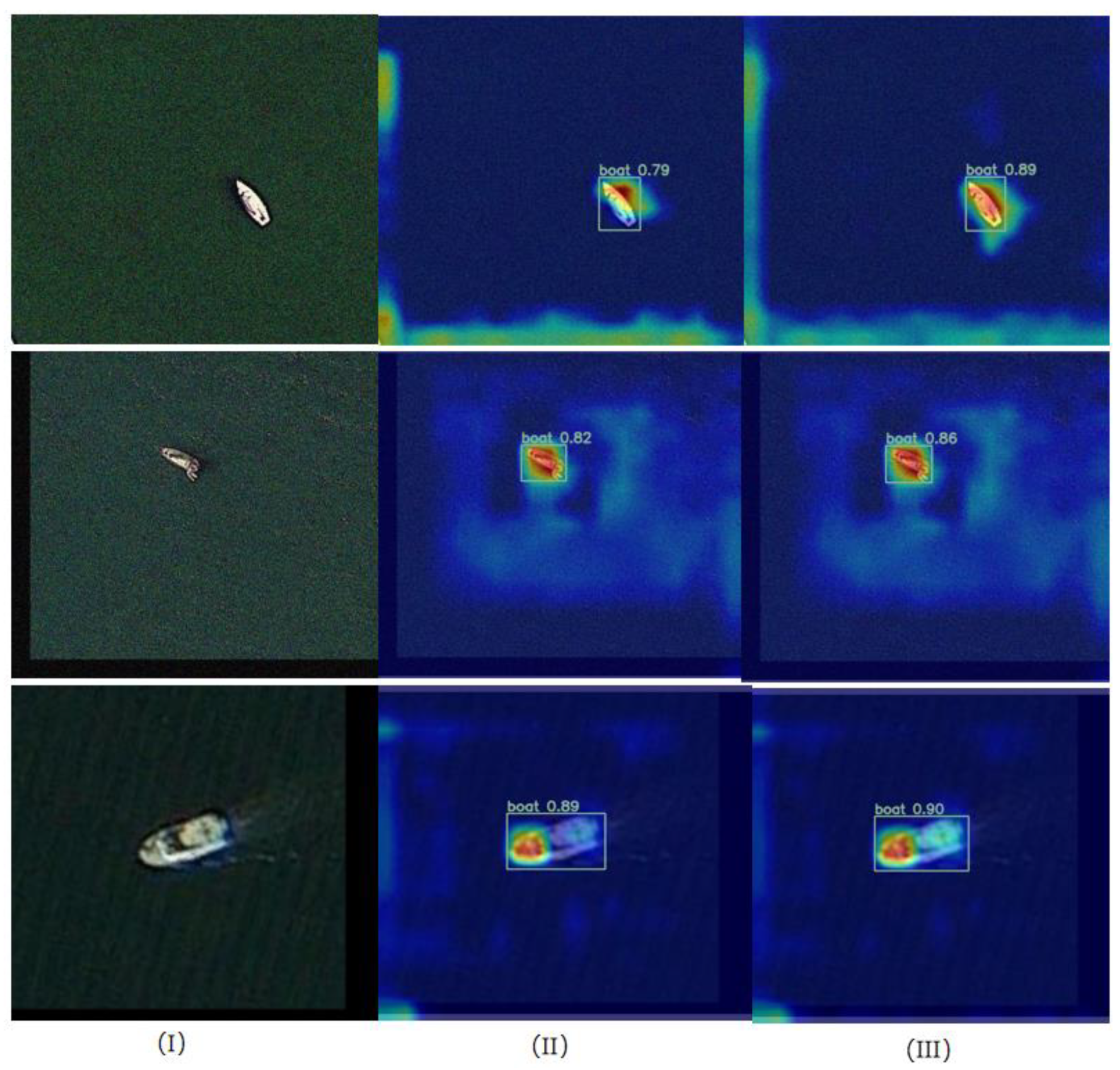
We employ Grad-CAM for interpretability analysis of the model improvement strategy. Figure 9 displays the effects of target detection on the Ships dataset as obtained by Grad-CAM for YOLOv8n and SSMA-YOLO. It is observable that, compared to YOLOv8n, SSMA-YOLO has a higher focus on target areas for detecting the location of the object, while paying less attention to irrelevant environmental information in non-target areas.
To confirm the superiority of the SSMA-YOLO model proposed in this study for remote sensing ship detection tasks compared to the YOLOv8n model, the authors of this paper conducted comparative experiments under the same conditions to assess the performance of both models. The results are shown in Table 1.
Table 1 clearly demonstrates that our proposed SSMA-YOLO model surpasses the YOLOv8n model in performance when tested employing identical datasets and experimental conditions. The SSMA-YOLO model achieves notable advancements over the standard YOLOv8n baseline in Precision, Recall, F1, and mAP by margins of 3.2%, 4.8%, 4.2%, and 4.4%, respectively. These improvements largely stem from the integration of the optimized MC2f structure, which enhances the model’s capacity for extracting information from complex backgrounds. Additionally, the AFPN structure in the feature fusion process significantly raises the model’s accuracy in detecting targets across different scales. Moreover, a reduction in model parameters by 23% is achieved through the incorporation of the lightweight GhostConv and the innovative SSC2f module, elevating computational efficiency by streamlining the convolution process and minimizing redundancy in space and channels.
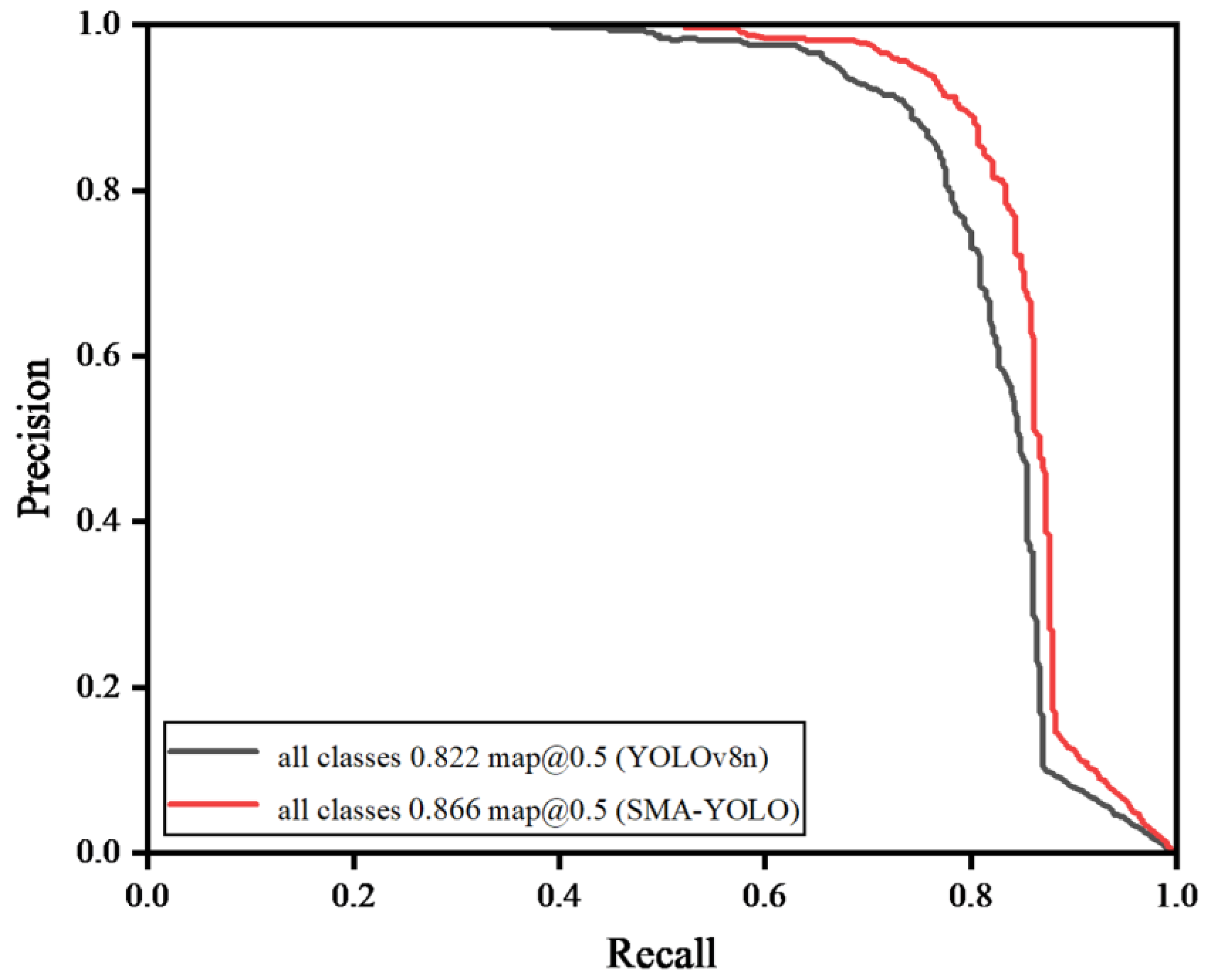
The P–R curve, revealing the Precision and Recall relationship across various thresholds, indicates that a larger curve area, representing a higher AP, correlates with improved model performance. The SSMA-YOLO model, as shown in Figure 10, encloses a larger P–R curve area (0.866) compared to YOLOv8n (0.822), confirming the enhanced detection capabilities of our refined model over the original YOLOv8n.
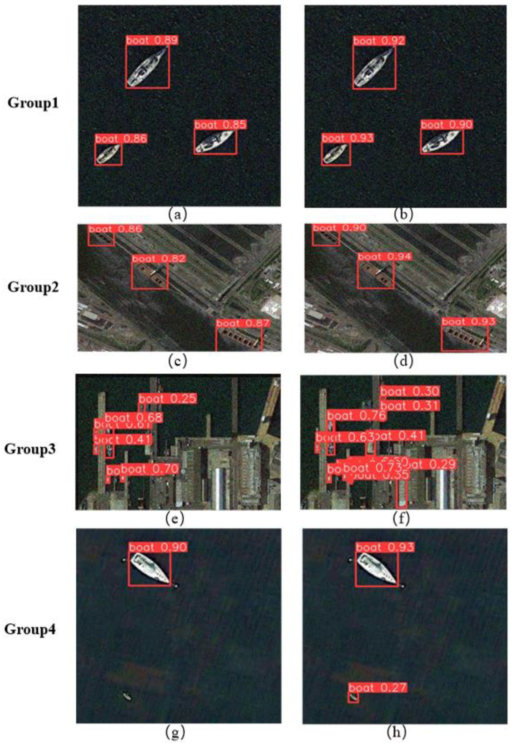
Figure 11 presents a comparison of the SSMA-YOLO and YOLOv8n models in detecting various maritime scenarios and targets. Group 1 showcases the detection accuracy under normal conditions, with Figure 11a,b demonstrating that the SSMA-YOLO model consistently achieves higher detection precision than the YOLOv8n model. Group 2 represents detection in dense ship scenarios, where Figure 11c,d illustrate that SSMA-YOLO exhibits superior detection accuracy in crowded maritime environments. Group 3, concerning ship detection against complex backgrounds, shows from Figure 11e,f that the SSMA-YOLO model not only achieves higher accuracy but also detects more ships that YOLOv8n fails to identify. Group 4 covers multi-scale target detection scenarios; Figure 11g,h indicate that while YOLOv8n primarily focuses on conventional scales, neglecting smaller targets, SSMA-YOLO maintains high precision for standard-sized ships and effectively detects smaller targets. In conclusion, the SSMA-YOLO model exhibits superior ship detection performance compared to the YOLOv8n model.

3.3.2. Ablation Experiment

Based on Table 2, it is evident that each integration of a new module optimizes the model’s performance. Compared to YOLOv8n, YOLOv8n + SSC2f shows an 16% reduction in computational load, albeit with a slight decrease in detection accuracy. This is because the use of the Ghostconv and SSC2f lightweight model structures somewhat reduces the network’s depth and width, potentially diminishing the model’s ability to capture complex features, leading to a decreased detection accuracy. However, when compared to YOLOv8n + SSC2f, YOLOv8n + SSC2f + MC2f shows improvements of 3.2%, 4.3%, 3.4%, and 2.1% in Precision, Recall, F1, and mAP, respectively, while maintaining a similar computational load to YOLOv8n + SSC2f. This improvement is attributed to the introduction of the MC2f module, which efficiently captures spatial and channel features, significantly enhancing the model’s performance in processing images with complex backgrounds while maintaining its lightweight nature. Moreover, the YOLOv8n + SSC2f + MC2f + AFPN structure, compared to YOLOv8n + SSC2f + MC2f, achieves increases of 2.1%, 1.2%, 1.7%, and 2.3% in Precision, Recall, F1, and mAP, respectively. This enhancement is due to the added AFPN module, which filters features in multi-level fusion processes, mitigating the contradiction of information among different feature levels, effectively strengthening the model’s ability to recognize images of varying scales, and thus significantly improving its overall performance metrics.

3.3.3. Comparison with Other Models

To further validate the effectiveness of the SSMA-YOLO algorithm, it was compared with popular object detection algorithms such as Faster R-CNN, SSD, YOLOv3, YOLOv5, and YOLOv7. To ensure fairness in the experiments, all algorithms were trained with identical parameter settings, including a fixed number of training iterations set to 300. The results of the comparative experiments are shown in Table 3.
As indicated by Table 3, the SSMA-YOLO algorithm designed in this study exhibits superior detection accuracy compared to other object detection algorithms. Faster-RCNN [41] achieves high detection accuracy by first generating potential target regions and then performing classification and bounding box regression on these regions. However, due to its complex model framework, it struggles to meet real-time detection requirements. SSD [42], a single-stage detection algorithm, uses multi-scale feature maps to detect objects, offering improvements in detection speed and performance over Faster-RCNN. However, this method is sensitive to noise and variations in input images, which may lead to unstable detection results. Utilizing a fully convolutional network, YOLOv3 [43] provides better detection accuracy, but its large model size limits its practical application. YOLOv5 [44] improves detection performance through enhanced network structures and more advanced feature extraction techniques. However, it requires a large amount of training data and its training complexity is high, leading to model instability. The YOLOv7 [45] algorithm enhances detection performance through more efficient convolution operations and a smaller model structure. Within the range of 5 FPS to 160 FPS, it surpasses most object detectors in both speed and accuracy and holds the highest AP accuracy of 56.8% among all known real-time object detectors with 30 FPS or higher on a GPU V100. However, its approach of dividing images into fixed-size grids may limit the algorithm’s versatility. This design may lead to inconsistent performance when processing diverse datasets and scenarios, affecting its generalizability. Experimental results show that SSMA-YOLO demonstrates exceptional performance, significantly reducing the model’s parameter count and clearly outperforming other object detection models in various performance metrics. Compared to YOLOv7, YOLOv5, and YOLOv3 from the same series, the SSMA-YOLO algorithm exhibits increases in the mAP metric of 4.0%, 5.1%, and 6.2%, respectively.

3.3.4. Generalization Test

As ship detection often encounters various scenarios, to further evaluate the performance of the model proposed in this paper, it has been validated on the SSDD dataset [46] and the HRSC-2016 dataset [47]. The SSDD is specifically designed for ship detection in satellite imagery, comprising 1160 high-resolution remote sensing images. It is divided into training, validation, and test sets in an 8:1:1 ratio, containing a single category: ship. The HRSC2016 dataset focuses on ship target detection in the field of remote sensing imagery. This dataset includes high-resolution remote sensing images, showcasing a variety of ship types and sizes. It consists of 1170 remote sensing ship images, also with just the ship category. The dataset division follows the same 8:1:1 ratio. Experiments conducted on these two datasets serve to further validate the effectiveness of the model under discussion. The experimental results are shown in Table 4.
The SSMA-YOLO model proposed in this paper demonstrates higher performance compared to mainstream object detection models on two different datasets, as evident from Table 4. This further confirms the superiority of the SSMA-YOLO model introduced in our study.

4. Discussion

To address issues such as maritime traffic safety, which are impacted by inaccurate or untimely ship recognition, this paper introduces the SSMA-YOLO model. This model significantly improves ship detection performance in complex sea surface backgrounds and varying target sizes. Additionally, its lightweight structure facilitates real-time detection tasks.
First, addressing the real-time detection needs in ship recognition, the main challenge faced in current research is the excessive complexity of most model structures, hindering swift processing. This paper introduces a newly designed SSC2f module, combined with the lightweight GhostConv convolution, to achieve a lightweight YOLOv8n model. This design effectively reduces spatial and channel redundancy in convolutional neural networks, significantly lowering the model’s parameter count, thereby enhancing its real-time detection performance. Additionally, the paper redesigned the MC2f module, which models spatial and channel features efficiently through three parallel branches, enhancing the model’s ability to accurately locate and identify the details of interest. This improvement significantly increased the model’s accuracy in recognizing ships against complex backgrounds. Lastly, the paper employed the AFPN structure to optimize the multi-level feature fusion process. This structure effectively mitigates information conflicts between different levels of features, strengthening the fusion effect and thus enhancing the model’s capability to detect ship images of various scales.
In comparison with other methods in the same field, traditional ship detection primarily relies on manual monitoring. However, this approach faces significant limitations in terms of coverage area, continuous monitoring capability, and efficiency. Moreover, prolonged continuous work can lead to operator fatigue, thereby increasing safety risks. Additionally, deep learning-based object detection methods are categorized as being two-stage and one-stage. The two-stage object detection algorithm is inefficient in the process of generating region recommendations and performing bounding box regression, and consumes a large amount of computing resources, which is not conducive to real-time detection tasks. On the other hand, current one-stage object detection algorithms can directly predict bounding boxes and class probabilities from a complete image in a single evaluation, significantly increasing speed. However, existing one-stage algorithms perform poorly when dealing with densely packed ships and varying target sizes. In this paper, the SSMA-YOLO model proposed significantly enhanced the performance of ship recognition with complex backgrounds and complex-scale scenarios, while maintaining lightweight design, through the incorporation of the MC2f module and the integration of the AFPN structure.
However, the model designed in this paper still has certain limitations. The dataset used in this study may not cover all complex scenarios, such as ship images in different maritime areas under conditions such as heavy fog and low light, which could result in poor model generalizability to specific situations. Additionally, while the AFPN structure employed in this paper allows for the acquisition of richer features, dealing with and fusing multi-level feature maps requires a deeper network structure, leading to increased computational complexity.

5. Conclusions

Ship recognition plays a crucial role in ensuring maritime traffic safety and the effective management of ocean resources. This paper introduced a single-stage ship target detection model that enhances detection performance. Utilizing the newly designed SSC2f module, the network structure was made lightweight, significantly reducing the model’s parameters. Additionally, the newly proposed MC2f module addresses the issue of low accuracy in complex-scene recognition. Lastly, the AFPN structure progressively fuses features at different levels, effectively solving the problem of low multi-scale target recognition accuracy during ship recognition tasks. However, from the perspective of attention mechanisms, the model only considered spatial features from two directions, while still lacking the ability to focus on targets effectively. By modeling spatial features from more directions, the model was able to more accurately recognize and locate targets, especially in scenarios with complex backgrounds or where targets varied greatly in shape and size. Simultaneously, this meant the model could capture information across more dimensions, which is particularly crucial for understanding a target’s three-dimensional structure, orientation, and spatial relationship with other objects.
Future research will focus on gathering and analyzing image data captured under extreme weather conditions to enhance the model’s generalization capability across various environments. To address the issue of increased computational complexity caused by the AFPN structure, future studies should emphasize the design of more compact and efficient network architectures, such as depth-wise separable convolutions, to reduce computational complexity and memory requirements, enabling more efficient applications in real-time detection tasks. Additionally, future efforts will optimize the attention mechanism, considering spatial features from more directions, to further enhance the model’s detection accuracy.

Author Contributions

Conceptualization, Y.H. and T.Z.; methodology, Y.H.; software, Y.H.; validation, Y.H., T.Z. and J.G.; formal analysis, Y.H., J.G. and H.Y.; investigation, Y.H. and J.G.; data curation, Y.H., J.G. and H.Y.; writing—original draft preparation, Y.H.; writing—review and editing, Y.H., J.G., R.G. and H.Y.; visualization, Y.H., R.G., J.G. and H.Y.; supervision, Y.H. and T.Z.; project administration, Y.H. All authors have read and agreed to the published version of the manuscript.

Funding

This research received no external funding.

Data Availability Statement

The datasets involved in the article are available on request from the first author.

Conflicts of Interest

The authors declare no conflicts of interest.

References

  1. Arivazhagan, S.; Lilly Jebarani, W.S.; Newlin Shebiah, R.; Ligi, S.V.; Hareesh Kumar, P.V.; Anilkumar, K. Significance Based Ship Detection from SAR Imagery. In Proceedings of the 2019 1st International Conference on Innovations in Information and Communication Technology (ICIICT), Chennai, India, 25–26 April 2019; pp. 1–5. [Google Scholar]
  2. Dominguez-Péry, C.; Tassabehji, R.; Corset, F.; Chreim, Z. A Holistic View of Maritime Navigation Accidents and Risk Indicators: Examining IMO Reports from 2011 to 2021. J. Shipp. Trade 2023, 8, 11. [Google Scholar] [CrossRef]
  3. Goerlandt, F.; Goite, H.; Banda, O.A.V.; Höglund, A.; Ahonen-Rainio, P.; Lensu, M. An Analysis of Wintertime Navigational Accidents in the Northern Baltic Sea. Saf. Sci. 2017, 92, 66–84. [Google Scholar] [CrossRef]
  4. Goerlandt, F.; Montewka, J. Maritime Transportation Risk Analysis: Review and Analysis in Light of Some Foundational Issues. Reliab. Eng. Syst. Saf. 2015, 138, 115–134. [Google Scholar] [CrossRef]
  5. Teixeira, E.; Araujo, B.; Costa, V.; Mafra, S.; Figueiredo, F. Literature Review on Ship Localization, Classification, and Detection Methods Based on Optical Sensors and Neural Networks. Sensors 2022, 22, 6879. [Google Scholar] [CrossRef] [PubMed]
  6. Crow’s Nest. Wikipedia 2023. Available online: https://en.wikipedia.org/w/index.php?title=Crow%27s_nest&oldid=1186905465 (accessed on 6 April 2024).
  7. Lu, Z.; Wang, P.; Li, Y.; Ding, B. A New Deep Neural Network Based on SwinT-FRM-ShipNet for SAR Ship Detection in Complex Near-Shore and Offshore Environments. Remote Sens. 2023, 15, 5780. [Google Scholar] [CrossRef]
  8. Tian, Y.; Wang, X.; Zhu, S.; Xu, F.; Liu, J. LMSD-Net: A Lightweight and High-Performance Ship Detection Network for Optical Remote Sensing Images. Remote Sens. 2023, 15, 4358. [Google Scholar] [CrossRef]
  9. Yasir, M.; Niang, A.J.; Hossain, M.S.; Islam, Q.U.; Yang, Q.; Yin, Y. Ranking Ship Detection Methods Using SAR Images Based on Machine Learning and Artificial Intelligence. J. Mar. Sci. Eng. 2023, 11, 1916. [Google Scholar] [CrossRef]
  10. Cao, X.; Gao, S.; Chen, L.; Wang, Y. Ship Recognition Method Combined with Image Segmentation and Deep Learning Feature Extraction in Video Surveillance. Multimed. Tools Appl. 2020, 79, 9177–9192. [Google Scholar] [CrossRef]
  11. Xing, X.; Ji, K.; Zou, H.; Sun, J. Feature Selection and Weighted SVM Classifier-Based Ship Detection in PolSAR Imagery. Int. J. Remote Sens. 2013, 34, 7925–7944. [Google Scholar] [CrossRef]
  12. He, J.; Hao, Y.; Wang, X. An Interpretable Aid Decision-Making Model for Flag State Control Ship Detention Based on SMOTE and XGBoost. J. Mar. Sci. Eng. 2021, 9, 156. [Google Scholar] [CrossRef]
  13. Yan, Z.; Song, X.; Yang, L.; Wang, Y. Ship Classification in Synthetic Aperture Radar Images Based on Multiple Classifiers Ensemble Learning and Automatic Identification System Data Transfer Learning. Remote Sens. 2022, 14, 5288. [Google Scholar] [CrossRef]
  14. Zhao, Z.-Q.; Zheng, P.; Xu, S.; Wu, X. Object Detection with Deep Learning: A Review. IEEE Trans. Neural Netw. Learn. Syst. 2019, 30, 3212–3232. [Google Scholar] [CrossRef]
  15. Chen, C.; Zheng, Z.; Xu, T.; Guo, S.; Feng, S.; Yao, W.; Lan, Y. YOLO-Based UAV Technology: A Review of the Research and Its Applications. Drones 2023, 7, 190. [Google Scholar] [CrossRef]
  16. Liu, J.; Guan, R.; Li, Z.; Zhang, J.; Hu, Y.; Wang, X. Adaptive Multi-Feature Fusion Graph Convolutional Network for Hyperspectral Image Classification. Remote Sens. 2023, 15, 5483. [Google Scholar] [CrossRef]
  17. Guan, R.; Li, Z.; Li, T.; Li, X.; Yang, J.; Chen, W. Classification of Heterogeneous Mining Areas Based on ResCapsNet and Gaofen-5 Imagery. Remote Sens. 2022, 14, 3216. [Google Scholar] [CrossRef]
  18. Guan, R.; Li, Z.; Tu, W.; Wang, J.; Liu, Y.; Li, X.; Tang, C.; Feng, R. Contrastive Multi-View Subspace Clustering of Hyperspectral Images Based on Graph Convolutional Networks. IEEE Trans. Geosci. Remote Sens. 2024, 62, 5510514. [Google Scholar] [CrossRef]
  19. Guan, R.; Li, Z.; Li, X.; Tang, C. Pixel-Superpixel Contrastive Learning and Pseudo-Label Correction for Hyperspectral Image Clustering. In Proceedings of the ICASSP 2024-2024 IEEE International Conference on Acoustics, Speech and Signal Processing (ICASSP), Seoul, Republic of Korea, 14–19 April 2024; IEEE: New York, NY, USA, 2024; pp. 6795–6799. [Google Scholar]
  20. Han, X.; Zhao, L.; Ning, Y.; Hu, J. ShipYolo: An Enhanced Model for Ship Detection. J. Adv. Transp. 2021, 2021, 1060182. [Google Scholar] [CrossRef]
  21. Kouvaras, L.; Petropoulos, G.P. A Novel Technique Based on Machine Learning for Detecting and Segmenting Trees in Very High Resolution Digital Images from Unmanned Aerial Vehicles. Drones 2024, 8, 43. [Google Scholar] [CrossRef]
  22. Zhang, Z. Drone-YOLO: An Efficient Neural Network Method for Target Detection in Drone Images. Drones 2023, 7, 526. [Google Scholar] [CrossRef]
  23. Girshick, R.; Donahue, J.; Darrell, T.; Malik, J. Region-Based Convolutional Networks for Accurate Object Detection and Segmentation. IEEE Trans. Pattern Anal. Mach. Intell. 2015, 38, 142–158. [Google Scholar] [CrossRef]
  24. Li, Y.; Zhang, S.; Wang, W.-Q. A Lightweight Faster R-CNN for Ship Detection in SAR Images. IEEE Geosci. Remote Sens. Lett. 2020, 19, 4006105. [Google Scholar] [CrossRef]
  25. Jiao, J.; Zhang, Y.; Sun, H.; Yang, X.; Gao, X.; Hong, W.; Fu, K.; Sun, X. A Densely Connected End-to-End Neural Network for Multiscale and Multiscene SAR Ship Detection. IEEE Access 2018, 6, 20881–20892. [Google Scholar] [CrossRef]
  26. Zhou, Y.; Jiang, W.; Jiang, X.; Chen, L.; Liu, X. CamoNet: A Target Camouflage Network for Remote Sensing Images Based on Adversarial Attack. Remote Sens. 2023, 15, 5131. [Google Scholar] [CrossRef]
  27. Yu, M.; Han, S.; Wang, T.; Wang, H. An Approach to Accurate Ship Image Recognition in a Complex Maritime Transportation Environment. J. Mar. Sci. Eng. 2022, 10, 1903. [Google Scholar] [CrossRef]
  28. Yu, L.; Wu, H.; Zhong, Z.; Zheng, L.; Deng, Q.; Hu, H. TWC-Net: A SAR Ship Detection Using Two-Way Convolution and Multiscale Feature Mapping. Remote Sens. 2021, 13, 2558. [Google Scholar] [CrossRef]
  29. Redmon, J.; Divvala, S.; Girshick, R.; Farhadi, A. You Only Look Once: Unified, Real-Time Object Detection. In Proceedings of the IEEE Conference on Computer Vision and Pattern Recognition, Las Vegas, NV, USA, 27–30 June 2016. [Google Scholar]
  30. Tang, G.; Liu, S.; Fujino, I.; Claramunt, C.; Wang, Y.; Men, S. H-YOLO: A Single-Shot Ship Detection Approach Based on Region of Interest Preselected Network. Remote Sens. 2020, 12, 4192. [Google Scholar] [CrossRef]
  31. Jiang, J.; Fu, X.; Qin, R.; Wang, X.; Ma, Z. High-Speed Lightweight Ship Detection Algorithm Based on YOLO-v4 for Three-Channels RGB SAR Image. Remote Sens. 2021, 13, 1909. [Google Scholar] [CrossRef]
  32. Xu, X.; Zhang, X.; Zhang, T. Lite-Yolov5: A Lightweight Deep Learning Detector for on-Board Ship Detection in Large-Scene Sentinel-1 Sar Images. Remote Sens. 2022, 14, 1018. [Google Scholar] [CrossRef]
  33. Chen, Z.; Liu, C.; Filaretov, V.F.; Yukhimets, D.A. Multi-Scale Ship Detection Algorithm Based on YOLOv7 for Complex Scene SAR Images. Remote Sens. 2023, 15, 2071. [Google Scholar] [CrossRef]
  34. Zhao, X.; Song, Y. Improved Ship Detection with YOLOv8 Enhanced with MobileViT and GSConv. Electronics 2023, 12, 4666. [Google Scholar] [CrossRef]
  35. Liang, H.; Lee, S.-C.; Seo, S. UAV-Based Low Altitude Remote Sensing for Concrete Bridge Multi-Category Damage Automatic Detection System. Drones 2023, 7, 386. [Google Scholar] [CrossRef]
  36. Li, X.; Zhu, R.; Yu, X.; Wang, X. High-Performance Detection-Based Tracker for Multiple Object Tracking in UAVs. Drones 2023, 7, 681. [Google Scholar] [CrossRef]
  37. GitHub-Ultralytics/Ultralytics: NEW-YOLOv8 🚀 in PyTorch > ONNX > OpenVINO > CoreML > TFLite. Available online: https://github.com/ultralytics/ultralytics (accessed on 16 January 2024).
  38. Ge, Z.; Liu, S.; Wang, F.; Li, Z.; Sun, J. YOLOX: Exceeding YOLO Series in 2021. arXiv 2021, arXiv:2107.08430. [Google Scholar]
  39. Hu, J.; Shen, L.; Sun, G. Squeeze-and-Excitation Networks. In Proceedings of the IEEE Conference on Computer Vision and Pattern Recognition, Salt Lake City, UT, USA, 18–23 June 2018; pp. 7132–7141. [Google Scholar]
  40. Ships/Vessels in Aerial Images. Available online: https://www.kaggle.com/datasets/siddharthkumarsah/ships-in-aerial-images (accessed on 16 January 2024).
  41. Ren, S.; He, K.; Girshick, R.; Sun, J. Faster R-Cnn: Towards Real-Time Object Detection with Region Proposal Networks. IEEE Trans. Pattern Anal. Mach. Intell. 2016, 39, 1137–1149. [Google Scholar] [CrossRef] [PubMed]
  42. Liu, W.; Anguelov, D.; Erhan, D.; Szegedy, C.; Reed, S.; Fu, C.-Y.; Berg, A.C. SSD: Single Shot MultiBox Detector. In Computer Vision–ECCV 2016; Leibe, B., Matas, J., Sebe, N., Welling, M., Eds.; Lecture Notes in Computer Science; Springer International Publishing: Cham, Switzerland, 2016; Volume 9905, pp. 21–37. ISBN 978-3-319-46447-3. [Google Scholar]
  43. Redmon, J.; Farhadi, A. Yolov3: An Incremental Improvement. arXiv 2018, arXiv:1804.02767. [Google Scholar]
  44. Wu, W.; Liu, H.; Li, L.; Long, Y.; Wang, X.; Wang, Z.; Li, J.; Chang, Y. Application of Local Fully Convolutional Neural Network Combined with YOLO v5 Algorithm in Small Target Detection of Remote Sensing Image. PLoS ONE 2021, 16, e0259283. [Google Scholar] [CrossRef]
  45. Wang, C.-Y.; Bochkovskiy, A.; Liao, H.-Y.M. YOLOv7: Trainable Bag-of-Freebies Sets New State-of-the-Art for Real-Time Object Detectors. In Proceedings of the IEEE/CVF Conference on Computer Vision and Pattern Recognition, Vancouver, BC, Canada, 17–24 June 2023; pp. 7464–7475. [Google Scholar]
  46. Zhang, T.; Zhang, X.; Li, J.; Xu, X.; Wang, B.; Zhan, X.; Xu, Y.; Ke, X.; Zeng, T.; Su, H.; et al. SAR Ship Detection Dataset (SSDD): Official Release and Comprehensive Data Analysis. Remote Sens. 2021, 13, 3690. [Google Scholar] [CrossRef]
  47. Papers with Code-HRSC2016 Dataset. Available online: https://paperswithcode.com/dataset/hrsc2016 (accessed on 19 January 2024).
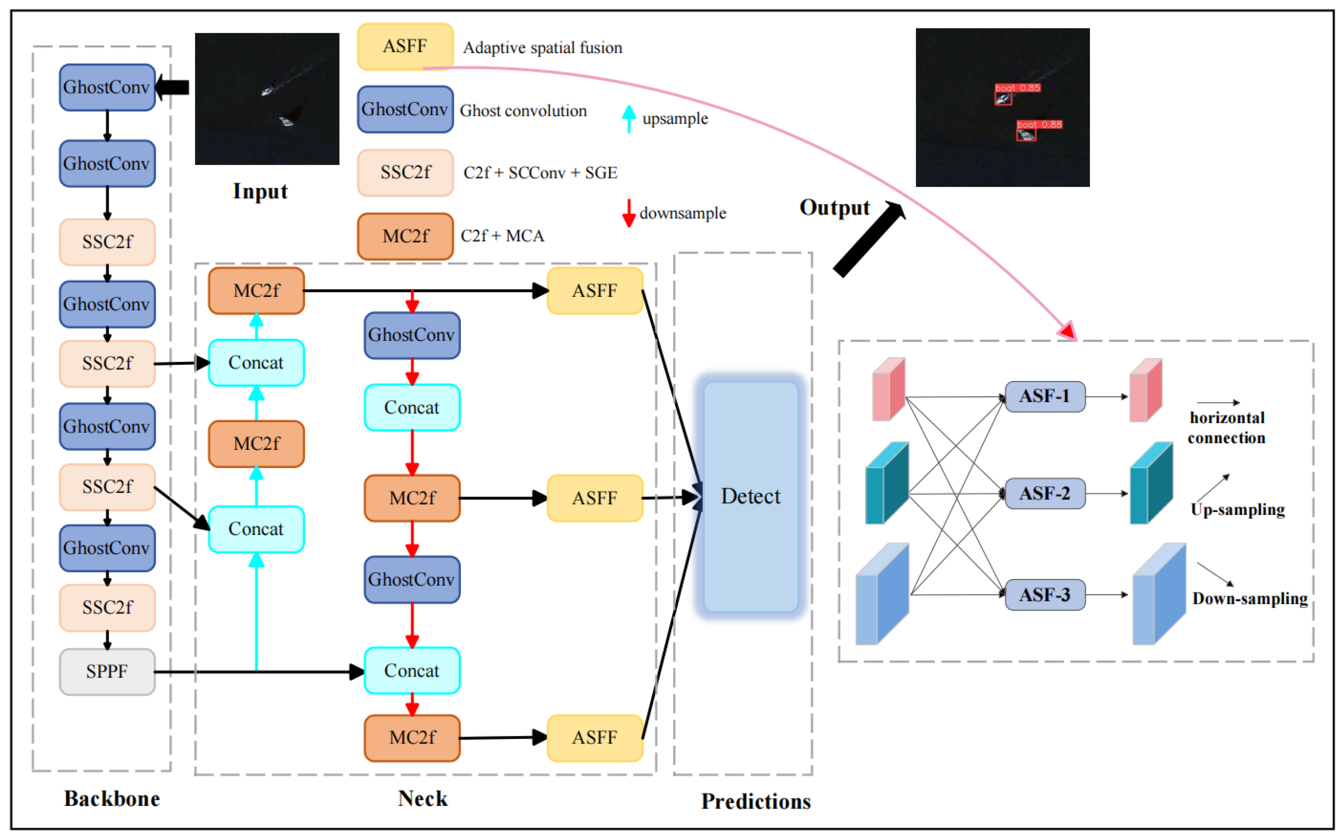
Figure 1. SSMA-YOLO model architecture.
Drones 08 00145 g001
Figure 2. Ghostconv module details.
Drones 08 00145 g002
Figure 3. SSC2f module details.
Drones 08 00145 g003
Figure 4. SRU and CRU module details.
Drones 08 00145 g004
Figure 5. SGE attention mechanism algorithm processing.
Drones 08 00145 g005
Figure 6. MC2f module details.
Drones 08 00145 g006
Figure 7. AFPN module details.
Drones 08 00145 g007
Figure 8. (a) The coordinate distribution diagram of the center point. (b) The width and height distribution diagram of the boundary box.
Drones 08 00145 g008
Figure 9. Target heatmaps obtained by Grad-CAM for YOLOv8n and SSMA-YOLO. (I) Original images from the Ships dataset. (II) Target heatmaps generated by YOLOv8n on the Ships dataset. (III) Target heatmaps generated by SSMA-YOLO on the Ships dataset.
Drones 08 00145 g009
Figure 10. P–R curves of YOLOv8n (black) and SSMA-YOLO (red).
Drones 08 00145 g010
Figure 11. Partial comparison target detection results of the Ships dataset, where (a,c,e,g) is the detection result of YOLOv8n and (b,d,f,h) is the detection result of SSMA-YOLO.
Drones 08 00145 g011
Table 1. Comparison results with the baseline model YOLOv8n.
ModelPrecision (%)Recall (%)F1 (%)mAP (%)Parameters (M)
YOLOv8n88.474.680.982.23.0
SSMA-YOLO91.679.485.186.62.3
Table 2. Ablation experiment results.
ModelmAP (%)Recall (%)F1(%)Precision (%)FLOPs (G)
YOLOv8n82.274.680.988.48.1
YOLOv8n + S 181.373.980.087.26.8
YOLOv8n + S + M 284.578.283.489.36.8
YOLOv8n + S + M + A 386.679.485.191.66.8
1 S means SSC2f module; 2 M means MC2f module; 3 A means AFPN module.
Table 3. Comparison of SSMA-YOLO with other models.
ModelPrecision (%)Recall (%)F1 (%)mAP (%)
Faster-RCNN80.870.175.177.4
SSD82.972.674.478.2
YOLOv383.773.478.279.6
YOLOv585.473.779.180.7
YOLOv787.674.280.381.8
SSMA-YOLO 91.679.485.186.6
Table 4. Comparison results on other datasets.
DatasetModelPrecision (%)Recall (%)F1 (%)mAP (%)
HRSC-2016Faster-RCNN84.381.482.884.5
SSD86.183.284.687.8
YOLOv387.384.485.889.1
YOLOv588.485.787.090.7
YOLOv790.686.288.391.8
YOLOv8n93.190.391.795.9
SSMA-YOLO95.795.495.597.3
SSDDFaster-RCNN83.980.282.079.9
SSD84.582.183.380.6
YOLOv385.283.484.382.2
YOLOv586.884.285.583.4
YOLOv788.685.687.184.8
YOLOv8n91.387.389.386.9
SSMA-YOLO 93.289.291.289.7
Disclaimer/Publisher’s Note: The statements, opinions and data contained in all publications are solely those of the individual author(s) and contributor(s) and not of MDPI and/or the editor(s). MDPI and/or the editor(s) disclaim responsibility for any injury to people or property resulting from any ideas, methods, instructions or products referred to in the content.