

A Study on Anti-Jamming Algorithms in Low-Earth-Orbit Satellite Signal-of-Opportunity Positioning Systems for Unmanned Aerial Vehicles

 ,
,
Abstract
1. Introduction
2. The Consecutive Mean Excision Based on Signal Cancellation (SCCME) Algorithm [35]
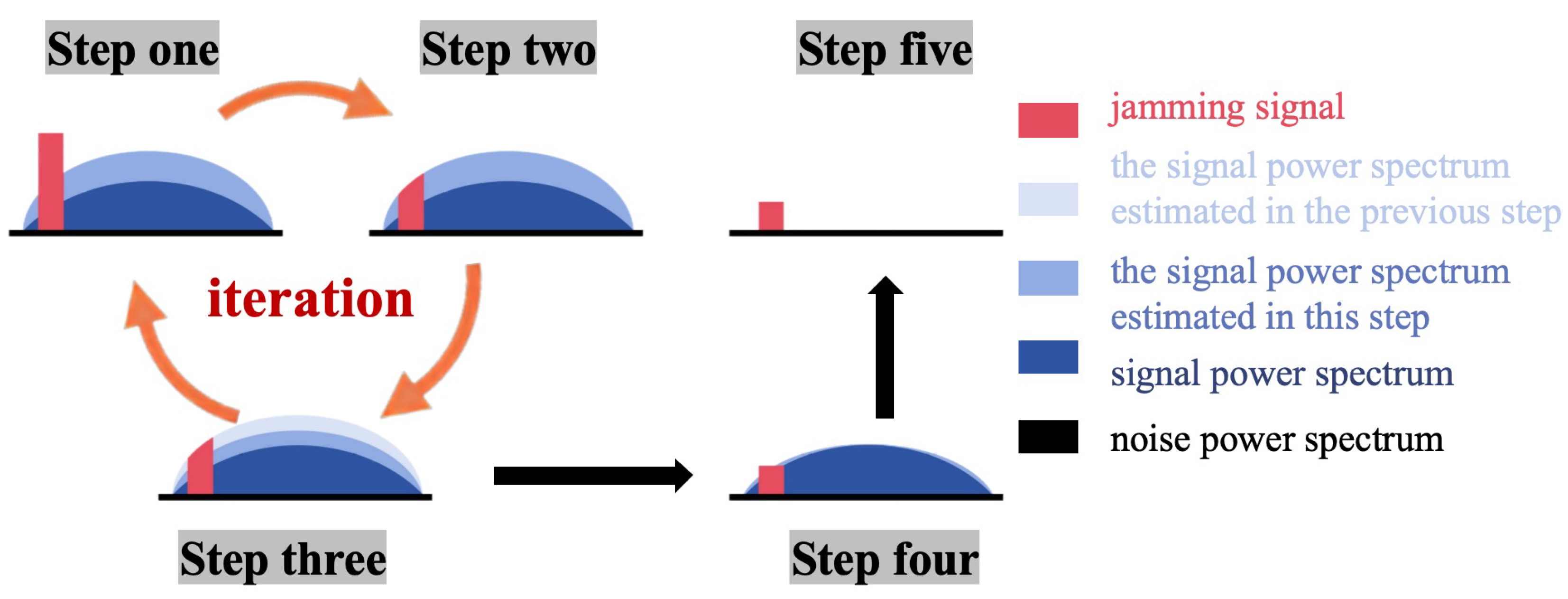
3. The Consecutive Iteration Based on Signal Cancellation (SCCI) Algorithm
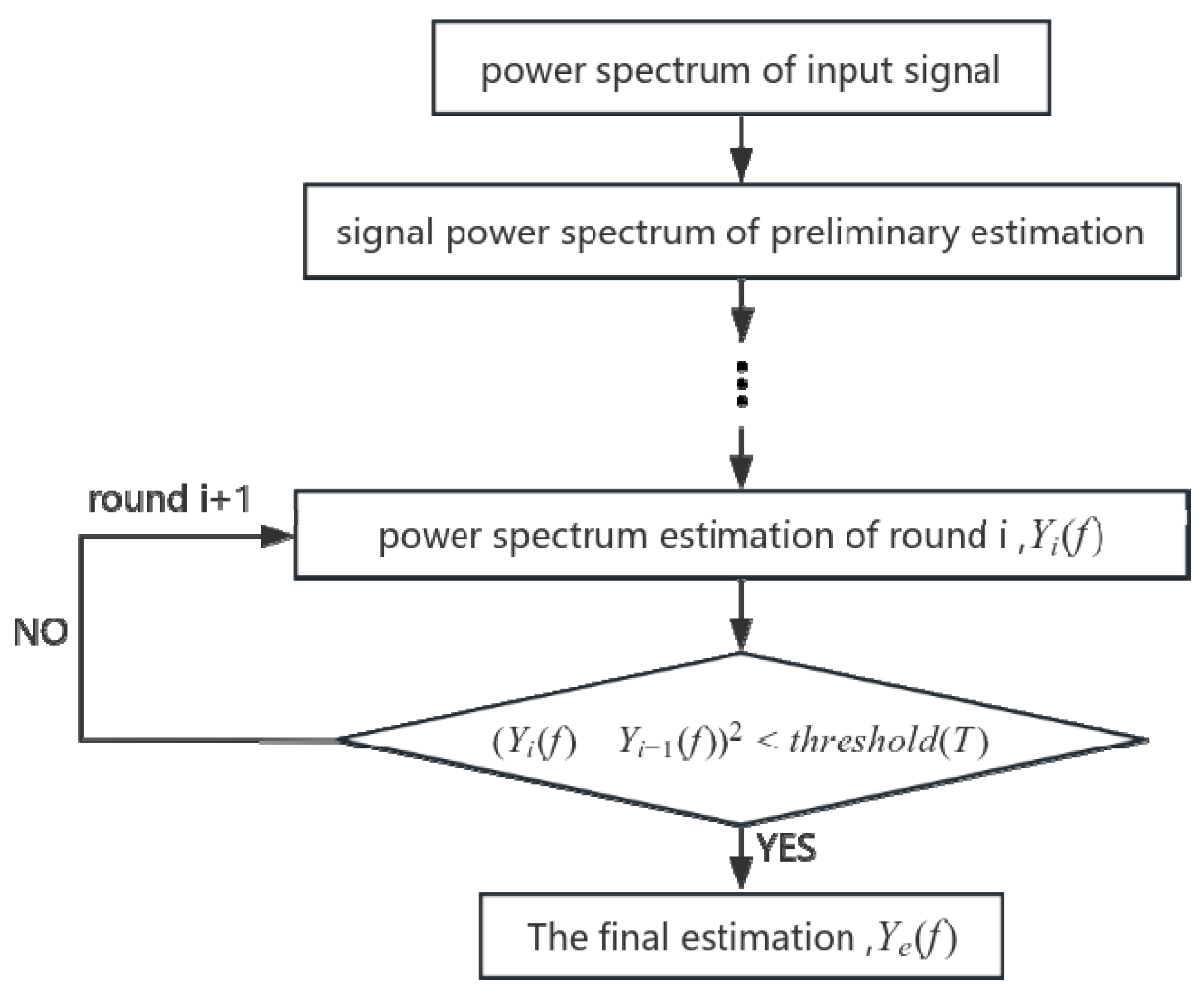
3.1. Process Optimization
3.2. Adaptive Variable Convergence Factor
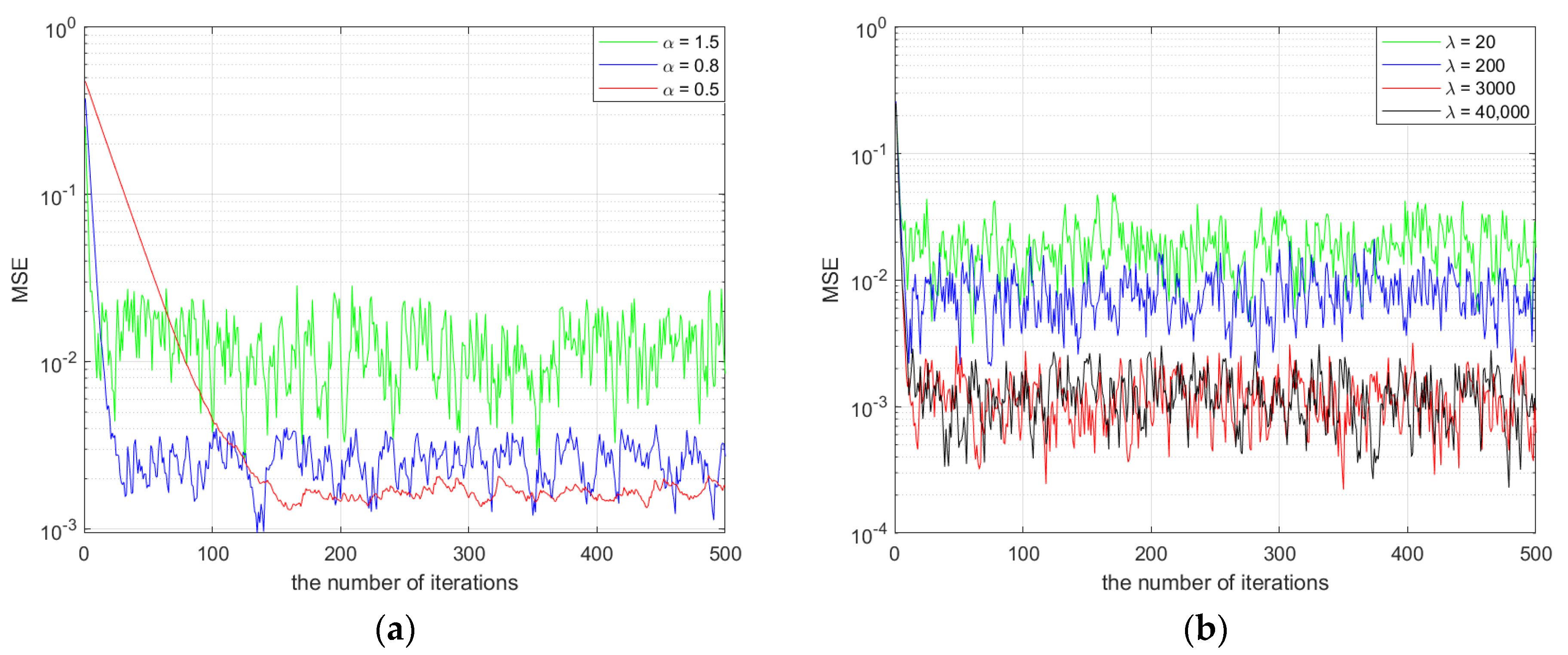
3.2.1. Parameter Settings
3.2.2. Analysis of the Parameters’ Impact on Performance
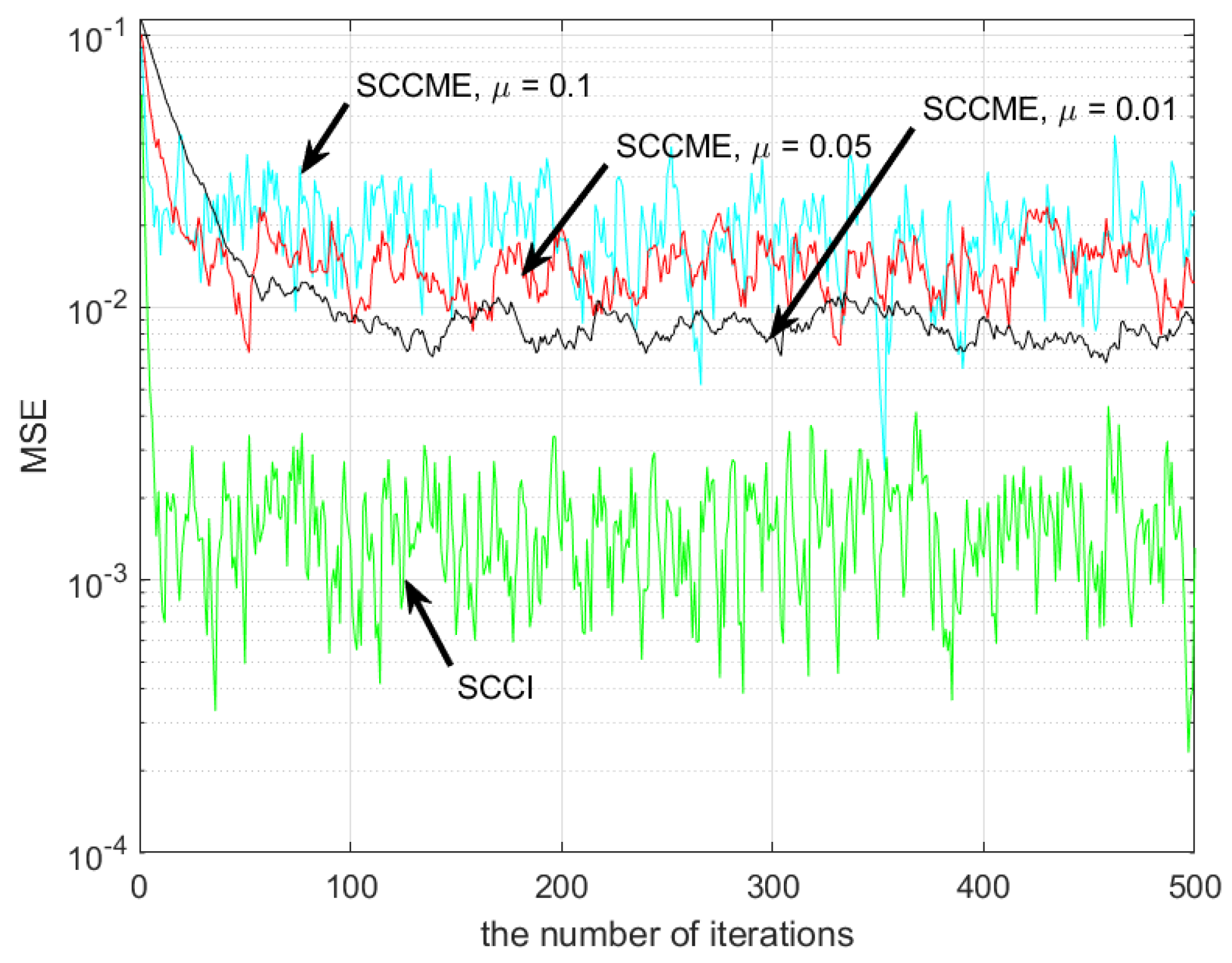
3.2.3. Performance Comparison of Algorithms
4. Simulation and Test Verification
4.1. Simulated Test
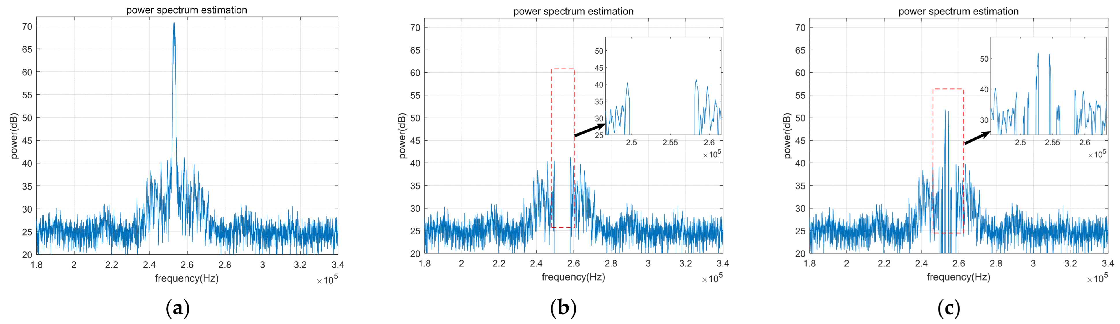
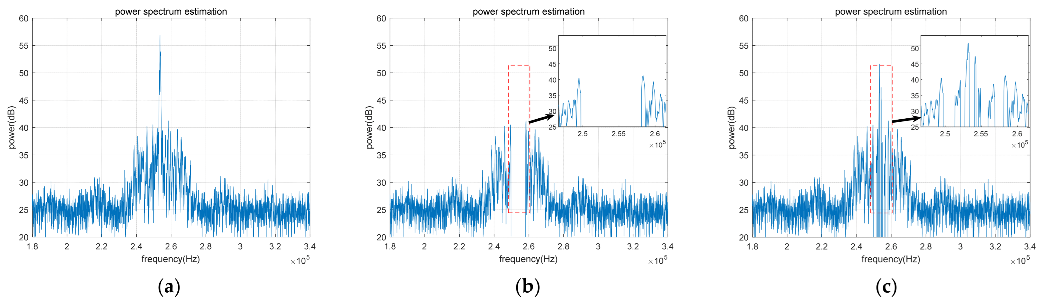
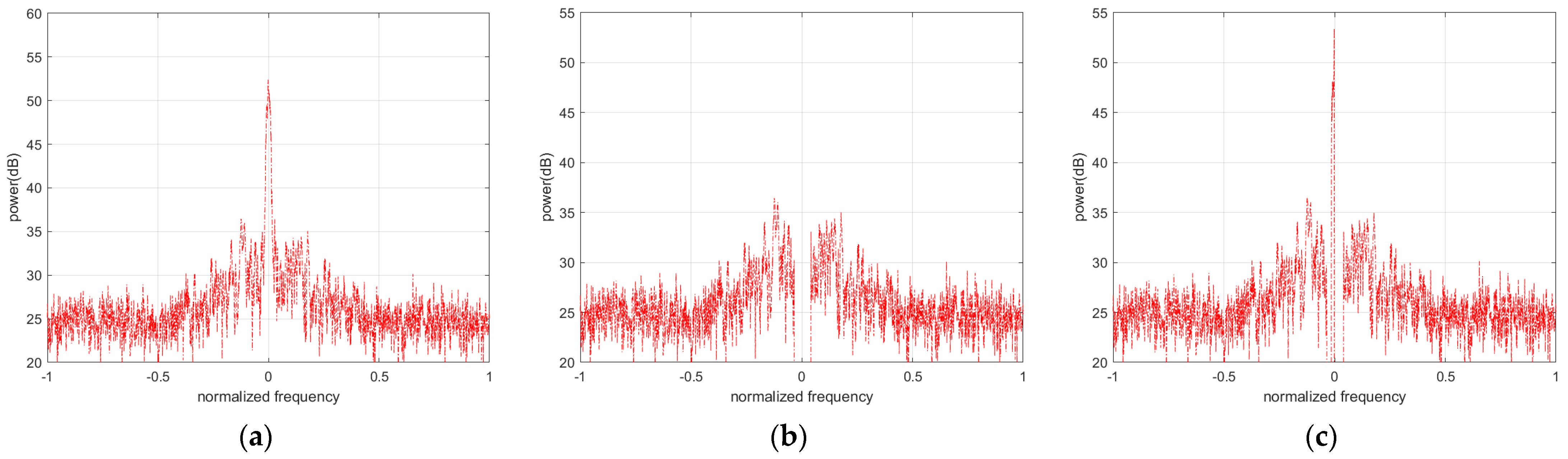
4.1.1. Signal Power Spectrum Simulation before and after Anti-Jamming
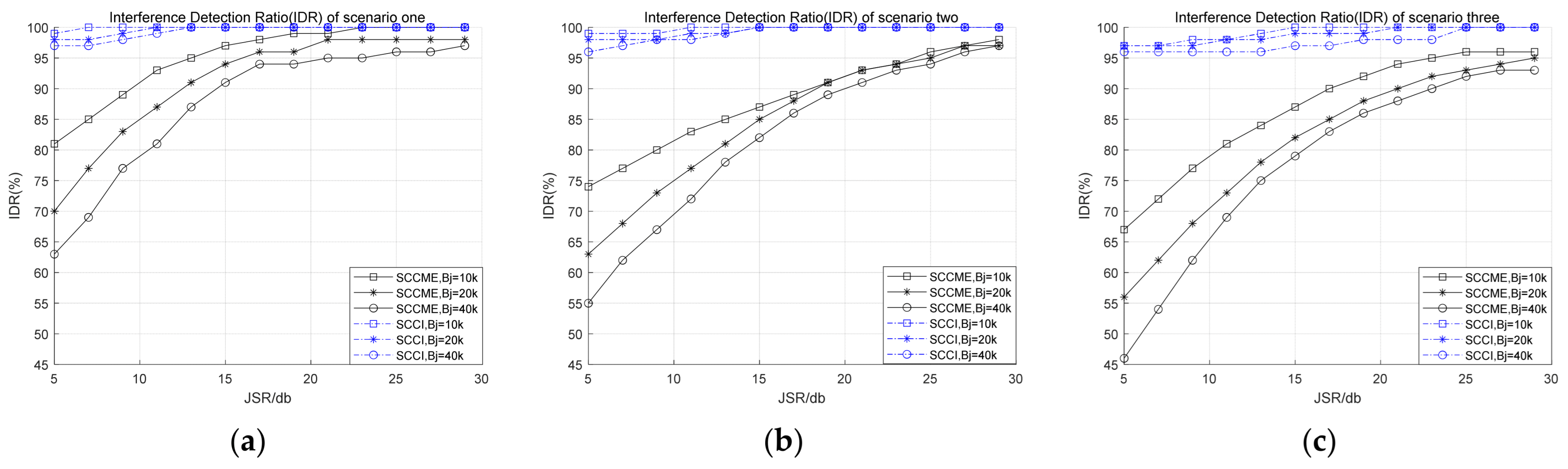
4.1.2. Simulation of Interference Detection Performance for Anti-Jamming Algorithm
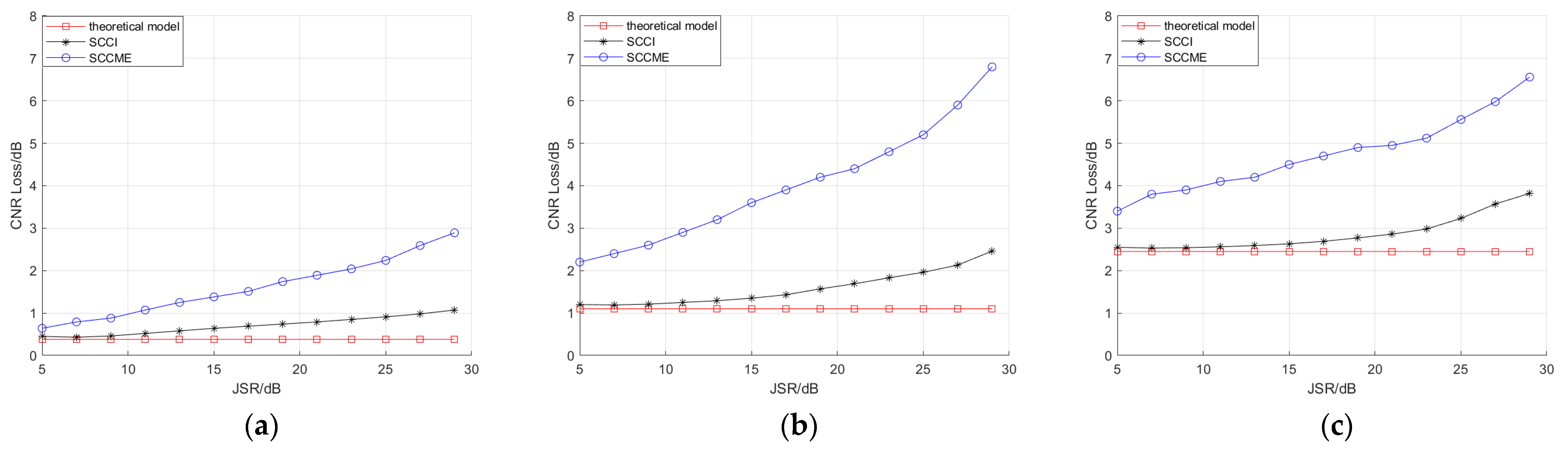
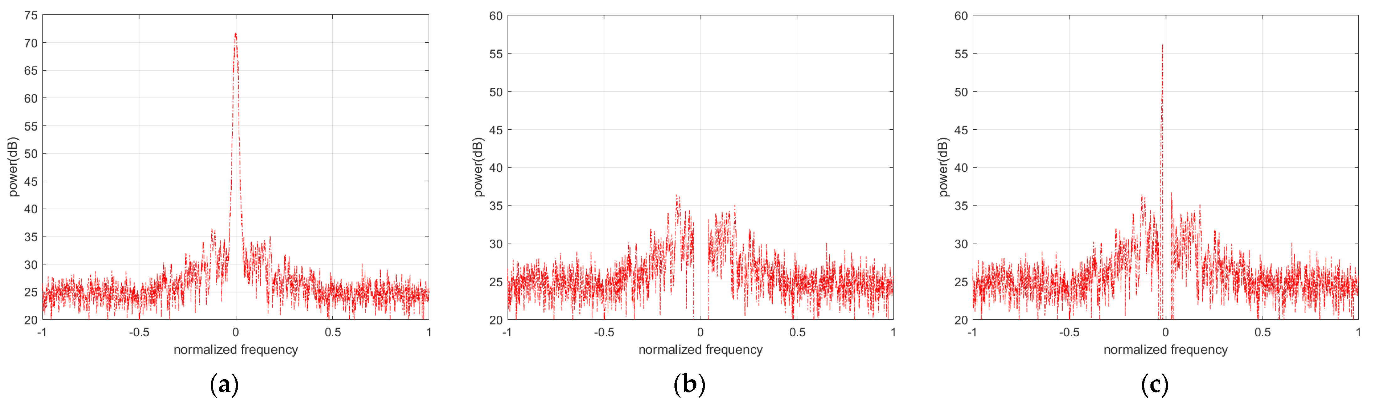
4.1.3. Verification of Anti-Jamming Performance
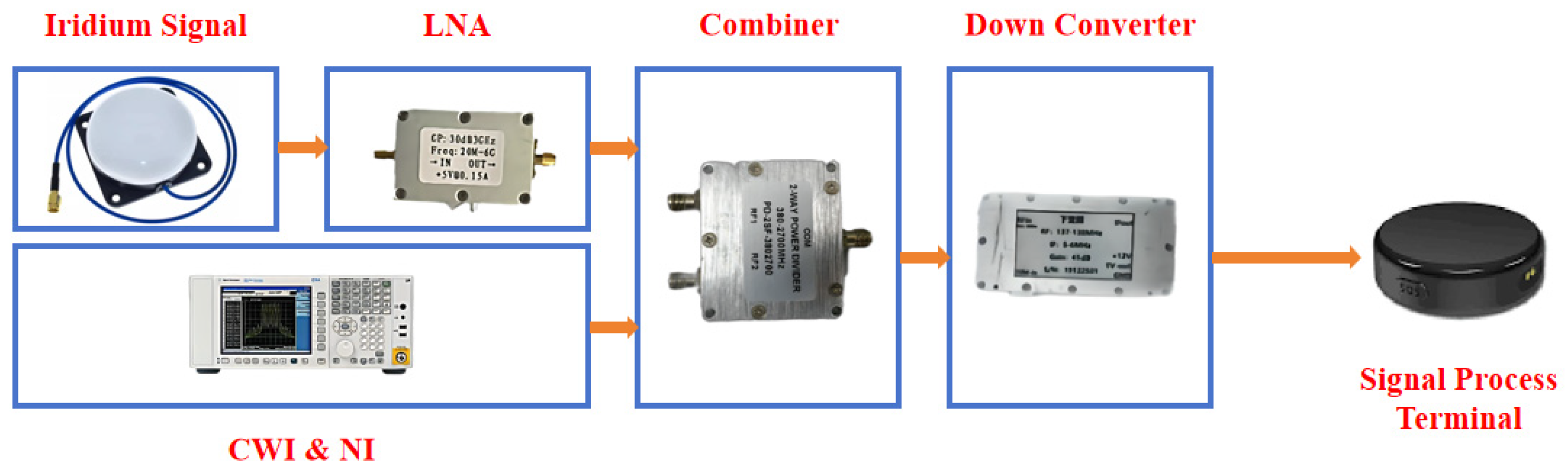
4.2. Actual Experimental Verification
5. Discussion
- (1)
- Using synthetic aperture technology, the moving UAV’s single antenna is combined with the UAV’s motion equation or the formation motion equation of multiple UAVs (which can be regarded as a one-dimensional array) to generate new spatial information. This synthesizes a single-point single antenna into a virtual antenna array, forming a pseudo-spatial anti-jamming technology that can effectively suppress complex interference situations caused by broadband or multiple jamming sources.
- (2)
- Establishing a background jamming signal type database and combining artificial intelligence for automatic detection and recognition, reconstructing jamming signals in the background, and then canceling them with the received signals to suppress interference can effectively suppress complex interference or multiple jamming sources. In ideal conditions, this can even achieve zero loss of useful signals.
6. Conclusions
Author Contributions
Funding
Data Availability Statement
Conflicts of Interest
References
- Liu, J.; Gao, K.; Guo, W.; Cui, J.; Guo, C. Role, path, and vision of “5G + BDS/GNSS”. Satell. Navig. 2020, 1, 23. [Google Scholar] [CrossRef]
- Psiaki, M.; Humphreys, T. Civilian GNSS Spoofing, Detection, and Recovery. In Position, Navigation, and Timing Technologies in the 21st Century; Morton, Y.T.J., Diggelen, F., Spilker, J.J., Parkinson, B.W., Lo, S., Gao, G., Eds.; Wiley Online Library: Hoboken, NJ, USA, 2020. [Google Scholar]
- LaST, DaviD. GNSS: The Present Imperfect. Inside GNSS 5.3. 2010; pp. 60–64. Available online: https://insidegnss-com.exactdn.com/wp-content/uploads/2018/01/may10-Last.pdf (accessed on 2 April 2024).
- Zidan, J.; Adegoke, E.I.; Kampert, E.; Birrell, S.A.; Ford, C.R.; Higgins, M.D. GNSS Vulnerabilities and Existing Solutions: A Review of the Literature. IEEE Access 2021, 9, 153960–153976. [Google Scholar] [CrossRef]
- Broumandan, A.; Jafarnia-Jahromi, A.; Daneshmand, S.; Lachapelle, G. Overview of Spatial Processing Approaches for GNSS Structural Interference Detection and Mitigation. Proc. IEEE 2016, 104, 1246–1257. [Google Scholar] [CrossRef]
- Salvatori, P.; Stallo, C.; Coluccia, A.; Neri, A.; Rispoli, F. An Integrity Monitoring Algorithm Design Based on Code Double Differences for Rail GNSS Augmentation Network. In Proceedings of the 2018 IEEE 4th International Forum on Research and Technology for Society and Industry (RTSI), Palermo, Italy, 10–13 September 2018; pp. 1–5. [Google Scholar]
- Kassas, Z.M.; Khalife, J.; Abdallah, A.A.; Lee, C. I Am Not Afraid of the GPS Jammer: Resilient Navigation Via Signals of Opportunity in GPS-Denied Environments. IEEE Aerosp. Electron. Syst. Mag. 2022, 37, 4–19. [Google Scholar] [CrossRef]
- Zhang, Y.; Ho, K.C. Localization by Signals of Opportunity in the Absence of Transmitter Position. IEEE Trans. Signal Process. 2022, 70, 4602–4617. [Google Scholar] [CrossRef]
- Hu, Z.; Li, S.; Xiang, Y. Time Information Transmission Based on FM Broadcast Signal. IEEE Access 2021, 9, 16360–16364. [Google Scholar] [CrossRef]
- Chen, L.; Yang, L.-L.; Chen, R. Time delay tracking for positioning in DTV networks. In Proceedings of the 2012 Ubiquitous Positioning, Indoor Navigation, and Location Based Service (UPINLBS), Helsinki, Finland, 3–4 October 2012; pp. 1–4. [Google Scholar]
- Han, K.; Yu, S.M.; Kim, S.-L.; Ko, S.-W. Exploiting User Mobility for WiFi RTT Positioning: A Geometric Approach. IEEE Internet Things J. 2021, 8, 14589–14606. [Google Scholar] [CrossRef]
- Neinavaie, M.; Khalife, J.; Kassas, Z.M. Cognitive Opportunistic Navigation in Private Networks With 5G Signals and Beyond. IEEE J. Sel. Top. Signal Process. 2022, 16, 129–143. [Google Scholar] [CrossRef]
- Zhao, C.; Qin, H.; Li, Z. Doppler Measurements From Multiconstellations in Opportunistic Navigation. IEEE Trans. Instrum. Meas. 2022, 71, 8500709. [Google Scholar] [CrossRef]
- Zhao, C.; Qin, H.; Wu, N.; Wang, D. Analysis of Baseline Impact on Differential Doppler Positioning and Performance Improvement Method for LEO Opportunistic Navigation. IEEE Trans. Instrum. Meas. 2023, 72, 1–10; [Google Scholar] [CrossRef]
- Duran, M.A.C.; D‘Amico, A.A.; Dardari, D.; Rydström, M.; Sottile, F.; Ström, E.G.; Taponecco, L. Chapter 3—Terrestrial Network-Based Positioning and Navigation. In Satellite and Terrestrial Radio Positioning Techniques; Dardari, D., Falletti, E., Luise, M., Eds.; Academic Press: Oxford, UK, 2012; pp. 75–153. [Google Scholar]
- Tan, Z.; Qin, H.; Cong, L.; Zhao, C. New Method for Positioning Using IRIDIUM Satellite Signals of Opportunity. IEEE Access 2019, 7, 83412–83423. [Google Scholar] [CrossRef]
- Neinavaie, M.; Khalife, J.; Kassas, Z.M. Acquisition, Doppler Tracking, and Positioning With Starlink LEO Satellites: First Results. IEEE Trans. Aerosp. Electron. Syst. 2022, 58, 2606–2610. [Google Scholar] [CrossRef]
- Morales, J.; Khalife, J.; Kassas, Z.M. Simultaneous Tracking of Orbcomm LEO Satellites and Inertial Navigation System Aiding Using Doppler Measurements. In Proceedings of the 2019 IEEE 89th Vehicular Technology Conference (VTC2019-Spring), Kuala Lumpur, Malaysia, 28 April–1 May 2019; pp. 1–6. [Google Scholar]
- Khairallah, N.; Kassas, Z.M. Ephemeris Closed-Loop Tracking of LEO Satellites with Pseudorange and Doppler Measurements. In Proceedings of the 34th International Technical Meeting of the Satellite Division of The Institute of Navigation (ION GNSS+ 2021), St. Louis, MO, USA, 20–24 September 2021; pp. 2544–2555. [Google Scholar]
- Morales-Ferre, R.; Lohan, E.S.; Falco, G.; Falletti, E. GDOP-based analysis of suitability of LEO constellations for future satellite-based positioning. In Proceedings of the 2020 IEEE International Conference on Wireless for Space and Extreme Environments (WiSEE), Vicenza, Italy, 12–14 October 2020; pp. 147–152. [Google Scholar]
- Leng, M.; Razul, S.G.; See, C.M.S.; Tay, W.P.; Cheng, C.; Quitin, F. Joint Navigation and Synchronization Using SOOP in GPS-Denied Environments: Algorithm and Empirical Study. In Proceedings of the 2015 Sensor Signal Processing for Defence (SSPD), Edinburgh, UK, 9–10 September 2015; IEEE: New York, NY, USA, 2015; pp. 1–5. [Google Scholar]
- Parkinson, B.W.; Spliker, J.J. Global Positioning System: Theory and Application; American Insitute of Aeronautics and Astronautics Inc.: Cambrige, MA, USA, 1996. [Google Scholar]
- Qin, H.; Zhang, Y. Positioning technology based on starlink signal of opportunity. J. Navig. Position. 2023, 11, 67–73. [Google Scholar]
- Jiang, Y.; Fu, J.; Li, B.; Jiang, P. Distributed Sensitivity and Critical Interference Power Analysis of Multi-Degree-of-Freedom Navigation Interference for Global Navigation Satellite System Array Antennas. Sensors 2024, 24, 650. [Google Scholar] [CrossRef] [PubMed]
- Cheng, J.; Ren, P.; Deng, T. A Novel Ranging and IMU-Based Method for Relative Positioning of Two-MAV Formation in GNSS-Denied Environments. Sensors 2023, 23, 4366. [Google Scholar] [CrossRef] [PubMed]
- Sun, Y.; Chen, F.; Lu, Z.; Wang, F. Anti-Jamming Method and Implementation for GNSS Receiver Based on Array Antenna Rotation. Remote Sens. 2022, 14, 4774. [Google Scholar] [CrossRef]
- Dong, P.; Cheng, J.; Liu, L. A Novel Anti-Jamming Technique for INS/GNSS Integration Based on Black Box Variational Inference. Appl. Sci. 2021, 11, 3664. [Google Scholar] [CrossRef]
- Shao, Y.; Ma, H.; Zhou, S.; Wang, X.; Antoniou, M.; Liu, H. Target Localization Based on Bistatic T/R Pair Selection in GNSS-Based Multistatic Radar System. Remote Sens. 2021, 13, 707. [Google Scholar] [CrossRef]
- Lemieszewski, Ł.; Radomska-Zalas, A.; Perec, A.; Dobryakova, L.; Ochin, E. GNSS and LNSS Positioning of Unmanned Transport Systems: The Brief Classification of Terrorist Attacks on USVs and UUVs. Electronics 2021, 10, 401. [Google Scholar] [CrossRef]
- Lu, Z.; Chen, F.; Xie, Y. High Precision Pseudo-Range Measurement in GNSS Anti-Jamming Antenna Array Processing. Electronics 2020, 9, 412. [Google Scholar] [CrossRef]
- Zhang, J.; Cui, X.; Xu, H.; Lu, M. A Two-Stage Interference Suppression Scheme Based on Antenna Array for GNSS Jamming and Spoofing. Sensors 2019, 19, 3870. [Google Scholar] [CrossRef] [PubMed]
- Wang, H.; Chang, Q.; Xu, Y. An Anti-Jamming Null-Steering Control Technique Based on Double Projection in Dynamic Scenes for GNSS Receivers. Sensors 2019, 19, 1661. [Google Scholar] [CrossRef] [PubMed]
- Xu, H.; Cui, X.; Lu, M. An SDR-Based Real-Time Testbed for GNSS Adaptive Array Anti-Jamming Algorithms Accelerated by GPU. Sensors 2016, 16, 356. [Google Scholar] [CrossRef] [PubMed]
- Nie, J. Study on GNSS Antenna Arrays Anti-Jamming Algorithm and Performance Evaluation Key Techniques. Ph.D. Thesis, National University of Defense Technology, Changsha, China, 2012. [Google Scholar]
- Li, J. Strong Interference Supression for Satellite Navigation Receiver with Single Antenna. Ph.D. Thesis, National University of Defense Technology, Changsha, China, 2016. [Google Scholar]
- O’brien, A.J. Adaptive Antenna Arrays for Precision GNSS Receivers; The Ohio State University: Columbus, OH, USA, 2009. [Google Scholar]
- Xie, Y.; Chen, F.; Huang, L.; Liu, Z.; Wang, F. Carrier phase biascorrelation for GNSS space-time array processing using time-delay data. GPS Solut. 2023, 27, 113. [Google Scholar] [CrossRef]
- Lu, Z. Research on Key Technology of Anti-jamming of Satellite Navigation Antenna Arrays. Ph.D. Thesis, National University of Defense Technology, Changsha, China, 2018. [Google Scholar]
- Lu, Z.; Chen, F.; Sun, Y.; Liu, Z.; Huang, L. Influence analysis of navigation signal power enhancement on array receiver. Syst. Eng. Electron. 2021, 43, 2581. [Google Scholar]
- Lu, Z.; Huang, L.; Nie, J.; Huang, Y.; Ou, G. Blind Anti-jamming Algorithm for Enhanced Signal Using Antenna Array. In Proceedings of the 8th China Satellite Navigation Conference (CSNC 2017), Shanghai, China, 23–25 May 2017; p. 5. [Google Scholar]
- Braun, T.M. Satellite Communications Payload and System; John Wiley & Sons: Hoboken, NJ, USA, 2012; pp. 552–559. [Google Scholar]
- Iridium Burst Detector and Demodulator. 2019. GNU Radio Iridium Out of Tree Module. Available online: https://github.com/muccc/gr-iridium (accessed on 4 July 2023).
- Iridium NEXT Engineering Statement. FCC File Number 1031348. Available online: https://fcc.report/IBFS/SAT-MOD-20131227-00148/1031348.pdf (accessed on 2 April 2024).
- Zhang, T.; Zhang, X.; Lu, M. Effect of frequency domain anti-jamming filter on satellite navigation signal tracking performance. In Proceedings of the China Satellite Navigation Conference (CSNC) 2013, Wuhan, China, 15–17 May 2013; pp. 507–516. [Google Scholar]


| SCCI Algorithm Specific Steps |
|---|
| Step 1: Obtain the power spectrum of the input signal, construct the power spectrum mean estimation model according to Equation (1), and update the model parameters following Equations (6) and (7). |
| Step 2: Extract the frequency points with power values higher than the estimated power spectrum, assign their values to the corresponding frequency points’ predicted power values for this iteration, and leave the power values of other frequency points unchanged to form a new set of signal power spectra. |
| Step 3: Repeat steps 1–2 iteratively until the iteration is complete, and then proceed to step 4. |
| Step 4: Subtract the estimated final iterative value from the true signal power spectrum. |
| Step 5: Obtain the power amplitude spectrum after removing the mean and initiate the threshold detection algorithm to identify the positions of interference spectral lines. |
| Parameters | Scene One | Scene Two | Scene Three |
|---|---|---|---|
| Jamming center frequency offset signal center frequency difference | 0 kHz | 100 kHz | 200 kHz |
| Jamming signal bandwidth | 10 kHz, 20 kHz, 40 kHz | ||
| JSR | 5 dB–30 dB, the step was 2 dB | ||
| Parameters | Scene One | Scene Two | Scene Three |
|---|---|---|---|
| Jamming signal bandwidth | 10 kHz | 20 kHz | 40 kHz |
| JSR | 5 dB–30 dB, the step was 2 dB | ||
Disclaimer/Publisher’s Note: The statements, opinions and data contained in all publications are solely those of the individual author(s) and contributor(s) and not of MDPI and/or the editor(s). MDPI and/or the editor(s) disclaim responsibility for any injury to people or property resulting from any ideas, methods, instructions or products referred to in the content. |
© 2024 by the authors. Licensee MDPI, Basel, Switzerland. This article is an open access article distributed under the terms and conditions of the Creative Commons Attribution (CC BY) license (https://creativecommons.org/licenses/by/4.0/).
Share and Cite
Yao, L.; Qin, H.; Gu, B.; Shi, G.; Sha, H.; Wang, M.; Xian, D.; Chen, F.; Lu, Z. A Study on Anti-Jamming Algorithms in Low-Earth-Orbit Satellite Signal-of-Opportunity Positioning Systems for Unmanned Aerial Vehicles. Drones 2024, 8, 164. https://doi.org/10.3390/drones8040164
Yao L, Qin H, Gu B, Shi G, Sha H, Wang M, Xian D, Chen F, Lu Z. A Study on Anti-Jamming Algorithms in Low-Earth-Orbit Satellite Signal-of-Opportunity Positioning Systems for Unmanned Aerial Vehicles. Drones. 2024; 8(4):164. https://doi.org/10.3390/drones8040164
Chicago/Turabian StyleYao, Lihao, Honglei Qin, Boyun Gu, Guangting Shi, Hai Sha, Mengli Wang, Deyong Xian, Feiqiang Chen, and Zukun Lu. 2024. "A Study on Anti-Jamming Algorithms in Low-Earth-Orbit Satellite Signal-of-Opportunity Positioning Systems for Unmanned Aerial Vehicles" Drones 8, no. 4: 164. https://doi.org/10.3390/drones8040164
APA StyleYao, L., Qin, H., Gu, B., Shi, G., Sha, H., Wang, M., Xian, D., Chen, F., & Lu, Z. (2024). A Study on Anti-Jamming Algorithms in Low-Earth-Orbit Satellite Signal-of-Opportunity Positioning Systems for Unmanned Aerial Vehicles. Drones, 8(4), 164. https://doi.org/10.3390/drones8040164