


Towards Fully Autonomous Drone Tracking by a Reinforcement Learning Agent Controlling a Pan–Tilt–Zoom Camera


Abstract
1. Introduction
1.1. Camera Configurations and Control Systems
- PTZ cameras: using a camera on a motorized pan–tilt platform. The FOR is greater than the FOV.
- Human camera control [13]: A human is controlling a camera to record a drone. This can be either a person filming a drone freehand or a human operator controlling a PTZ camera. The Anti-UAV dataset is an example of this, as it features videos of drones being followed by an operator. The FOR is larger than the FOV.
- Automated (integrated) PTZ camera control [14,15]: An automated control system for controlling the PTZ cameras to detect and track drones with no human operator. It relies on a drone detection mechanism and then a tracking mechanism for defining the control demands of the PTZ to keep the drone within the FOV. Some elements of this solution might be AI-based (e.g., the detection part).
- Detection: does the drone exist in the airspace volume of interest?
- Camera-based-tracking: if we detect the drone at time t, can we continuously move the pan–tilt–zoom camera to record the drone while it is in the airspace volume of interest?
- Classification: how do we know that the object being detected by the pan–tilt–zoom camera is a drone and not a bird?
1.2. Reinforcement Learning
1.3. Research Gap, Hypothesis, and Contribution
1.4. Layout
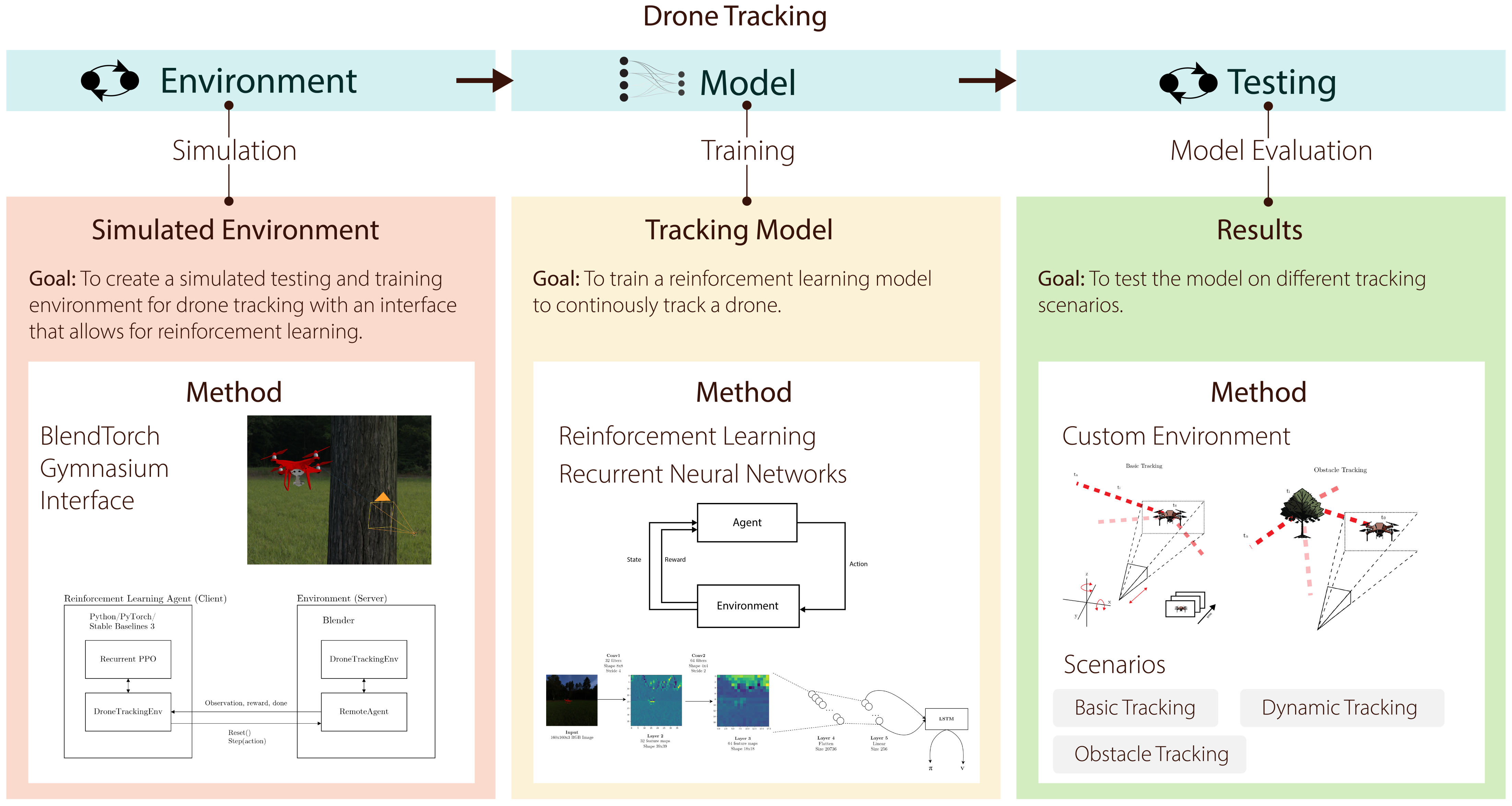
2. Methodology
2.1. Mathematical Description
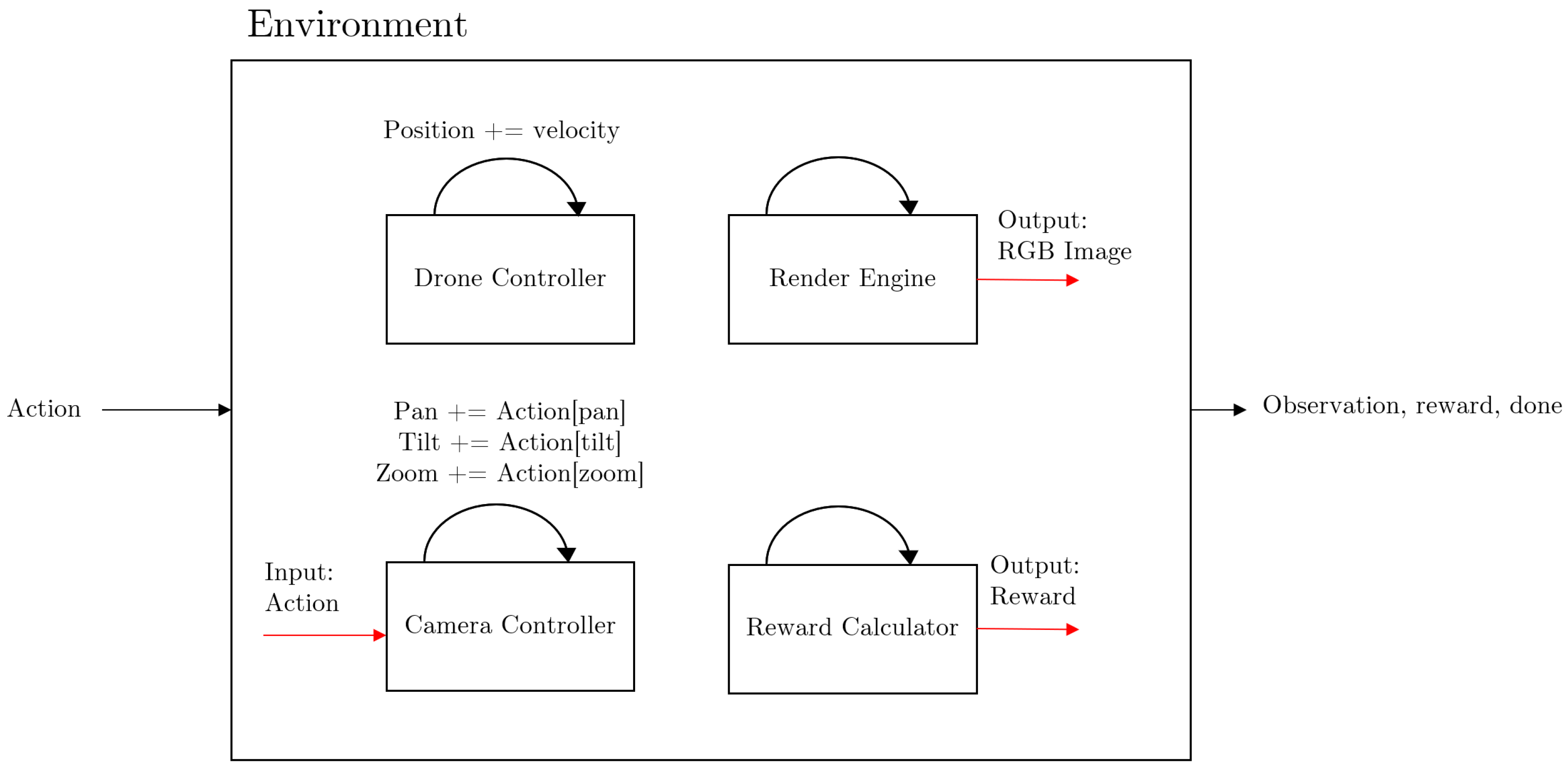
2.2. The Environment
2.2.1. Scenarios
- Basic Tracking. A random velocity is assigned at the beginning of each scenario. The drone follows this trajectory throughout.
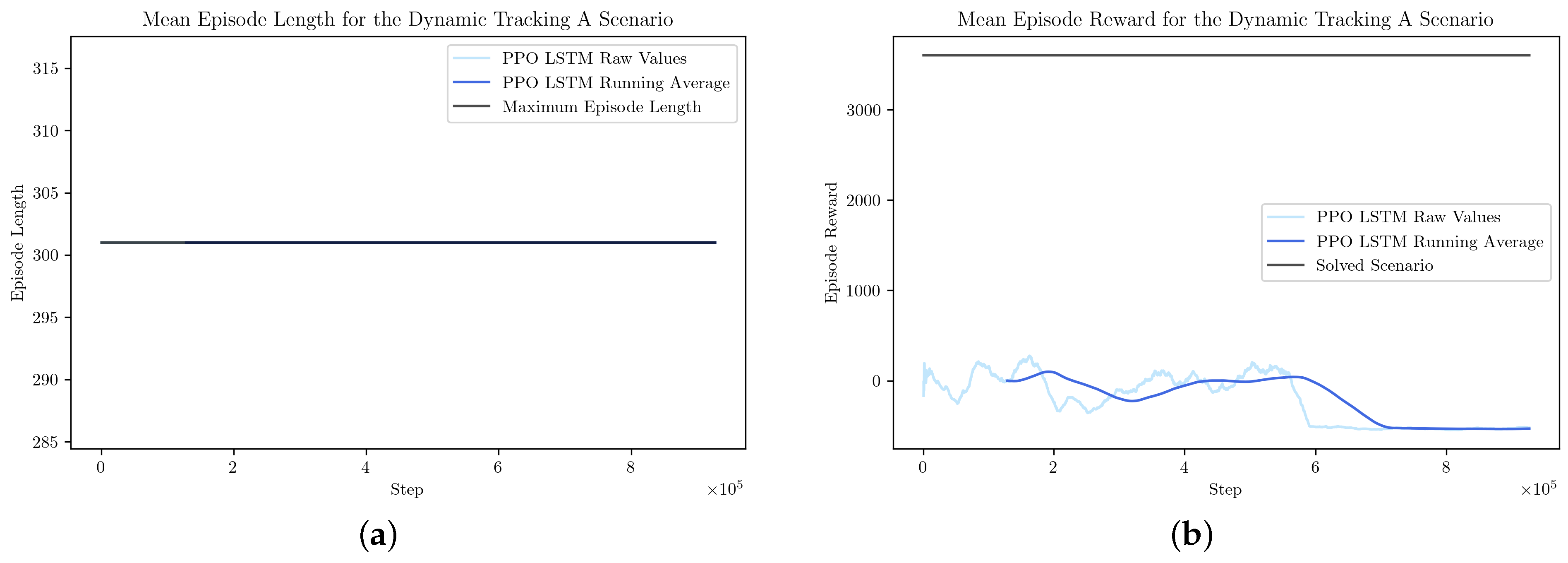
- Dynamic Tracking A. The movement of the drone is unpredictable. Every 30 steps (effectively, around 1 s) a new position target is assigned to the drone—hence changing the acceleration. Unlike in the basic tracking scenario where the trajectory is unchanging, we now have variable trajectories. The maximum drone velocity now exceeds that of the rotational velocity of the camera. Hence, it is possible for the drone to go completely out of bounds of the viewport, even when the requested rotational velocity is at its limit. Reward/termination mechanism is altered: termination only happens at 300 steps (and not when the drone is lost from the viewport). For every frame that a drone that is not visible in the viewport, −2 reward is accumulated. This allows the drone to disappear, and in principle, forces the agent to learn to re-detect the drone. This is a unique scenario in that it presents a challenge where the velocity of the drone might outpace that of the camera rotation. Human operators might be able to deal with this by understanding the expected path.
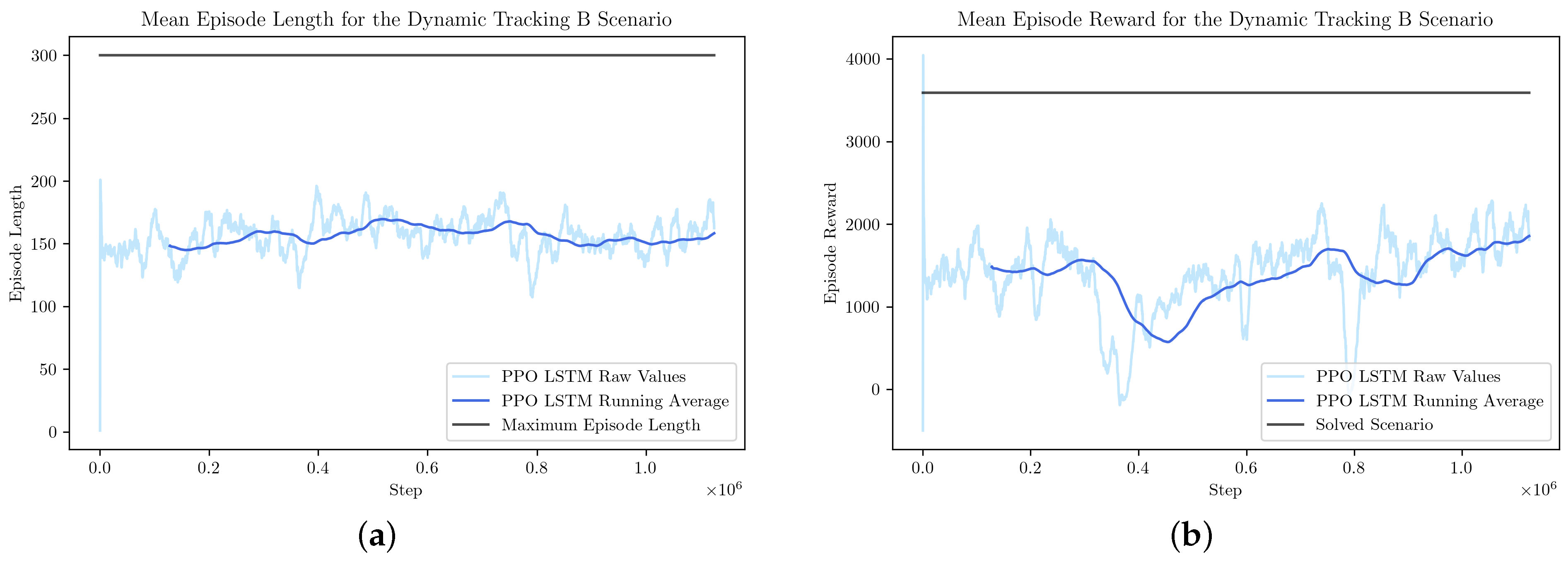
- Dynamic Tracking B. This is a variation of the Dynamic Tracking A scenario, with the dynamics of the drone tuned such that the maximum velocity should not outpace the maximum allowable rotational velocity of the camera. If the drone leaves the viewport, the agent is penalized (like in the Basic Tracking scenario).
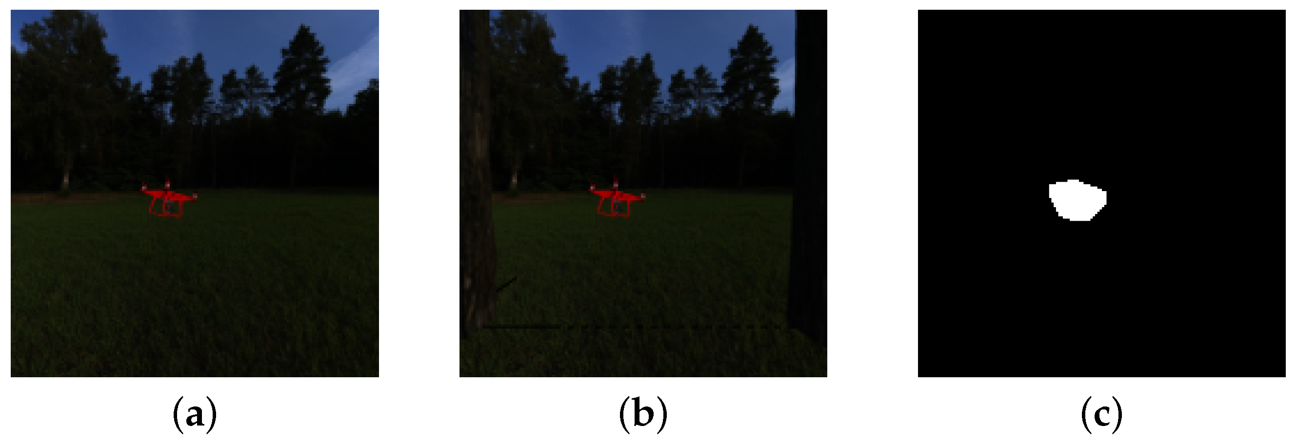
- Obstacle Tracking. The drone flies behind an obstacle. When behind the obstacle, the drone waits for a random amount of steps, between 0–100. After waiting, it flies to a randomly assigned position. This scenario was designed to challenge the tracker on whether it can deal with a context-dependent scenario—of anticipating a drone to reappear from behind an obstacle.

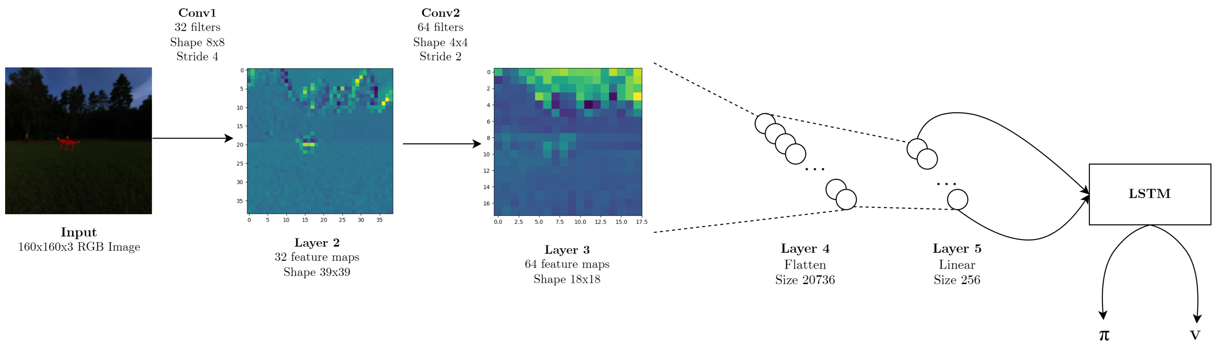
2.2.2. Observation
2.2.3. Action
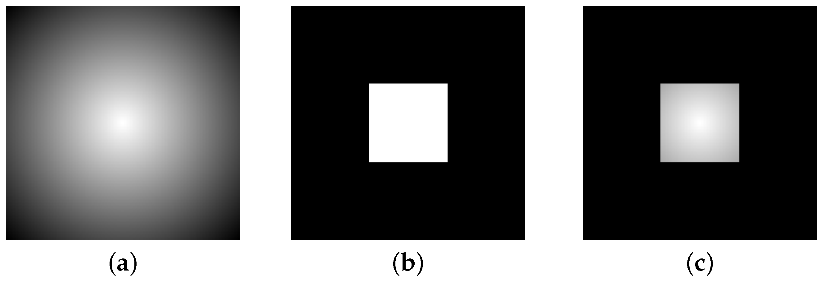
2.2.4. Reward and Termination
2.3. Reinforcement Learning Algorithms
3. Results
3.1. Basic Tracking
3.2. Dynamic Tracking A
3.3. Dynamic Tracking B
3.4. Obstacle Tracking
3.5. Discussion
4. Conclusions
5. Further Work
Author Contributions
Funding
Data Availability Statement
Conflicts of Interest
Abbreviations
| FOV | Field of View |
| FOR | Field of Regard |
| LSTM | Long Short-Term Memory |
| PTZ | Pan–Tilt–Zoom |
| RL | Reinforcement Learning |
| VOI | Volume of Interest |
References
- UK Counter-Unmanned Aircraft Strategy. p. 38. Available online: https://assets.publishing.service.gov.uk/media/5dad91d5ed915d42a3e43a13/Counter-Unmanned_Aircraft_Strategy_Web_Accessible.pdf (accessed on 20 May 2024).
- Wisniewski, M.; Rana, Z.A.; Petrunin, I. Reinforcement Learning for Pan-Tilt-Zoom Camera Control, with Focus on Drone Tracking. In Proceedings of the AIAA SCITECH 2023 Forum, National Harbor, MD, USA, Online, 23–27 January 2023. [Google Scholar] [CrossRef]
- UAS Airspace Restrictions Guidance and Policy 2022. Available online: https://www.caa.co.uk/publication/download/18207 (accessed on 5 April 2024).
- Jahangir, M.; Baker, C. Robust Detection of Micro-UAS Drones with L-Band 3-D Holographic Radar. In Proceedings of the 2016 Sensor Signal Processing for Defence (SSPD), Edinburgh, UK, 22–23 September 2016; pp. 1–5. [Google Scholar] [CrossRef]
- Doumard, T.; Riesco, F.G.; Petrunin, I.; Panagiotakopoulos, D.; Bennett, C.; Harman, S. Radar Discrimination of Small Airborne Targets Through Kinematic Features and Machine Learning. In Proceedings of the 2022 IEEE/AIAA 41st Digital Avionics Systems Conference (DASC), Portsmouth, VA, USA, 18–22 September 2022; pp. 1–10. [Google Scholar] [CrossRef]
- White, D.; Jahangir, M.; Wayman, J.P.; Reynolds, S.J.; Sadler, J.P.; Antoniou, M. Bird and Micro-Drone Doppler Spectral Width and Classification. In Proceedings of the 2023 24th International Radar Symposium (IRS), Berlin, Germany, 24–26 May 2023; pp. 1–10. [Google Scholar] [CrossRef]
- Seidaliyeva, U.; Akhmetov, D.; Ilipbayeva, L.; Matson, E.T. Real-Time and Accurate Drone Detection in a Video with a Static Background. Sensors 2020, 20, 3856. [Google Scholar] [CrossRef]
- Mueller, T.; Erdnuess, B. Robust Drone Detection with Static VIS and SWIR Cameras for Day and Night Counter-UAV. In Proceedings of the Counterterrorism, Crime Fighting, Forensics, and Surveillance Technologies III, Strasbourg, France, 9–12 September 2019; p. 10. [Google Scholar] [CrossRef]
- Coluccia, A.; Fascista, A.; Schumann, A.; Sommer, L.; Ghenescu, M.; Avenue, A.O.; Piatrik, T. Drone-vs-Bird Detection Challenge at IEEE AVSS2019. In Proceedings of the 16th IEEE International Conference on Advanced Video and Signal Based Surveillance, AVSS 2019, Taipei, Taiwan, 18–21 September 2019; p. 7. [Google Scholar]
- Demir, B.; Ergunay, S.; Nurlu, G.; Popovic, V.; Ott, B.; Wellig, P.; Thiran, J.P.; Leblebici, Y. Real-Time High-Resolution Omnidirectional Imaging Platform for Drone Detection and Tracking. J. Real-Time Image Process. 2020, 17, 1625–1635. [Google Scholar] [CrossRef]
- Liu, H.; Wei, Z.; Chen, Y.; Pan, J.; Lin, L.; Ren, Y. Drone Detection Based on an Audio-Assisted Camera Array. In Proceedings of the 2017 IEEE Third International Conference on Multimedia Big Data (BigMM), Laguna Hills, CA, USA, 19–21 April 2017; pp. 402–406. [Google Scholar] [CrossRef]
- Mediavilla, C.; Nans, L.; Marez, D.; Parameswaran, S. Detecting Aerial Objects: Drones, Birds, and Helicopters. In Proceedings of the Artificial Intelligence and Machine Learning in Defense Applications III, Online, Spain, 13–18 September 2021; p. 18. [Google Scholar] [CrossRef]
- Jiang, N.; Wang, K.; Peng, X.; Yu, X.; Wang, Q.; Xing, J.; Li, G.; Zhao, J.; Guo, G.; Han, Z. Anti-UAV: A Large Multi-Modal Benchmark for UAV Tracking. arXiv 2021, arXiv:2101.08466. [Google Scholar]
- Liu, Y.; Liao, L.; Wu, H.; Qin, J.; He, L.; Yang, G.; Zhang, H.; Zhang, J. Trajectory and Image-Based Detection and Identification of UAV. Vis. Comput. 2020, 37, 1769–1780. [Google Scholar] [CrossRef]
- Svanstrom, F.; Englund, C.; Alonso-Fernandez, F. Real-Time Drone Detection and Tracking with Visible, Thermal and Acoustic Sensors. In Proceedings of the 25th International Conference on Pattern Recognition, ICPR 2020, Virtual Event, Milan, Italy, 10–15 January 2021. [Google Scholar]
- Sandha, S.S.; Balaji, B.; Garcia, L.; Srivastava, M. Eagle: End-to-end Deep Reinforcement Learning Based Autonomous Control of PTZ Cameras. In Proceedings of the 8th ACM/IEEE Conference on Internet of Things Design and Implementation, San Antonio, TX, USA, 9–12 May 2023; pp. 144–157. [Google Scholar] [CrossRef]
- Fahim, A.; Papalexakis, E.; Krishnamurthy, S.V.; Chowdhury, A.K.R.; Kaplan, L.; Abdelzaher, T. AcTrak: Controlling a Steerable Surveillance Camera Using Reinforcement Learning. ACM Trans. Cyber-Phys. Syst. 2023, 7, 1–27. [Google Scholar] [CrossRef]
- Isaac-Medina, B.K.S.; Poyser, M.; Organisciak, D.; Willcocks, C.G.; Breckon, T.P.; Shum, H.P.H. Unmanned Aerial Vehicle Visual Detection and Tracking Using Deep Neural Networks: A Performance Benchmark. In Proceedings of the 2021 IEEE/CVF International Conference on Computer Vision Workshops (ICCVW), Montreal, BC, Canada, 11–17 October 2021; pp. 1223–1232. [Google Scholar] [CrossRef]
- Meinhardt, T.; Kirillov, A.; Leal-Taixe, L.; Feichtenhofer, C. TrackFormer: Multi-Object Tracking with Transformers. In Proceedings of the IEEE/CVF Conference on Computer Vision and Pattern Recognition, CVPR 2022, New Orleans, LA, USA, 18–24 June 2022; p. 16. [Google Scholar]
- Bewley, A.; Ge, Z.; Ott, L.; Ramos, F.; Upcroft, B. Simple Online and Realtime Tracking. In Proceedings of the 2016 IEEE International Conference on Image Processing (ICIP), Phoenix, AZ, USA, 25–28 September 2016; pp. 3464–3468. [Google Scholar] [CrossRef]
- Li, B.; Wu, W.; Wang, Q.; Zhang, F.; Xing, J.; Yan, J. SiamRPN++: Evolution of Siamese Visual Tracking with Very Deep Networks. In Proceedings of the IEEE Conference on Computer Vision and Pattern Recognition, CVPR 2019, Long Beach, CA, USA, 16–20 June 2019. [Google Scholar]
- Scholes, S.; Ruget, A.; Mora-Martin, G.; Zhu, F.; Gyongy, I.; Leach, J. DroneSense: The Identification, Segmentation, and Orientation Detection of Drones via Neural Networks. IEEE Access 2022, 10, 38154–38164. [Google Scholar] [CrossRef]
- Wisniewski, M.; Rana, Z.A.; Petrunin, I. Drone Model Classification Using Convolutional Neural Network Trained on Synthetic Data. J. Imaging 2022, 8, 218. [Google Scholar] [CrossRef]
- Silver, D.; Huang, A.; Maddison, C.J.; Guez, A.; Sifre, L.; van den Driessche, G.; Schrittwieser, J.; Antonoglou, I.; Panneershelvam, V.; Lanctot, M.; et al. Mastering the game of Go with deep neural networks and tree search. Nature 2016, 529, 484–489. [Google Scholar] [CrossRef]
- Jumper, J.; Evans, R.; Pritzel, A.; Green, T.; Figurnov, M.; Ronneberger, O.; Tunyasuvunakool, K.; Bates, R.; Žídek, A.; Potapenko, A.; et al. Highly accurate protein structure prediction with AlphaFold. Nature 2021, 596, 583–589. [Google Scholar] [CrossRef]
- Berner, C.; Brockman, G.; Chan, B.; Cheung, V.; Dębiak, P.; Dennison, C.; Farhi, D.; Fischer, Q.; Hashme, S.; Hesse, C.; et al. Dota 2 with Large Scale Deep Reinforcement Learning. arXiv 2019, arXiv:1912.06680. [Google Scholar]
- Mnih, V.; Kavukcuoglu, K.; Silver, D.; Graves, A.; Antonoglou, I.; Wierstra, D.; Riedmiller, M. Playing Atari with Deep Reinforcement Learning. arXiv 2013, arXiv:1312.5602. [Google Scholar]
- Mnih, V.; Kavukcuoglu, K.; Silver, D.; Rusu, A.A.; Veness, J.; Bellemare, M.G.; Graves, A.; Riedmiller, M.; Fidjeland, A.K.; Ostrovski, G.; et al. Human-Level Control through Deep Reinforcement Learning. Nature 2015, 518, 529–533. [Google Scholar] [CrossRef]
- Chen, C.; Ying, V.; Laird, D. Deep Q-Learning with Recurrent Neural Networks. p. 6. Available online: https://cs229.stanford.edu/proj2016/report/ChenYingLaird-DeepQLearningWithRecurrentNeuralNetwords-report.pdf (accessed on 20 May 2024).
- Hausknecht, M.; Stone, P. Deep Recurrent Q-Learning for Partially Observable MDPs. arXiv 2017, arXiv:1507.06527. [Google Scholar]
- Qi, H.; Yi, B.; Suresh, S.; Lambeta, M.; Ma, Y.; Calandra, R.; Malik, J. General In-Hand Object Rotation with Vision and Touch. In Proceedings of the Conference on Robot Learning, CoRL 2023, Atlanta, GA, USA, 6–9 November 2023. [Google Scholar]
- Hafner, D.; Pasukonis, J.; Ba, J.; Lillicrap, T. Mastering Diverse Domains through World Models. arXiv 2023, arXiv:2301.04104. [Google Scholar]
- Kumar, A.; Fu, Z.; Pathak, D.; Malik, J. RMA: Rapid Motor Adaptation for Legged Robots. In Proceedings of the Robotics: Science and Systems XVII, Robotics: Science and Systems Foundation, Virtual Event, 12–16 July 2021. [Google Scholar] [CrossRef]
- Lample, G.; Chaplot, D.S. Playing FPS Games with Deep Reinforcement Learning. In Proceedings of the Thirty-First AAAI Conference on Artificial Intelligence, San Francisco, CA, USA, 4–9 February 2017. [Google Scholar]
- Kempka, M.; Wydmuch, M.; Runc, G.; Toczek, J.; Jaśkowski, W. ViZDoom: A Doom-based AI Research Platform for Visual Reinforcement Learning. In Proceedings of the 2016 IEEE Conference on Computational Intelligence and Games (CIG), Santorini, Greece, 20–23 September 2016. [Google Scholar]
- Brockman, G.; Cheung, V.; Pettersson, L.; Schneider, J.; Schulman, J.; Tang, J.; Zaremba, W. OpenAI Gym. arXiv 2016, arXiv:1606.01540. [Google Scholar]
- Mirowski, P.; Pascanu, R.; Viola, F.; Soyer, H.; Ballard, A.J.; Banino, A.; Denil, M.; Goroshin, R.; Sifre, L.; Kavukcuoglu, K.; et al. Learning to Navigate in Complex Environments. In Proceedings of the 5th International Conference on Learning Representations, ICLR 2017, Toulon, France, 24–26 April 2017. [Google Scholar]
- Sadeghi, F.; Levine, S. CAD2RL: Real Single-Image Flight without a Single Real Image. In Proceedings of the Robotics: Science and Systems XIII, Cambridge, MA, USA, 12–16 July 2017. [Google Scholar]
- Vorbach, C.; Hasani, R.; Amini, A.; Lechner, M.; Rus, D. Causal Navigation by Continuous-time Neural Networks. In Proceedings of the Advances in Neural Information Processing Systems 34: Annual Conference on Neural Information Processing Systems 2021, NeurIPS 2021, Virtual, 6–14 December 2021. [Google Scholar]
- Kaufmann, E.; Bauersfeld, L.; Loquercio, A.; Müller, M.; Koltun, V.; Scaramuzza, D. Champion-Level Drone Racing Using Deep Reinforcement Learning. Nature 2023, 620, 982–987. [Google Scholar] [CrossRef]
- Pham, H.X.; La, H.M.; Feil-Seifer, D.; Nefian, A. Cooperative and Distributed Reinforcement Learning of Drones for Field Coverage. arXiv 2018, arXiv:1803.07250. [Google Scholar]
- Muñoz, G.; Barrado, C.; Çetin, E.; Salami, E. Deep Reinforcement Learning for Drone Delivery. Drones 2019, 3, 72. [Google Scholar] [CrossRef]
- Akhloufi, M.A.; Arola, S.; Bonnet, A. Drones Chasing Drones: Reinforcement Learning and Deep Search Area Proposal. Drones 2019, 3, 58. [Google Scholar] [CrossRef]
- Morad, S.; Kortvelesy, R.; Bettini, M.; Liwicki, S.; Prorok, A. POPGym: Benchmarking Partially Observable Reinforcement Learning. arXiv 2023, arXiv:2303.01859. [Google Scholar]
- Heindl, C.; Brunner, L.; Zambal, S.; Scharinger, J. BlendTorch: A Real-Time, Adaptive Domain Randomization Library. In Proceedings of the Pattern Recognition, ICPR International Workshops and Challenges, Virtual Event, 10–15 January 2021. [Google Scholar]
- Heindl, C.; Zambal, S.; Scharinger, J. Learning to Predict Robot Keypoints Using Artificially Generated Images. In Proceedings of the 2019 24th IEEE International Conference on Emerging Technologies and Factory Automation (ETFA), Zaragoza, Spain, 10–13 September 2019. [Google Scholar]
- Towers, M.; Terry, J.K.; Kwiatkowski, A.; Balis, J.U.; Cola, G.D.; Deleu, T.; Goulão, M.; Kallinteris, A.; KG, A.; Krimmel, M.; et al. Gymnasium (v0.28.1). Zenodo. 2023. Available online: https://zenodo.org/records/8127026 (accessed on 20 May 2024).
- Raffin, A.; Hill, A.; Gleave, A.; Kanervisto, A.; Ernestus, M.; Dormann, N. Stable-Baselines3: Reliable Reinforcement Learning Implementations. J. Mach. Learn. Res. 2021, 22, 1–8. [Google Scholar]
- Paszke, A.; Gross, S.; Massa, F.; Lerer, A.; Bradbury, J.; Chanan, G.; Killeen, T.; Lin, Z.; Gimelshein, N.; Antiga, L.; et al. PyTorch: An Imperative Style, High-Performance Deep Learning Library. In Proceedings of the Advances in Neural Information Processing Systems 32: Annual Conference on Neural Information Processing Systems 2019, NeurIPS 2019, Vancouver, BC, Canada, 8–14 December 2019; p. 12. [Google Scholar]
- Schulman, J.; Wolski, F.; Dhariwal, P.; Radford, A.; Klimov, O. Proximal Policy Optimization Algorithms. arXiv 2017, arXiv:1707.06347. [Google Scholar]
- Kosmatopoulos, E.; Polycarpou, M.; Christodoulou, M.; Ioannou, P. High-Order Neural Network Structures for Identification of Dynamical Systems. IEEE Trans. Neural Netw. 1995, 6, 422–431. [Google Scholar] [CrossRef] [PubMed]
- Chow, T.; Fang, Y. A Recurrent Neural-Network-Based Real-Time Learning Control Strategy Applying to Nonlinear Systems with Unknown Dynamics. IEEE Trans. Ind. Electron. 1998, 45, 151–161. [Google Scholar] [CrossRef]
- Tobin, J.; Fong, R.; Ray, A.; Schneider, J.; Zaremba, W.; Abbeel, P. Domain Randomization for Transferring Deep Neural Networks from Simulation to the Real World. In Proceedings of the 2017 IEEE/RSJ International Conference on Intelligent Robots and Systems (IROS), Vancouver, BC, Canada, 24–28 September 2017; pp. 23–30. [Google Scholar] [CrossRef]
- Hasani, R.; Lechner, M.; Amini, A.; Rus, D.; Grosu, R. Liquid Time-constant Networks. arXiv 2020, arXiv:2006.04439. [Google Scholar] [CrossRef]
- Team, D.I.A.; Abramson, J.; Ahuja, A.; Brussee, A.; Carnevale, F.; Cassin, M.; Fischer, F.; Georgiev, P.; Goldin, A.; Gupta, M.; et al. Creating Multimodal Interactive Agents with Imitation and Self-Supervised Learning. arXiv 2022, arXiv:2112.03763. [Google Scholar]
- Srigrarom, S.; Sie, N.J.L.; Cheng, H.; Chew, K.H.; Lee, M.; Ratsamee, P. Multi-Camera Multi-drone Detection, Tracking and Localization with Trajectory-based Re-identification. In Proceedings of the 2021 Second International Symposium on Instrumentation, Control, Artificial Intelligence, and Robotics (ICA-SYMP), Bangkok, Thailand, 20–22 January 2021; p. 6. [Google Scholar]
- Koryttsev, I.; Sheiko, S.; Kartashov, V.; Zubkov, O.; Oleynikov, V.; Selieznov, I.; Anohin, M. Practical Aspects of Range Determination and Tracking of Small Drones by Their Video Observation. In Proceedings of the 2020 IEEE International Conference on Problems of Infocommunications, Science and Technology (PIC S&T), Kharkiv, Ukraine, 6–9 October 2020; pp. 318–322. [Google Scholar] [CrossRef]
- Loquercio, A.; Kaufmann, E.; Ranftl, R.; Dosovitskiy, A.; Koltun, V.; Scaramuzza, D. Deep Drone Racing: From Simulation to Reality with Domain Randomization. IEEE Trans. Robot. 2020, 36, 1–14. [Google Scholar] [CrossRef]
- Tremblay, J.; Prakash, A.; Acuna, D.; Brophy, M.; Jampani, V.; Anil, C.; To, T.; Cameracci, E.; Boochoon, S.; Birchfield, S. Training Deep Networks with Synthetic Data: Bridging the Reality Gap by Domain Randomization. arXiv 2018, arXiv:1804.06516. [Google Scholar]


| Action | Range | Environment Response |
|---|---|---|
| Pan | +1 translates to +0.02 radians pan to the right | |
| Tilt | +1 translates to +0.02 radians tilt up | |
| Zoom | +1 translates to +1 mm of focal length |
| Hyperparameter | Value |
|---|---|
| Learning Rate | 0.000075 |
| Batch Size | 256 |
| LSTM Layers | 1 |
| Encoded Image Features Dimension | 256 |
Disclaimer/Publisher’s Note: The statements, opinions and data contained in all publications are solely those of the individual author(s) and contributor(s) and not of MDPI and/or the editor(s). MDPI and/or the editor(s) disclaim responsibility for any injury to people or property resulting from any ideas, methods, instructions or products referred to in the content. |
© 2024 by the authors. Licensee MDPI, Basel, Switzerland. This article is an open access article distributed under the terms and conditions of the Creative Commons Attribution (CC BY) license (https://creativecommons.org/licenses/by/4.0/).
Share and Cite
Wisniewski, M.; Rana, Z.A.; Petrunin, I.; Holt, A.; Harman, S. Towards Fully Autonomous Drone Tracking by a Reinforcement Learning Agent Controlling a Pan–Tilt–Zoom Camera. Drones 2024, 8, 235. https://doi.org/10.3390/drones8060235
Wisniewski M, Rana ZA, Petrunin I, Holt A, Harman S. Towards Fully Autonomous Drone Tracking by a Reinforcement Learning Agent Controlling a Pan–Tilt–Zoom Camera. Drones. 2024; 8(6):235. https://doi.org/10.3390/drones8060235
Chicago/Turabian StyleWisniewski, Mariusz, Zeeshan A. Rana, Ivan Petrunin, Alan Holt, and Stephen Harman. 2024. "Towards Fully Autonomous Drone Tracking by a Reinforcement Learning Agent Controlling a Pan–Tilt–Zoom Camera" Drones 8, no. 6: 235. https://doi.org/10.3390/drones8060235
APA StyleWisniewski, M., Rana, Z. A., Petrunin, I., Holt, A., & Harman, S. (2024). Towards Fully Autonomous Drone Tracking by a Reinforcement Learning Agent Controlling a Pan–Tilt–Zoom Camera. Drones, 8(6), 235. https://doi.org/10.3390/drones8060235