
Coverage Path Planning with Adaptive Hyperbolic Grid for Step-Stare Imaging System

1
Changchun Institute of Optics, Fine Mechanics and Physics, Chinese Academy of Sciences, Changchun 130033, China
2
Changchun Changguang Insight Vision Optoelectronic Technology Co., Ltd., Changchun 130102, China
Drones 2024, 8(6), 242; https://doi.org/10.3390/drones8060242
Submission received: 3 April 2024
/
Revised: 26 May 2024
/
Accepted: 31 May 2024
/
Published: 4 June 2024
(This article belongs to the Section Drone Design and Development)
Abstract
:Step-stare imaging systems are widely used in aerospace optical remote sensing. In order to achieve fast scanning of the target region, efficient coverage path planning (CPP) is a key challenge. However, traditional CPP methods are mostly designed for fixed cameras and disregard the irregular shape of the sensor’s projection caused by the step-stare rotational motion. To address this problem, this paper proposes an efficient, seamless CPP method with an adaptive hyperbolic grid. First, we convert the coverage problem in Euclidean space to a tiling problem in spherical space. A spherical approximate tiling method based on a zonal isosceles trapezoid is developed to construct a seamless hyperbolic grid. Then, we present a dual-caliper optimization algorithm to further compress the grid and improve the coverage efficiency. Finally, both boustrophedon and branch-and-bound approaches are utilized to generate rotation paths for different scanning scenarios. Experiments were conducted on a custom dataset consisting of 800 diverse geometric regions (including 2 geometry types and 40 samples for 10 groups). The proposed method demonstrates comparable performance of closed-form path length relative to that of a heuristic optimization method while significantly improving real-time capabilities by a minimum factor of 2464. Furthermore, in comparison to traditional rule-based methods, our approach has been shown to reduce the rotational path length by at least 27.29% and 16.71% in circle and convex polygon groups, respectively, indicating a significant improvement in planning efficiency.
1. Introduction
The advancement of aerospace remote sensing is driven by the need for high-resolution and long-range imaging capability. However, there has been an increasing demand for imaging systems that provide wide area coverage in recent years. Consequently, a concept known as wide-area persistent surveillance (WAPS) has been proposed [1,2,3,4]. WAPS requires an optical imaging system that combines a wide field of view (FOV) to cover a relatively large geographic area and high resolving power to improve the detection for dim and small targets. However, due to the limitations of size, weight, and power (SWaP), achieving both of these requirements simultaneously is challenging. In existing implementations, fisheye and reflective panoramic lenses can provide a large FOV, but the optical system usually suffers from large aberrations and distortions [5] that degenerate the image quality, and the narrow aperture of the entrance pupil makes it difficult to improve the resolving power [6]. Spherical lenses with concentrically arranged fiber bundles or detector arrays [7,8] may result in a significant increase in volume and pose challenges for achieving long focal length. Camera arrays can offer a balance between spatial resolution and FOV, but this also comes at the cost of SWaP [9].
A feasible solution to achieve both high resolution and wide coverage is to employ an area-scan camera with a single lens in a step-stare manner [10,11,12,13]. The main concept is to utilize a two-axis gimbal assembly to steer narrow-FOV optics to rapidly scan the region of interest, capturing a sub-region once a step and, finally, stitching the images to create an equivalent wide-FOV picture [14,15,16,17]. Compared to other implementations, this mechanism allows for the design of optical systems with larger apertures and longer focal lengths while maintaining the same SWaP. However, the step-stare scheme has a drawback in that it operates on a time-shared pattern. This leads to a low temporal resolution, making it challenging to detect moving targets in the stitched imagery. The update frequency of the panoramic image depends entirely on the scanning efficiency of the system. Therefore, it is crucial to design an efficient coverage path planning (CPP) method.
In recent years, the CPP problem has been extensively studied due to the rapid development of robotics and UAV technology [18,19,20,21]. Unlike point-to-point path planning, CPP emphasizes both completeness and efficiency. Completeness of coverage is particularly important in some applications, such as demining [22,23]. Efficiency involves satisfying constraints such as path length and energy consumption. Most traditional CPP methods assume that the camera is rigidly mounted and the sensor’s ground footprint is a fixed, rectangular cell. Nevertheless, this assumption is not applicable in the step-stare system because of the rotation movement. Furthermore, these methods often prioritize path planning over coverage planning, whereas the latter is more critical for WAPS applications.
The majority of research to date has concentrated on the development of coverage strategies based on the translational movement of UAVs. However, the lack of gimbal restricts their remote sensing capacity to the performance of fast scanning of large ROIs. Conversely, the step-stare mechanism provides two additional degrees of freedom to the camera, which are typically pitch and roll. This effectively increases the observation’s DOFs from four (i.e., translation and yaw) to six. Nevertheless, there has been a dearth of literature discussing the coverage planning problem in rotational space, which represents a research gap.
This study investigates the CPP problem for step-stare imaging systems. The system’s rotational motion causes the sensor’s ground footprint to change dynamically, making it difficult to analyze coverage completeness in the Euclidean plane. To address this issue, we examine such a coverage problem in a spherical space and propose an approximate tessellation to determine the orientation distribution of the sensors. In this arrangement, the sensors’ footprints form a hyperbolic grid that seamlessly covers the target region. Next, we propose a dual-caliper algorithm inspired by the rotating-caliper algorithm to optimize the grid layout. In summary, the main contributions of this paper are as follows.
- To the best of our knowledge, we are probably the first to study the coverage planning problem under pure rotational motion. Furthermore, in contrast to traditional heuristic algorithms for solving mixed-integer programming problems, we propose an efficient approximation method and framework based on computational geometry.
- For the first time, spherical tiling is successfully applied in the field of coverage planning. Specifically, to achieve complete coverage of the target region, we convert the coverage problem to a tiling problem on a virtual scanning sphere, then propose a spherical approximate tiling method and a corresponding hyperbolic grid of the footprint, which offers seamless coverage.
- By fully utilizing the properties of conic and projective geometry, we propose a dual-caliper optimization method to compress the hyperbolic grid. This method employs two types of “caliper” to find the optimal cell stride by computing the supporting hypersurface of the ROI in two orthogonal directions. The experimental results demonstrate its superior performance and low computational complexity.
- In order to enhance the heterogeneity of experimental data, we propose a bespoke dataset generation methodology for the evaluation of the CPP of the step-stare camera. Circular and convex polygonal regions with varying locations and sizes are randomly generated by means of a candidate radius sampling strategy and convex hull computation.
The main structure of this paper is as follows. Works related to coverage path planning are reviewed in Section 2. Section 3 introduces the system model of step-stare imaging and the problem formulation. Section 4 details the proposed coverage path planning method characterized by an adaptive hyperbolic grid. Section 5 builds the simulation experiments and shows the results. Section 6 presents our conclusions and directions for future work using our proposed method.
2. Related Works
The coverage path planning (CPP) problem originated in the field of robotics and has recently gained attention in remote sensing with the development of UAVs. The objective is to find a path that maximizes camera ground coverage of the target area while optimizing specific metrics, such as path length, travel time, energy consumption, or number of turns. According to the early taxonomy [18,19], the CPP problem can be solved through approaches with exact cellular decomposition, approximate cellular decomposition, and no decomposition.
2.1. Exact Cellular Decomposition
This methodology’s basic idea is divide and conquer. The complex target region is first divided into several disjoint sub-areas, each of which is treated as a node. This allows the target region to be modeled as an adjacency graph. Next, the optimal scanning direction is determined for each sub-area, along with the connection relationship between the entrance and exit points of neighboring sub-areas. Finally, a simple back-and-forth movement is used for each sub-area to complete the coverage. The optimization objective of this method is to mainly reduce turning maneuvers due to their significant impact on energy consumption and mission time. Research on this method primarily focuses on optimal decomposition, optimization of sweep direction, and merging of adjacent polygons.
The trapezoidal decomposition method [24] decomposes the target region into several trapezoidal regions by emitting a vertical line through the vertices of polygonal obstacles from left to right. However, this method requires too much redundant back-and-forth motion. On the other hand, the boustrophedon decomposition method [25] improves the method of sub-area updating. When the vertical line’s connectivity increases, a new sub-area is created. Conversely, when the connectivity decreases, the sub-areas merge. This decomposition of the target region into larger non-convex regions reduces the number of sub-areas. However, in more complex target regions or environments with wind, neither method may be optimal. Coombes et al. [26] introduced the wind consideration in the cost function, added additional cells outside the region of interest to facilitate finding better flight paths, and developed a dynamic programming approach to solve the cell recombination problem. Tang et al. [27] proposed an optimal region decomposition algorithm that uses a depth-first search to merge sub-areas, followed by the minimum-width method to determine the sweep angle. Finally, a genetic algorithm is used to determine the visit order between each sub-area. The visit order between sub-regions is determined by the genetic algorithm.
2.2. Approximate Cellular Decomposition
Approximate cellular decomposition is a grid-based representation of the region of interest (ROI). The method approximates the target area with a polygon consisting of fixed-size and fixed-shape cells, usually corresponding to the camera sensor’s ground footprint. Once the UAV has traveled through the centers of all the cells, coverage is complete. If the starting and ending points of the path are not joined, the problem can be formulated as solving the Hamiltonian path problem with minimum cost; otherwise, the problem becomes a Traveling Salesman Problem (TSP).
Nam et al. [28] obtained the coverage path by using a wavefront algorithm based on gradient descending search, then further smoothed the trajectory using the cubic interpolation algorithm. In [29], Cao et al. proposed an improved approach to the traditional probabilistic roadmap algorithm by using constraints on path length and the number of turns to generate a straight path and using the endpoint as the sampling node, which resulted in an improved coverage rate and a reduced number of turns and repetition rate. Shang et al. [30] introduced a cost function to measure quality and efficiency and developed a greedy heuristic. Shao et al. [31] proposed a replanning sidewinder algorithm for three-axis steerable sensors in agile earth-observing satellites. The algorithm replans the sidewinder after each move and avoids revisiting old tiles by continuously correcting the grid origin to achieve a dynamic wavefront. Vasquez-Gomez et al. [32] used a rotating-caliper algorithm to obtain optimal edge–vertex back-and-forth paths, taking into account the starting and ending points.
Approximate cellular decomposition methods primarily focus on solving the Hamiltonian path problem or the traveling salesman problem through approximate or heuristic optimization methods. However, they lack coverage optimization for ROI.
2.3. No Decomposition
In addition to the previously mentioned algorithms, some algorithms achieve coverage planning with no decomposition. Mansouri et al. [33] modeled the coverage planning problem as a mixed-integer optimization problem, considering UAV azimuth rotation. They investigated three heuristic optimization methods, namely pattern search, genetic algorithm, and particle swarm optimization. As a result, they achieved at least 97.0% coverage in five test cases. Papaioannou et al. [34] addressed the problem of UAV coverage planning with pitch-angle gimbal control and introduced visibility constraints. However, these methods suffer from high computational complexity, which limits their application in time-critical scenarios.
3. System Model and Problem Formulation
3.1. System Model
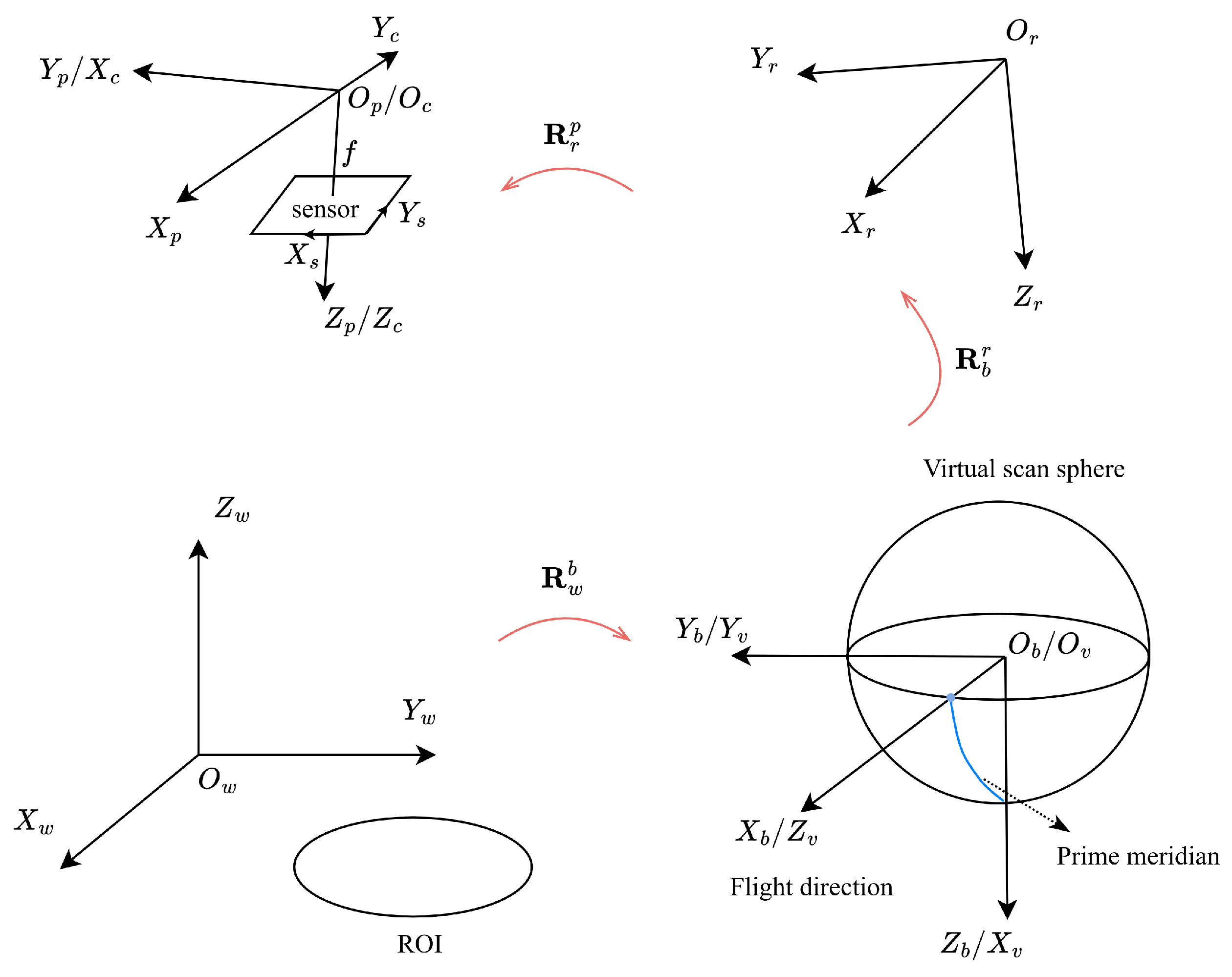
Figure 1 depicts a schematic diagram of a step-stare imaging system. The system is mounted on an airborne platform and utilizes two-axis motors to drive an optical assembly for periodic rapid scans of single or multiple ROIs. During each step, the servos maintain a constant line-of-sight (LOS) orientation, allowing the area scan camera to stare at the target area. At the end of each scan cycle, the images from each stare are stitched together to form a single large-FOV equivalent image. The center of all the footprints form a grid graph. Definitions of the relevant coordinate systems can be found in Appendix A. The main notations adopted in this study are listed in Table A1.
We should mention that this paper makes the following assumptions: (a) During a scan, the center of the projection undergoes no translational motion, and the heading angle remains constant based on the fact that step-stare optical systems are typically driven by high-torque motors, resulting in fast LOS movement. (b) The gimbal configuration of the imaging system has two axes, with the outermost axis being the roll axis and the innermost axis being the pitch axis. This configuration is commonly used for wide-area imaging systems. (c) The aircraft attitude is disregarded because gyro-attitude stabilizers can typically achieve stabilization accuracy within [35]. (d) The shape of the ROI is a circle or convex polygon. (e) The profile of the camera sensor (such as CCD or CMOS) is a non-square rectangle. (f) The ROI is located on a planar surface, i.e., variations in terrain undulations and the curvature of the earth are not taken into account.
Based on the given assumptions, each camera sensor’s ground footprint is a quadrilateral region created by the projection of the camera sensor onto the ground. It is the intersection of the quadrangular pyramid formed by the camera’s FOV and the ground. The closed region determined by the footprint is defined as a cell and denoted as (i refers to the index).
where denotes the projective transformation from to , S denotes the camera sensor’s geometry, denotes the coordinates of the origin of in , denotes the ith orientation of the camera, and is the camera calibration matrix:
where f is the camera’s focal length, and represents the coordinates of the camera’s principal point. From Equation (1), we can infer that the shape of the cell correlates with the orientation of the camera at each step.
3.2. Problem Formulation
Let denote an ROI. The coverage path planning problem involves finding a set of camera orientations () and an optimal rotation path, with the goal of minimizing the path length and maximizing the coverage completeness of . The optimization problem can be decomposed into a path planning problem and a coverage planning problem, which are illustrated in Figure 2.
3.2.1. Path Planning Problem
The camera orientations of an ROI can be represented as a undirected weighted graph (, where element of is the vertex, and the path length between and is the edge ()). The label of each is defined as follows:
The goal is to minimize the path length of camera rotation.
This is a traveling salesman problem (TSP), and there are numerous proven methods for solving it. Since the coverage area of a step-stare system increases superlinearly with the tilt angle, the observation nodes of the ROI are typically small-scale, making coverage planning more important than path planning.
3.2.2. Coverage Planning Problem
Let denote a cover of ROI, and we have the following:
We wish to optimize the approximation of to while minimizing the cardinality of .
where denotes the function that calculates the area, and is the hyperparameter of the penalty term. Fixing n relaxes this problem into a maximal coverage location problem (MCLP) [36], which is known to be NP-hard. Therefore, the coverage planning problem is NP-hard.
The NP-hard problem cannot be solved in polynomial time. To address this problem, our methodology involves using a low-complexity approximation method to obtain a locally optimal solution. This approach provides a “good-enough” solution and may even reach the global optimum in some cases.
4. Proposed Method
The proposed method is detailed in this section. A complete flowchart of the algorithm is depicted in Figure 3, comprising three main modules. During the initialization phase, the ROI parameters, the camera’s parameters, and the necessary rotation matrix are prepared, and the radius of the virtual scanning sphere is calculated. These parameters are then provided to the coverage planning module. To achieve complete coverage of an ROI, we present a seamless hyperbolic grid (SHG) based on zonal isosceles trapezoids. Then, we propose a novel dual-caliper optimization (DCO) algorithm for circular and polygonal regions, which yields a more compact set of camera orientations. Finally, a rotation path is determined using the bound-and-branch method and the boustrophedon method.
4.1. Seamless Hyperbolic Grid
Conventional methods for coverage planning typically assume vertical imaging situations, where the camera’s ground footprint is rectangular, similar to the frame sensor. Such a grid has a rectangular geometry and can easily be used for planar tiling. However, determining a seamless tiling grid from the perspective of Euclidean geometry is not convenient for a step-stare imaging system with rotational motion. Inspired by the tiling (tessellation) problem, the completeness of coverage is investigated from a perspective of spherical tiling. Here, the term tiling (tessellation) refers to covering of a surface by one or more geometric shapes with no gaps or overlaps.
Several studies have been conducted on spherical tiling problems in astronomy, geosciences, astronautics, and multi-camera stitching [37,38,39,40,41]. However, they usually focus on equal-area or Platonic polyhedron tiling, which do not consider the projective geometric properties of the sensor. Next, the spherical tiling problem of a rectangular sensor’s projections is discussed in detail.
4.1.1. Equivalent Spherical Tiling
Step-stare motion covers a spherical space, so a virtual scanning sphere (VSS) is defined to represent this.
Definition 1.
A virtual scanning sphere of a camera is a sphere centered at the origin of the camera coordinate system such that it touches each of the camera sensor’s vertices, regardless of the camera’s orientation. It can be expressed as follows:
where f is the focal length of the camera, and and are the width and height of the sensor, respectively. We denotes the radius of the VSS as .
A VSS of a single-lens camera is illustrated in Figure 4a. The sensor plane, the VSS, and the ROI plane are isomorphic because the central projection between them is a homograph. Thus, we can convert the ROI’s complete covering problem into an equivalent spherical tiling problem, that is, by finding a set of such that
where is the sensor’s image of , and is the ROI’s image of . Since the sensor’s FOV can be considered a non-square rectangular pyramid, the contour of is a spherical quadrilateral. In particular, it has equal opposite sides, unequal adjacent sides, and equal interior angles that are greater than . This shape is defined as a spherical pseudo rectangle (SPR). The following theorem holds for SPRs:
Theorem 1.
Congruent SPRs cannot achieve spherical tiling.
Proof.
Suppose there exists a spherical region that can be tiled by a number of congruent SPRs. Let the interior angle of an SPR be , and let the degree of one of the vertices in this tiling pattern be ; then, is satisfied. Since , we get , i.e., the vertex is trivalent. In this case, there are only four possible edge combinations (aaaa, aaab, aabb, and aabc) for a spherical quadrilateral [42]. Since the edge combination of an SPR is abab, a contradiction arises.
Figure 5a depicts the abab edge combination of an SPR. The straight line segments (a and b) depicted in the figure are, in fact, geodesic segments on the sphere. Figure 5b illustrates one possible SPR tiling pattern in which the longer edge serves as a common side. In this way, a third SPR () has an edge combination where two edges (a) are adjacent. This contradicts the fact that an SPR must be in a form of and that two edges (a) should be separate. A similar contradiction can be observed in the other SPR tiling pattern, as illustrated in Figure 5c. □
Theorem 1 claims that for a step-stare imaging system with a non-square rectangular sensor, there exists no that can make the corresponding camera footprints a tiling of the ROI’s neighborhood. Thus, alternative approximation methods need to be found to achieve seamless coverage.
4.1.2. Approximate Tiling Method
As can be seen from Figure 4a, given a VSS with a camera sensor oriented towards , the corners on the sensor’s base side determine an arc of a parallel (line of latitude), while the corners on the leg determining an arc of a great circle. By referencing the definition of an spherical isosceles trapezoid [43], we define the geometry formed by these four arcs as a zonal isosceles trapezoid (ZIT).
Definition 2.
A spherical quadrilateral is called a zonal isosceles trapezoid if one pair of its opposite sides are arcs of parallels and the other pair are symmetric geodesics.
Given a ZIT, we call the arc of a parallel a base and the arc of a geodesic a leg.
Inspired by recursive zonal equal-area partition [44], we align a set of camera sensors on a parallel of a VSS, naming the set of their orientations a zonal cover (denoted by ). In this way, the envelope of these sensors’ corners forms a ZIT (denoted by ). Let be the union of all (the ith sensor’s projection on VSS) in a zonal cover and be the maximal inscribed ZIT of . The relationship between , , and is illustrated in Figure 6.
For a ZIT, we have the following theorem:
Theorem 2.
Given a VSS and a separate ROI, there exists a set of ZITs on the VSS such that the union of contains , namely , where denotes the ROI’s image of and denotes the region enclosed by the ZIT ().
Proof.
is bounded in a hemisphere () of the VSS, i.e., . A set of adjacent is arrange along the meridional direction without gaps (as shown in Figure 4b) such that the latitude range of is greater than . Then, the width of each is adjusted such that the longitude range of is greater than . In this way, we can make the hemisphere a subset of , i.e., . □
According to Theorem 2, we need to further investigate the following two problems:
- How to determine each roll angle (or latitude) of a sensor in a zonal cover ();
- How to determine each pitch angle (or longitude) of the zonal cover () in the meridional direction.
4.1.3. Zonal Arrangement
We propose the arrangement of zonal in such a way that the low-latitude sides of adjacent sensors are connected side by side, as shown in Figure 6a. Then, we obtain the recursive formula for each in as follows:
where is the low latitude of the corresponding that is also the latitude of a ZIT’s base, and is an indicator function that indicates is larger than .
From Equation (9c), we can deduce that , which means that the FOVs of adjacent sensors overlap. Thus, this method provides an approximate tiling. The approximation error converges as the absolute latitude value decreases.
4.1.4. Meridional Arrangement
The goal of meridional arrangement is to find a recursive formula to tiling each zonal cover’s along the meridional direction.
Given a zonal cover and an attached camera, for a point (A) on a sensor’s base, we have the following equation according to Proposition A2:
where is the latitude of A; is the latitude of the midpoint (M) of the base; and d is the Euclidean distance from A to M, i.e., . When , reaches the minimum value, at this time the point, A is a corner of the sensor. Let denote the corner’s latitude; then, we have the following:
According to the definitions of and ZIT, a sensor’s corner always lies on the base line of ; thus, we have the following:
where is the latitude of a ZIT’s base.
Let denote the spherical region enclosed by . Then, based on Equations (11) and (12), we can obtain the latitude range of (denoted by ) as follows:
where the subscripts N and S denote the northern and southern part, respectively.
Combined with Equation (9c), can be expressed as follows:
where is the radius of VSS, and and are the minimum and maximum longitude of , respectively.
The latitude () of the ith zonal cover is defined as the latitude of its attached sensor’s center; then we have the following:
where is the sensor’s FOV along the axis.
Given a pair of adjacent zonal covers aligned in the meridional direction, let and denote the indices of relative high-latitude (closer to the poles) and relative low-latitude (closer to the equator) cover, respectively. According to Equation (13), if two can be tiled along meridional direction, then the following equations must hold:
Therefore, a recursive formula of can be obtained by combining Equations (11), (15), and (16) as follows:
where is the indicator function that determines whether is .
4.1.5. Hyperbolic Grid
Since a set of can form a tiling on a VSS, the projection of the corresponding sensor centers on the ground forms a grid graph. Given a parallel of a VSS with a latitude of , its conic coefficient matrix on the plane ( in ) can be expressed as follows:
Under a point transformation (), a conic can be transformed as follows:
where is the projection of on the ground.
By considering the transformation as an imaging process, the finite projective camera model can be used to obtain [45] as follows:
where is the elevation value of the ROI in , and is the inhomogeneous coordinate of in . Since is related to the attitude of the aircraft, we can infer from knowledge of conic curves that the shape of could be all kinds of conic curves, i.e., ellipse, parabola, and hyperbola. But under the assumptions presented in Section 3, we can ignore the effect of the aircraft’s attitude; thus, takes the form of a hyperbola. Therefore, by using the approximate tiling method, the centers of each camera ground footprint are located on a bundle of hyperbolas, forming a seamless hyperbolic grid (SHG).
4.2. Dual-Caliper Optimization
As described above, a seamless hyperbolic grid ensures coverage completeness. However, to reduce the number of step-stare steps and shorten the path length, the grid layout needs further optimization. For this purpose, we propose a novel dual-caliper optimization (DCO) method. Before that, we present the necessary definitions, which are illustrated in Figure 7.
Definition 3.
A supporting hyperbola of a convex set (P) is a hyperbola with one of its branches (B) passing through a point of P so that the interior of P lies entirely on one side of B and the corresponding focus lies on the opposite side. Point C is called a support point.
Definition 4.
An extreme hyperbola is a supporting hyperbola that is a projection of the VSS’s parallel.
Definition 5.
A zonal slice of a convex set (P) is a closed region covered by the central projection of a spherical zone of a VSS.
Definition 6.
Given a zonal slice (Z) of a convex set (P), the partial boundary shared by Z and P is called the slice boundary.
Definition 7.
An extreme orientation of a zonal cover () is an element of such that the projection of its corresponding camera sensor’s vertical outer sideline admits a supporting line of a zonal slice formed by the extended base of .
According to the definition of zonal cover, the extreme orientation has the following property:
Property 1.
Given a zonal cover (), the longitude (ϕ) of an extreme orientation is either the maximum or the minimum of all the longitudes in .
In this section, we first obtain the extreme hyperbola of the ROI and determine the optimal arrangement of the zonal covers based on the latitude range. Then, the extreme orientation of each zonal cover is calculated and the zonal stride is optimized. The method described above involves solving for the supporting hypersurface (i.e., supporting hyperbola and supporting line) in both meridional and zonal directions, which resembles using two types of calipers to measure the size of the ROI. Therefore, we name this method dual-caliper optimization (DCO), as shown in Figure 7a, inspired by the rotating caliper algorithm [46] in computational geometry.
4.2.1. Meridional Curved Caliper
In the first phase of DCO, we use a meridional curved caliper to determine two extreme hyperbolas of an ROI. Specific geometric algorithms differ depending on the shape of the ROI, such as circular or convex polygonal, based on the assumptions presented in Section 3. It is worth noting that a hyperbola mathematically has two branches, only one of which is the true projection of the parallel on the sphere, called the valid branch in this paper, while the other one is called the fake branch.
(1) For a circular ROI:
The conic matrix of a circular ROI on the ground can be expressed as follows:
where is the center, and is the radius. The goal is to solve such that the following simultaneous equations have only one real solution:
where represents the homogeneous coordinates of a point on the ground. The above system of equations means that (the image of under ) and are tangent, and they form a quartic equation with nonlinear terms of unknown , which is difficult to solve. We employ a numerical method to cope with this problem.
All linear combinations of the conics that pass through the intersection of and can be represented by a bundle of conics (). We now search for a suitable such that is degenerate, which means that it can be factorized into a product of two linear polynomials over a complex field. The discriminant of a degenerate conic equals zero.
This equation is essentially a cubic equation with three solutions in the complex plane. According to the fundamental theorem of algebra, a cubic equation with an unknown has at least one real root. This means that at least one degenerate conic in the bundle () is real. In this way, a real line pair can be decomposed from by a method introduced in [47]. Let consist of two distinct lines, namely and , as follows:
The adjoint of is
According to the definition of cross product, is the intersection of lines and . Let ; then, can be represented as the definition of a cross product as follows:
Now, we obtain , where the subscript denotes the index of any non-zero diagonal element in , and denotes the ith column of . It can be derived that the skew-symmetric matrix () of is . Combining Equation (25), we have the following:
where is a square matrix with rank = 1. Then, by selecting any non-zero element in , we can find the homogeneous coordinates for and as the corresponding row and column of , respectively.
To solve for the intersection point () of line (resp. ) and circle , we first extract two different arbitrary points ( and ) from (resp. ); then, can be expressed as . Since is a symmetric square matrix, we obtain a quadratic equation with an unknown k, as follows:
If the above equation has two conjugate complex solutions, then there is no real intersection between line (or ) and circle . On the other hand, two distinct real solutions indicate that they intersect at two real points, and one real repeated root means they are tangent. If a real solution exists, we can calculate the corresponding latitude () of using Equation (A4) and compare it with the of . If and only if they are equal, the intersection is on the valid branch, and the circular ROI intersects the hyperbola of .
By performing the above steps iteratively using binary search, we can obtain a that forms an extreme hyperbola of the ROI. The Algorithm 1 pseudocode is presented below. represents the search interval, and set can be considered the “sign” indicating whether and intersect. Figure 8a provides a clear illustration of this algorithm. Since the aperture angle of the ROI () is less than (i.e., ), the following propositions hold: and guarantee and will not intersect, while guarantees intersection. The algorithm repeatedly bisects the interval in two directions, as illustrated by the arrows, until the interval is sufficiently small. Subsequently, we obtain the solution of . The red hyperbolas represent the solution’s corresponding .
| Algorithm 1: Meridional Curved Caliper Algorithm for a Circular ROI |
 |
(2) For convex polygonal ROIs:
Figure 8b provides an illustration of this algorithm for convex polygonal ROIs. Given a convex polygon (), the procedure to determine the latitude () of the extreme hyperbola is as follows. First, we compute the latitude of all vertices of by using Equation (A4) and select the vertex with the largest (resp. smallest) latitude (), as denoted by . Next, the projection () on the ground corresponding to is obtained by Equations (19) and (20). Finally, using Equation (29), we can determine the intersection of with and , which are the adjacent line segments of . If there exists no real solution other than , then is the latitude of the extreme hyperbola, as shown in Figure 9a. Otherwise, based on Theorem 3, we further derive two candidate solutions numerically such that the corresponding valid branch of the hyperbola is tangent to and (as shown in Figure 9b), respectively. Finally, the largest (resp. smallest) value of these two candidates is selected as the latitude of an extreme hyperbola.
Theorem 3.
Given a VSS, a convex polygon (), and a vertex (V) of with the maximum or minimum latitude, an extreme hyperbola of must either pass through V or be tangent to one of its adjacent edges, without exception.
Proof.
Figure 9 illustrates the projection of a bundle of parallels of a VSS. The hyperbolas closer to the upper side correspond to larger latitudes (and vice versa). Let be the vertex in with the largest latitude in , and let be an adjacent vertex whose corresponding latitude is no greater than that of . Let be an open line segment, and let denote the hyperbola that passes through . Only two possible topological relations exist between and . The first is that and have no intersection (as shown in Figure 9a) in such a way that becomes an extreme hyperbola (). The second is that and have one intersection, which lies in , as shown in Figure 9b. In the latter case, there must exist a hyperbola with a greater latitude than , which is tangent to . Similarly, the above conclusion holds for the vertex with the smallest latitude. □
4.2.2. Meridional Stride Optimization
The two extreme hyperbolas of the ROI determine the minimum requirement of the meridional FOV to cover the ROI. Moreover, the latitudes of the corresponding extreme zonal covers, denoted by and , can be derived by using the equations presented in Section 4.1.4. Since is the optimal meridional covering range, the meridional stride between adjacent zonal covers can be further optimized.
First, we compute the size (n) of . By starting from and following Equation (17) based on a seamless hyperbolic grid, we obtain the latitude of each recursively until it exceeds the northernmost bound (); then, the iteration count is n. By adding a refinement term () to Equation (17), the optimization of meridional stride becomes equivalent to finding a suitable that satisfies the following equation:
where , and is the recursive operator in Equation (17). This is essentially a nested nonlinear equation. Since is a function of and is monotone in the range of , the root can be solved by a numerical method such as binary search.
4.2.3. Zonal Straight Caliper
After meridional stride optimization, we can collect a set of zonal covers with determined latitudes (). Next, we aim to solve the optimal range of longitude () for each zonal cover (). Given a zonal cover () and a zonal slice () enclosed by the projection of ’s spherical zone, we define the zonal straight caliper of as a pair of supporting lines, which are the projections of the camera sensor’s outer vertical sideline on the ground, as shown in Figure 7a. In such case, the orientation of the camera is the extreme orientation (Definition 7), and the supporting line is called an extreme line. The corresponding extreme orientations of the zonal straight caliper determine the minimum zonal FOV to cover the zonal slice.
The algorithm of a zonal straight caliper consists of the following three steps: (1) Find all candidate support points on the slice boundary. (2) Select the support point from the candidates. (3) Obtain the longitude of extreme orientation based on the support point. It is worth noting that the specific methods in step 1 and step 2 depend on the ROI’s geometry.
Step 1: For a circular ROI, the slice boundary is an arc, and the candidate support point could be either the endpoint of the arc or the point at which the arc and the supporting line are tangent. For a convex polygonal ROI, the slice boundary is a polygonal chain; then, the candidate support point could be any vertex in the chain.
Step 2: For a circular ROI, according to Proposition A3, we can determine if each endpoint () of the slice boundary is the support point. If neither is the support point, binary search can be used to find such that the projection of a camera sensor’s outer vertical sideline and the slice boundary are tangent, where and are as follows:
where , , , and are the four corner points of the sensor represented by homogeneous coordinates in , which indicate the top right, bottom right, bottom left, and top left, respectively. is a sign function that indicates ’s position in the zonal slice, with a value of 1 if on the left flank and otherwise.
For a convex polygonal ROI, Property 1 is referenced as the rule used to select a support point from candidates.
Step 3: According to Equation (9c), we can calculate the longitude () of an extreme orientation based on the support point () as follows:
where is the latitude–longitude coordinate of in , which can be calculated by Equation (A4).
4.2.4. Zonal Stride Optimization
After obtaining the longitudinal bound () for (subscripts W and E denote the zonal direction of the bound), further optimization of the zonal stride is needed to make the zonal cells more compact.
When using the default longitude step () of the seamless hyperbolic grid in Equation (9c), the number of camera sensors () in is expressed as follows:
Thus, the optimal longitudinal step () is expressed as follows:
Then, the optimized recursive formula of the longitude of each camera in a zonal cover is as follows:
4.3. Path Planning
After determining the optimized coverage of the ROI, a rotation path should be provided such that the optical system performs a “stare” at each orientation step. For scenarios requiring periodic visits, the path must be a closed loop. In this case, path planning is equivalent to the symmetric traveling salesman problem (TSP). The TSP can be characterized as a Dantzig–Fulkerson–Johnson (DFJ) model [48] as follows, where Equation (37d) stipulates that no subtour is allowed for this path.
where is a binary variable indicating whether there is a path from to , and represents the distance between and . For a step-stare system, since the motors of the pitch and roll gimbals are driven simultaneously during each step movement, we adopt the Chebyshev distance () as follows:
The TSP is an integer programming problem that can be solved using exact, approximation, or heuristic algorithms. Among them, branch and bound is a commonly used exact algorithm to provide an exact solution and has been adopted in many modern TSP solvers [49]. Considering that the step scale is typically small in most scenarios, we use branch and bound as the planning method for closed paths.
In some scenarios, it may be necessary to visit multiple ROIs sequentially, leading to an open-form path for each ROI. To generate such a path, we utilize the boustrophedon method. This facilitates the fast motion of the optical servo in a single direction and simplifies the mechanism for image smear compensation.
5. Results
This section introduces the dataset setup and experimental evaluation metrics, followed by an ablation experiment to verify the necessity of each component in the proposed method. Finally, we evaluate several typical coverage path planning methods for performance comparison.
5.1. Experimental Setup and Dataset Generation
In order to fulfill the typical requirements of wide-area persistent surveillance, the parameters were initially set according to the specifications outlined in Table 1. The camera parameters (focal length, pixel size, and number of pixels) were selected based on off-the-shelf uncooled long-wave infrared cameras. The spatial resolution threshold value was chosen as the lowest threshold that is acceptable for state-of-the-art computer vision algorithms to detect moving targets such as vessels and vehicles. In addition, the heading angle of the UAV was set to a fixed initial value of , and the ground elevation was set to zero for convenience of calculation. Given that the ROIs are randomly generated, the heading angle setting of the UAV does not influence the experimental conclusions.
As shown in Figure 10, the ROI () is limited to a circle () defined by the parameters listed in Table 1, namley , where is the planar coordinate of in . The radius () can be calculated using basic trigonometry and the pinhole camera model as follows:
where b is the pixel size, h is the relative height, is the spatial resolution threshold of the LOS, and f is the camera’s focal length. As indicated by Equation (39), the variables b and h are inversely related to , while f and are positively related to . It should be noted that these parameters only affect the position and geometry of the generated ROIs utilized in this experiment.
The dataset of the ROI consists of two categories, namely circles and convex polygons, each of which is generated randomly within . For a circular ROI, we employ the candidate radius sampling strategy [50]; the process is illustrated in Figure 11a. First, the radius () is randomly sampled in to provide scale variation, where the lower bound is designed to prevent the generation of a tiny ROI. Next, the polar coordinates of the center are generated randomly within the range of to ensure adequate location diversity. For a convex polygonal ROI, we create a random number of points within , then compute the convex hull, as shown in Figure 11b. Each convex polygon sample is determined by a set of Cartesian coordinates of the vertices.
Moreover, the ROI should be large enough to prevent the algorithms from generating insufficient cells, which would lead to ineffective performance comparisons. For this purpose, we pre-screened the synthetic samples using our proposed AHG method to discard samples with fewer than 6 cells or more than 15 cells. Finally, the ROIs in the dataset were categorized into 10 groups based on the number of cells in our proposed algorithm’s results, and 40 ROI samples were retained for each group.
5.2. Evaluation Metric
Regarding performance evaluation, we utilize the three most commonly used metrics for coverage path planning, namely path length (PL), coverage rate (CR, denoted as ), and computation time (CT). Specifically, PL uses the Chebyshev distance to evaluate the angular traveling length, while CT uses CPU consumption time to evaluate the algorithm’s complexity. characterizes the completeness of ROI coverage, which is defined as follows:
Moreover, we introduce an additional metric, namely the number of cells (NC), which also represents the number of steps. Clearly, NC affects the complexity of the servo control algorithm and the update frequency of the panorama imagery of the system.
5.3. Ablation Study
As mentioned above, this paper presents a coverage path planning method with adaptive hyperbolic grid (AHG). It consists of two main components: seamless hyperbolic grid (SHG) and dual calipers optimization (DCO). SHG achieves complete coverage (i.e., CR = 1) for any bounded ROI, while DCO approximates the ROI with variable quadrilaterals and compresses the grid’s scale. To evaluate the benefits of these two components, we designed the ablation experiment by replacing SHG in the proposed method with a fixed-step grid and replacing DCO with a scanline-based flood fill. Experiments were performed on our synthetic ROI dataset. Metrics of and NC are utilized for comparison; here, refers to statistical probability.
Table 2 presents the statistical results of . The method with DCO alone achieves 98.0% and 97.5% complete coverage on each category, indicating its ability to provide seamless coverage in most but not all cases. On the other hand, the method with SHG consistently achieves remarkable 100% on all samples, proving its effectiveness as a means of achieving complete coverage.
The quantitative result of NC for the circle and convex polygon categories is visualized in Figure 12, with lower values indicating better results. Let the method without SHG and DCO serve as the baseline. It can be observed that the proposed AHG (with SHG and DCO) can achieve the best performance on all datasets. Compared to the baseline, using only SHG improved NC by an average of 5.1% and 1.2% for each category, respectively. In contrast, the DCO-only method significantly improves them by an average of 26.4% and 30.4%, achieving the second-best results. Notably, the performance with only DCO approaches the best level. This indicates that the DCO component can better exploit the geometry correlation between the cells, thus optimizing the grid scale more effectively.
5.4. Performance Comparison with Other Methods
This subsection evaluates the efficiency of various algorithms using our custom ROI dataset, which comprises diverse geometries. All the methods involved were implemented in Matlab R2022b, and the experiments were conducted on an off-the-shelf computer with an AMD Ryzen 5 7500F CPU.
The ROIs were utilized as inputs to the algorithms, which output LOS orientations to create closed-form and open-form paths. Each LOS corresponds to an image obtained from a single exposure. More specifically, to validate the performance of the proposed AHG method, we compared its experimental results with three typical coverage planning methods, namely flood fill (FF) [51], particle swarm optimization (PSO) [33], and replanning sidewinder (RS) [31]. The flood fill algorithm is commonly utilized for coverage path planning on a rectangular grid with uniformly fixed strides. In this experiment, we set the stride of to . In addition, we adopt the efficient scan-line strategy and use collision detection to determine if the camera footprint meets the boundary of the ROI. PSO is a no-decomposition method that models the coverage problem as a mixed-integer optimization problem and iteratively searches for the optimal solution using a particle swarm. This algorithm may consume a large number of iterations, especially if the number of cells that need to be optimized is a variable. In contrast to [33], which ignores this parameter, we use the result generated by our approach as the upper bound, then perform a binary search to iterate the PSO and determine the optimal value. Moreover, the cost function is defined as , and the threshold is set to 2%. Replanning sidewinder is an approach of approximate cellular decomposition. Since the original article [31] did not mention either the size of the cell or the specific numerical algorithm for optimizing the grid origin, we adopted the camera’s nadir footprint and chose the commonly used golden ratio search algorithm to remove taboo tiles and prevent revisiting of a previous cell.
For path planning, we use both the boustrophedon and branch-and-bound methods for evaluation, except for PSO, which exclusively employs the branch-and-bound method because of its metaheuristic nature and non-parameterizable grid. In particular, both opposite scanning directions are evaluated in boustrophedon, and the path with the shortest length is selected as the final result.
Figure 13a,b provide the results of boustrophedon path length comparison between the proposed AHG method, FF, and RS. We find that AHG achieves the best result in all data groups. In the circle category, AHG reduces the path length remarkably by an average of 43.71% and 30.41% compared to FF and RP, respectively. In the convex polygon category, the average improvement gains are 47.31% and 26.35%, respectively. Figure 13c,d present the comparison results of path length generated by the branch-and-bound method. Our proposed AHG method outperforms FF and RP excessively, with relative gains of 42.62% and 27.29% in the circle category and 38.61% and 16.71% in polygon category, respectively. Compared to PSO, the performance of our method is slightly inferior by an overall average of 4.32% and 6.71% in each category but performs better by 6.75% and 2.3% for groups 1 and 6 in the circle category, respectively, and by 0.13% for group 1 of the polygon category. It is shown that although the proposed AHG is a rule-based method, it achieves superior path length relative to heuristic optimization in a few scenarios.
Table 3 shows the comparison results of coverage rate. To prevent misinterpretation due to quantization errors, the mean value was truncated to one decimal place, while the standard error was rounded up to one decimal place. We can observe that both AHG and RP can achieve a 100% coverage ratio on every sample. However, AHG achieves this through a simple, seamless hyperbolic grid, while RP employs tedious one-dimensional cell searching at the expense of a higher NC. Moreover, neither the FF nor the PSO methods can achieve complete coverage for every dataset. This is mainly due to the fact that FF employs fixed strides that cannot ensure overlapping FOVs of adjacent sensors, while the PSO method aims to optimize coverage with a certain cost threshold, resulting in the coverage of gaps caused by convergent residuals. Additionally, the average CR residual of PSO exceeds 2% in group 3 of the circle category, indicating that PSO fails to reach a globally optimal solution that meets the threshold requirement within the maximum number of iterations.
According to the NC comparison in Table 4, PSO outperforms all other methods on all datasets due to its global optimization mechanism. AHG is ranked first alongside PSO in two groups (1 and 6) of the circle category and ranked second in the remaining groups. This is mainly because it is an approximation method for coverage planning, providing a local optimal solution in a constrained search space. On the other hand, FF yielded unsatisfactory results due to the lack of a grid optimization scheme, and the NC of RP was negatively affected by the disparity between the camera ground footprint and the fixed-size cell.
Table 5, Table 6 and Table 7 summarize the comparison results of coverage computation time (CCT), overall computation time with boustrophedon path planning (OCTB), and overall computation time with branch-and-bound path planning (OCTBB), respectively. Here, the overall computation time involves both coverage planning and path planning. Among the compared approaches, AHG achieves the best in CCT, OCTB, and OCTBB among all categories. This is mainly due to the fact that AHG only imposes the computational burden of calculating the boundary of each zonal slice. In contrast, FF must compute the collision between each cell and the ROI, RP must determine taboo tiles and optimize cells’ origins for each cell commitment, and PSO is required to explore the ROI with a sizable particle swarm. Furthermore, it can be observed from Table 5 that AHG has a worst CCT of only 12.7 ms, indicating that it provides real-time planning capability. In contrast, PSO has an optimal CCT of 31.3 s, making it suitable only for offline scenarios.
For visual comparison, the coverage paths of four methods are shown in Figure 14, where the circular and polygonal ROIs are colored red, the cells (camera footprints) are colored blue, and the paths generated by the boustrophedon and branch-and-bound methods are highlighted with red bold lines. The figures demonstrate that the cells produced by AHG are more compact than those generated by FF and RS and comparable to those generated by PSO. Figure 14a,e clearly depict the effect of dual-caliper optimization, as the aligned zonal covers’ projections approximate the ROI in the heading direction and “clamp” each zonal slice in the cross direction. Particularly, in the circle category, our AHG method achieves the same optimal cell count as PSO but with a superior path length. Figure 14b,f demonstrate that the FF method produces redundant cells due to a lack of optimization for ROI. It also has a negative effect on the scanning rate. Figure 14c,g illustrate that the NC obtained by the PSO method is optimal. However, the non-uniform stride of the cells prevents parameterization, making PSO inapplicable for boustrophedon path planning methods. Figure 14d,h indicate that the RS method generates redundant cells due to improper approximate cellular decomposition.
This experiment validates the efficiency and low complexity of this algorithm with a customized dataset in the dimensions of ROI shape, viewing distance, and size. However, it should be noted that there are some limitations when applying our method. (1) This method is more suitable for circular ROIs and convex polygonal ROIs and does not currently support concave polygonal or annular ROIs. (2) This method is more suitable for “bird’s-eye-view” flying scenarios at relatively high altitudes. It does not, however, address the issue of occlusion that is often encountered when a UAV flies at low altitudes.
6. Conclusions
This paper proposes a novel coverage path planning method with an adaptive hyperbolic grid (AHG) for step-stare imaging systems. The key points of this method are to arrange each stare by constructing an approximate tiling in a virtual spherical space and compress the hyperbolic grid by measuring the scale with dual calipers. First of all, to address the issue of coverage completeness, we convert the coverage problem in Euclidean space to a tiling problem in spherical space. A virtual scanning sphere model is constructed, and an approximate tiling by spherical zonal isosceles trapezoid is proposed to achieve seamless coverage planning. Next, to further optimize the grid layout, we propose a dual-caliper optimization method by exploiting the geometry correlation between conic and convex polygons. Experiments based on diverse geometries and viewpoints demonstrate that the proposed AHG method can achieve complete coverage for circular and convex polygonal ROIs and exhibits competitive performance with low computational complexity. Additionally, this study provides researchers with a novel perspective for solving the coverage planning problem in the case of rotational motion. This method could be applied to many practical applications besides WAPS, including robot sensing [52], mass and slope movement monitoring [53,54], and ecological observation [55].
Although the proposed method’s effectiveness and efficiency were validated through comprehensive experiments and analysis, there are still some issues that require further discussion in the future.
- We constrained a step-stare imaging system with basic pitch and roll axes. However, for multi-axis systems with additional gimbals or mechanical linkage, the orientation of the sensor’s footprint can be adjusted with more degrees of freedom, which can further optimize the grid layout. The coverage optimization of a multi-axis system will be studied in the future.
- We assumed the carrier platform moves at a slow speed and the position of the camera is stationary during the scanning process. However, for vehicle carriers that exhibit high-speed maneuvering, the hyperbolic grid becomes time-varying, which may invalidate the coverage path plan. Further investigation is needed to design efficient coverage path planning methods in such scenarios.
- In path planning, we chose the simple Chebyshev distance as a metric. But in engineering applications, the trajectory of gimbals is usually optimized as a smooth curve [56] (e.g., Bezier curve, Dubins curve, etc.). Therefore, in future studies, the curve path length should be considered as the evaluation metric.
- The obstacle effect represents a significant factor in the planning process. When an obstacle is present in the field of view, the target area may become a concave set due to occlusion. In future work, we will incorporate obstacle effect constraints into the optimization problem and investigate the coverage planning problem in this context.
Funding
This research received no external funding.
Institutional Review Board Statement
Not applicable.
Informed Consent Statement
Not applicable.
Data Availability Statement
The data presented in this study are available upon request from the corresponding author.
Acknowledgments
We would like to express our gratitude to Chunlei Yang for his valuable assistance in developing the prototype of the optoelectronic system.
Conflicts of Interest
Author Jiaxin Zhao was employed by the company Changchun Changguang Insight Vision Optoelectronic Technology Co., Ltd. The remaining authors declare that the research was conducted in the absence of any commercial or financial relationships that could be construed as a potential conflict of interest.
Abbreviations
The following abbreviations are used in this manuscript:
| AHG | Adaptive hyperbolic grid |
| CCT | Coverage computation time |
| CPP | Coverage path planning |
| CR | Coverage rate |
| CT | Computation time |
| DCO | Dual-caliper optimization |
| DOF | Degrees of freedom |
| FF | Flood fill |
| FOV | Field of view |
| LOS | Line of sight |
| PSO | Particle swarm optimization |
| PL | Path length |
| ROI | Region of interest |
| RS | Replanning sidewinder |
| SHG | Seamless hyperbolic grid |
| SPR | Spherical pseudo rectangle |
| TSP | Traveling salesman problem |
| UAV | Unmanned aerial vehicle |
| VSS | Virtual scanning sphere |
| WAPS | Wide-area persistent surveillance |
| ZIT | Zonal isosceles trapezoid |
Appendix A. Coordinate Systems and Transformations
The coordinate systems defined in this paper are presented in this section. With the assumptions in Section 3, , , , , and have origins identical origins to that of the ideal center of projection of the optical system, as illustrated in Figure A1.
World coordinate system () is defined as a Cartesian coordinate system for a local region of the Earth’s surface where the curvature of the Earth can be ignored. The axis faces upwards. The and axes are located on the surface of the region of interest.
A body coordinate system () is used to represent the outer frame of the step-stare imaging system. represents the roll axis of the step-stare imaging system and generally runs in the flight direction. represents the azimuth axis.
A virtual scanning sphere coordinate system () is a latitude–longitude coordinate system. With reference to , we define , , and . The intersections of the axis and the virtual scanning sphere are defined as the north pole and south pole such that the north pole (resp. south pole) is in the positive (resp. negative) direction of . The prime meridian is defined as the intersection of the plane and the lower hemisphere.
A roll gimbal coordinate system () is a coordinate system used to represent the roll-axis frame. The rotation matrix from to is expressed as follows:
where is the roll angle of the step-stare system.
A pitch gimbal coordinate system () is a coordinate system used to represent the pitch-axis frame. The rotation matrix from to is expressed as follows:
where is the pitch angle of the step-stare system.
A camera coordinate system () represents the frame of a camera. The sensor lies in the plane of . The relation between and is expressed by , , and . The rotation matrix from to is expressed as follows:
A sensor coordinate system () is a 2D coordinate frame used to define a rectangular sensor such as CCD or CMOS, where the origin is at the top-left corner of the sensor, and the (resp. ) axis is oriented in the same direction as (resp. ).
Figure A1.
Coordinate systems and transformations.
Appendix B. Symbol Notation
The main notations used throughout this paper are listed in Table A1.

Table A1.
Symbol notation.
| Symbol | Description |
|---|---|
| Coordinate system | |
| Projective mapping between different | |
| Projective matrix between different | |
| Rotation matrix between different | |
| Cell, i.e., enclosed area defined by the camera’s ground footprint | |
| Pitch gimbal angle or latitude | |
| Roll gimbal angle or longitude | |
| f | Focal length |
| Sensor’s horizontal field of view | |
| Sensor’s vertical field of view | |
| The width of the sensor | |
| The height of the sensor | |
| Sensor’s orientation expressed by gimbal angles | |
| A set of | |
| A zonal set of | |
| Calibration matrix | |
| P | A given region’s image of on a sphere |
| The ith sensor’s projection on a sphere | |
| The union of all in a zonal cover | |
| The zonal isosceles trapezoid determined by sensors’ corner envelope | |
| The maximal inscribed zonal isosceles trapezoid of | |
| Homogeneous coordinates of a point | |
| Inhomogeneous coordinates of a point |
Appendix C. Supplementary Propositions
Proposition A1.
Given a point () in , its latitude and longitude in can be calculated as follows:
where is the inhomogeneous coordinate of a point in , is the inhomogeneous coordinate of in , and is the rotation matrix from to .
Proposition A2.
Given a sphere with center O, let be a chord of a small circle with the center (N) and let M be a midpoint of , as shown in Figure A2. Then, we have the following:
Proof.
From Figure A2, we can observe that , , and . □
Figure A2.
Proposition A2.

Proposition A3.
Given a VSS, a circular region (), a zonal slice (), and a supporting line () of with support point , let be an intersection point of and the extended base of except . Then, must not be inside the ROI.
Proof.
Let the projection of the corresponding spherical zone of be , and we have the following:
Since is on the supporting line of but is not the support point, we have . And since lies in the extended base of and , we have . Now, we can deduce the following:
so we have . □
References
- Cobb, M.; Reisman, M.; Killam, P.; Fiore, G.; Siddiq, R.; Giap, D.; Chern, G. Wide-area motion imagery vehicle detection in adverse conditions. In Proceedings of the 2023 IEEE Applied Imagery Pattern Recognition Workshop (AIPR), Saint Louis, MO, USA, 27–29 September 2023; pp. 1–6. [Google Scholar] [CrossRef]
- Negin, F.; Tabejamaat, M.; Fraisse, R.; Bremond, F. Transforming temporal embeddings to keypoint heatmaps for detection of tiny Vehicles in Wide Area Motion Imagery (WAMI) sequences. In Proceedings of the IEEE 2022 IEEE/CVF Conference on Computer Vision and Pattern Recognition Workshops (CVPRW), New Orleans, LA, USA, 19–20 June 2022; pp. 1431–1440. [Google Scholar] [CrossRef]
- Sommer, L.; Kruger, W.; Teutsch, M. Appearance and motion based persistent multiple object tracking in Wide Area Motion Imagery. In Proceedings of the 2021 IEEE/CVF International Conference on Computer Vision Workshops (ICCVW), Montreal, BC, Canada, 11–17 October 2021; pp. 3871–3881. [Google Scholar] [CrossRef]
- Li, X.; He, B.; Ding, K.; Guo, W.; Huang, B.; Wu, L. Wide-Area and Real-Time Object Search System of UAV. Remote. Sens. 2022, 14, 1234. [Google Scholar] [CrossRef]
- Luo, X.; Zhang, F.; Pu, M.; Guo, Y.; Li, X.; Ma, X. Recent Advances of Wide-Angle Metalenses: Principle, Design, and Applications. Nanophotonics 2021, 11, 1–20. [Google Scholar] [CrossRef]
- Driggers, R.; Goranson, G.; Butrimas, S.; Holst, G.; Furxhi, O. Simple Target Acquisition Model Based on Fλ/d. Opt. Eng. 2021, 60, 023104. [Google Scholar] [CrossRef]
- Stamenov, I.; Arianpour, A.; Olivas, S.J.; Agurok, I.P.; Johnson, A.R.; Stack, R.A.; Morrison, R.L.; Ford, J.E. Panoramic Monocentric Imaging Using Fiber-Coupled Focal Planes. Opt. Express 2014, 22, 31708. [Google Scholar] [CrossRef] [PubMed]
- Huang, Y.; Fu, Y.; Zhang, G.; Liu, Z. Modeling and Analysis of a Monocentric Multi-Scale Optical System. Opt. Express 2020, 28, 32657. [Google Scholar] [CrossRef] [PubMed]
- Yuan, X.; Ji, M.; Wu, J.; Brady, D.J.; Dai, Q.; Fang, L. A Modular Hierarchical Array Camera. Light Sci. Appl. 2021, 10, 37. [Google Scholar] [CrossRef] [PubMed]
- Daniel, B.; Henry, D.J.; Cheng, B.T.; Wilson, M.L.; Edelberg, J.; Jensen, M.; Johnson, T.; Anderson, S. Autonomous collection of dynamically-cued multi-sensor imagery. In Proceedings of the SPIE Defense, Security, and Sensing, Orlando, FL, USA, 13 May 2011; p. 80200A. [Google Scholar]
- Kruer, M.R.; Lee, J.N.; Linne Von Berg, D.; Howard, J.G.; Edelberg, J. System considerations of aerial infrared imaging for wide-area persistent surveillance. In Proceedings of the SPIE Defense, Security and Sensing, Orlando, FL, USA, 13 May 2011; p. 80140J. [Google Scholar]
- Driggers, R.G.; Halford, C.; Theisen, M.J.; Gaudiosi, D.M.; Olson, S.C.; Tener, G.D. Staring Array Infrared Search and Track Performance with Dither and Stare Step. Opt. Eng. 2018, 57, 1. [Google Scholar] [CrossRef]
- Driggers, R.; Pollak, E.; Grimming, R.; Velazquez, E.; Short, R.; Holst, G.; Furxhi, O. Detection of Small Targets in the Infrared: An Infrared Search and Track Tutorial. Appl. Opt. 2021, 60, 4762. [Google Scholar] [CrossRef]
- Sun, J.; Ding, Y.; Zhang, H.; Yuan, G.; Zheng, Y. Conceptual Design and Image Motion Compensation Rate Analysis of Two-Axis Fast Steering Mirror for Dynamic Scan and Stare Imaging System. Sensors 2021, 21, 6441. [Google Scholar] [CrossRef]
- Xiu, J.; Huang, P.; Li, J.; Zhang, H.; Li, Y. Line of Sight and Image Motion Compensation for Step and Stare Imaging System. Appl. Sci. 2020, 10, 7119. [Google Scholar] [CrossRef]
- Fu, Q.; Zhang, X.; Zhang, J.; Shi, G.; Zhao, S.; Liu, M. Non-Rotationally Symmetric Field Mapping for Back-Scanned Step/Stare Imaging System. Appl. Sci. 2020, 10, 2399. [Google Scholar] [CrossRef]
- Miller, J.L.; Way, S.; Ellison, B.; Archer, C. Design Challenges Regarding High-Definition Electro-Optic/Infrared Stabilized Imaging Systems. Opt. Eng. 2013, 52, 061310. [Google Scholar] [CrossRef]
- Choset, H. Coverage for Robotics—A Survey of Recent Results. Ann. Math. Artif. Intell. 2001, 31, 113–126. [Google Scholar] [CrossRef]
- Galceran, E.; Carreras, M. A Survey on Coverage Path Planning for Robotics. Robot. Auton. Syst. 2013, 61, 1258–1276. [Google Scholar] [CrossRef]
- Cabreira, T.; Brisolara, L.; Ferreira, P.R., Jr. Survey on Coverage Path Planning with Unmanned Aerial Vehicles. Drones 2019, 3, 4. [Google Scholar] [CrossRef]
- Tan, C.S.; Mohd-Mokhtar, R.; Arshad, M.R. A Comprehensive Review of Coverage Path Planning in Robotics Using Classical and Heuristic Algorithms. IEEE Access 2021, 9, 119310–119342. [Google Scholar] [CrossRef]
- Đakulovic, M.; Petrovic, I. Complete Coverage Path Planning of Mobile Robots for Humanitarian Demining. Ind. Robot. Int. J. 2012, 39, 484–493. [Google Scholar] [CrossRef]
- Acar, E.U.; Choset, H.; Zhang, Y.; Schervish, M. Path Planning for Robotic Demining: Robust Sensor-Based Coverage of Unstructured Environments and Probabilistic Methods. Int. J. Robot. Res. 2003, 22, 441–466. [Google Scholar] [CrossRef]
- Latombe, J.C. Robot Motion Planning; Springer Science & Business Media: Berlin/Heidelberg, Germany, 2012; pp. 206–207. [Google Scholar]
- Choset, H.; Pignon, P. Coverage path planning: The boustrophedon cellular decompositio. In Field and Service Robotics; Springer: London, UK, 1998; pp. 203–209. [Google Scholar]
- Coombes, M.; Fletcher, T.; Chen, W.-H.; Liu, C. Optimal Polygon Decomposition for UAV Survey Coverage Path Planning in Wind. Sensors 2018, 18, 2132. [Google Scholar] [CrossRef]
- Tang, G.; Tang, C.; Zhou, H.; Claramunt, C.; Men, S. R-DFS: A Coverage Path Planning Approach Based on Region Optimal Decomposition. Remote Sens. 2021, 13, 1525. [Google Scholar] [CrossRef]
- Nam, L.; Huang, L.; Li, X.J.; Xu, J. An approach for coverage path planning for UAVs. In Proceedings of the 2016 IEEE 14th International Workshop on Advanced Motion Control (AMC), Auckland, New Zealand, 22–24 April 2016; pp. 411–416. [Google Scholar]
- Cao, Y.; Cheng, X.; Mu, J. Concentrated Coverage Path Planning Algorithm of UAV Formation for Aerial Photography. IEEE Sens. J. 2022, 22, 11098–11111. [Google Scholar] [CrossRef]
- Shang, Z.; Bradley, J.; Shen, Z. A Co-Optimal Coverage Path Planning Method for Aerial Scanning of Complex Structures. Expert Syst. Appl. 2020, 158, 113535. [Google Scholar] [CrossRef]
- Shao, E.; Byon, A.; Davies, C.; Davis, E.; Knight, R.; Lewellen, G.; Trowbridge, M.; Chien, S. Area coverage planning with 3-axis steerable, 2D framing sensors. In Proceedings of the Scheduling and Planning Applications Workshop, International Conference on Automated Planning and Scheduling, Delft, The Netherlands, 26 June 2018. [Google Scholar]
- Vasquez-Gomez, J.I.; Marciano-Melchor, M.; Valentin, L.; Herrera-Lozada, J.C. Coverage Path Planning for 2D Convex Regions. J. Intell. Robot. Syst. 2020, 97, 81–94. [Google Scholar] [CrossRef]
- Mansouri, S.S.; Kanellakis, C.; Georgoulas, G.; Kominiak, D.; Gustafsson, T.; Nikolakopoulos, G. 2D Visual Area Coverage and Path Planning Coupled with Camera Footprints. Control. Eng. Pract. 2018, 75, 1–16. [Google Scholar] [CrossRef]
- Papaioannou, S.; Kolios, P.; Theocharides, T.; Panayiotou, C.G.; Polycarpou, M.M. Integrated Guidance and Gimbal Control for Coverage Planning With Visibility Constraints. IEEE Trans. Aerosp. Electron. Syst. 2022, 59, 1–15. [Google Scholar] [CrossRef]
- Li, S.; Zhong, M. High-Precision Disturbance Compensation for a Three-Axis Gyro-Stabilized Camera Mount. IEEE/ASME Trans. Mechatron. 2015, 20, 3135–3147. [Google Scholar] [CrossRef]
- Megiddo, N.; Zemel, E.; Hakimi, S.L. The Maximum Coverage Location Problem. SIAM J. Algebr. Discret. Methods 1983, 4, 253–261. [Google Scholar] [CrossRef]
- Zhang, X.; Zhao, P.; Hu, Q.; Ai, M.; Hu, D.; Li, J. A UAV-Based Panoramic Oblique Photogrammetry (POP) Approach Using Spherical Projection. ISPRS J. Photogramm. Remote Sens. 2020, 159, 198–219. [Google Scholar] [CrossRef]
- Beckers, B.; Beckers, P. A General Rule for Disk and Hemisphere Partition into Equal-Area Cells. Comput. Geom. 2012, 45, 275–283. [Google Scholar] [CrossRef]
- Liang, X.; Ben, J.; Wang, R.; Liang, Q.; Huang, X.; Ding, J. Construction of Rhombic Triacontahedron Discrete Global Grid Systems. Int. J. Digit. Earth 2022, 15, 1760–1783. [Google Scholar] [CrossRef]
- Li, G.; Wang, L.; Zheng, R.; Yu, X.; Ma, Y.; Liu, X.; Liu, B. Research on Partitioning Algorithm Based on Dynamic Star Simulator Guide Star Catalog. IEEE Access 2021, 9, 54663–54670. [Google Scholar] [CrossRef]
- Kim, J.-S.; Hwangbo, M.; Kanade, T. Spherical Approximation for Multiple Cameras in Motion Estimation: Its Applicability and Advantages. Comput. Vis. Image Underst. 2010, 114, 1068–1083. [Google Scholar] [CrossRef]
- Ueno, Y.; Yoshio, Y. Examples of Spherical Tilings by Congruent Quadrangles. In Memoirs of the Faculty of Integrated Arts and Sciences; IV, Science Reports; Hiroshima University: Hiroshima, Japan, 2001; Volume 27, pp. 135–144. [Google Scholar]
- Avelino, C.P.; Santos, A.F. Spherical F-Tilings by Scalene Triangles and Isosceles Trapezoids, I. Eur. J. Comb. 2009, 30, 1221–1244. [Google Scholar] [CrossRef]
- Leopardi, P. A Partition of the Unit Sphere into Regions of Equal Area and Small Diameter. Electron. Trans. Numer. Anal. 2006, 25, 309–327. [Google Scholar]
- Hartley, R.; Zisserman, A. Multiple View Geometry in Computer Vision, 2nd ed.; Cambridge University Press: New York, NY, USA, 2003; pp. 153–157. [Google Scholar]
- Toussaint, G. Solving geometric problems with the rotating calipers. In Proceedings of the 1983 IEEE MELECON, Athens, Greece, 24–26 May 1983. [Google Scholar]
- Richter-Gebert, J. Perspectives on Projective Geometry: A Guided Tour Through Real and Complex Geometry, 1st ed.; Springer: Berlin/Heidelberg, Germany, 2011; pp. 190–193. [Google Scholar]
- Dantzig, G.; Fulkerson, R.; Johnson, S. Solution of a Large-Scale Traveling-Salesman Problem. J. Oper. Res. Soc. Am. 1954, 2, 393–410. [Google Scholar] [CrossRef]
- Sanches, D.; Whitley, D.; Tinós, R. Improving an exact solver for the traveling salesman problem using partition crossover. In Proceedings of the 2017 Genetic and Evolutionary Computation Conference, Berlin, Germany, 15–19 July 2017; pp. 337–344. [Google Scholar]
- Tao, R.; Gavves, E.; Smeulders, A.W.M. Siamese instance search for tracking. In Proceedings of the 2016 IEEE Conference on Computer Vision and Pattern Recognition (CVPR), Las Vegas, NV, USA, 27–30 June 2016; pp. 1420–1429. [Google Scholar]
- He, Y.; Hu, T.; Zeng, D. Scan-flood fill (SCAFF): An efficient automatic precise region filling algorithm for complicated regions. In Proceedings of the 2019 IEEE/CVF Conference on Computer Vision and Pattern Recognition Workshops (CVPRW), Long Beach, CA, USA, 15–20 June 2019; pp. 761–769. [Google Scholar]
- Verma, V.; Carsten, J.; Ravine, M.; Kennedy, M.R.; Edgett, K.S.; Culver, A.; Ruoff, N.; Williams, N.; Beegle, L. How do we get robots to take self-portraits on Mars? Perseverance-ingenuity and curiosity selfies. In Proceedings of the 2022 IEEE Aerospace Conference (AERO), Big Sky, MT, USA, 5 March 2022; pp. 1–14. [Google Scholar]
- Urban, R.; Štroner, M.; Blistan, P.; Kovanič, Ľ.; Patera, M.; Jacko, S.; Ďuriška, I.; Kelemen, M.; Szabo, S. The Suitability of UAS for Mass Movement Monitoring Caused by Torrential Rainfall—A Study on the Talus Cones in the Alpine Terrain in High Tatras, Slovakia. ISPRS Int. J. Geo-Inf. 2019, 8, 317. [Google Scholar] [CrossRef]
- Núñez-Andrés, M.A.; Prades-Valls, A.; Matas, G.; Buill, F.; Lantada, N. New Approach for Photogrammetric Rock Slope Premonitory Movements Monitoring. Remote Sens. 2023, 15, 293. [Google Scholar] [CrossRef]
- Lyons, M.B.; Brandis, K.J.; Murray, N.J.; Wilshire, J.H.; McCann, J.A.; Kingsford, R.T.; Callaghan, C.T. Monitoring Large and Complex Wildlife Aggregations with Drones. Methods Ecol. Evol. 2019, 10, 1024–1035. [Google Scholar] [CrossRef]
- Mier, G.; Valente, J.; de Bruin, S. Fields2Cover: An Open-Source Coverage Path Planning Library for Unmanned Agricultural Vehicles. IEEE Robot. Autom. Lett. 2023, 8, 2166–2172. [Google Scholar] [CrossRef]
Figure 1.
Schematic diagram of step-stare imaging system.

Figure 2.
Formulation of the coverage path planning problem for step-stare imaging systems.

Figure 3.
Flowchart of our proposed AHG method.

Figure 4.
Virtual scanning sphere of a single-lens camera and zonal isosceles trapezoid. (a) The projection of the camera sensor forms a spherical pseudo rectangle. (b) A set of zonal isosceles trapezoids aligned in the meridional direction.
Figure 4.
Virtual scanning sphere of a single-lens camera and zonal isosceles trapezoid. (a) The projection of the camera sensor forms a spherical pseudo rectangle. (b) A set of zonal isosceles trapezoids aligned in the meridional direction.

Figure 5.
Spherical tiling of an SPR. (a) The edge combination of an SPR is . (b) Two SPRs are arranged with the longer edge serving as a common side. (c) Two SPRs are arranged with the shorter edge serving as a common side.
Figure 5.
Spherical tiling of an SPR. (a) The edge combination of an SPR is . (b) Two SPRs are arranged with the longer edge serving as a common side. (c) Two SPRs are arranged with the shorter edge serving as a common side.

Figure 6.
Zonal isosceles trapezoid (), the union of the sensor’s projection on a VSS (), and the maximal inscribed ZIT of (). (a) The envelope of the sensors’ corners forms a . (b) approximates the contour of . (c) is the maximal inscribed ZIT of .
Figure 6.
Zonal isosceles trapezoid (), the union of the sensor’s projection on a VSS (), and the maximal inscribed ZIT of (). (a) The envelope of the sensors’ corners forms a . (b) approximates the contour of . (c) is the maximal inscribed ZIT of .

Figure 7.
Definitions used in Section 4.2. (a) A circular ROI is clamped by a meridional curved caliper. A zonal slice with four corners (, , , and ) is a part of the ROI, cut by the projection of a spherical zone. The zonal slice is clamped by a zonal straight caliper. (b) The parallels determined by a zonal set of camera sensors enclose a spherical zone. The vertical outer camera has an extreme orientation such that its outer vertical side projects to a supporting line of a zonal slice.
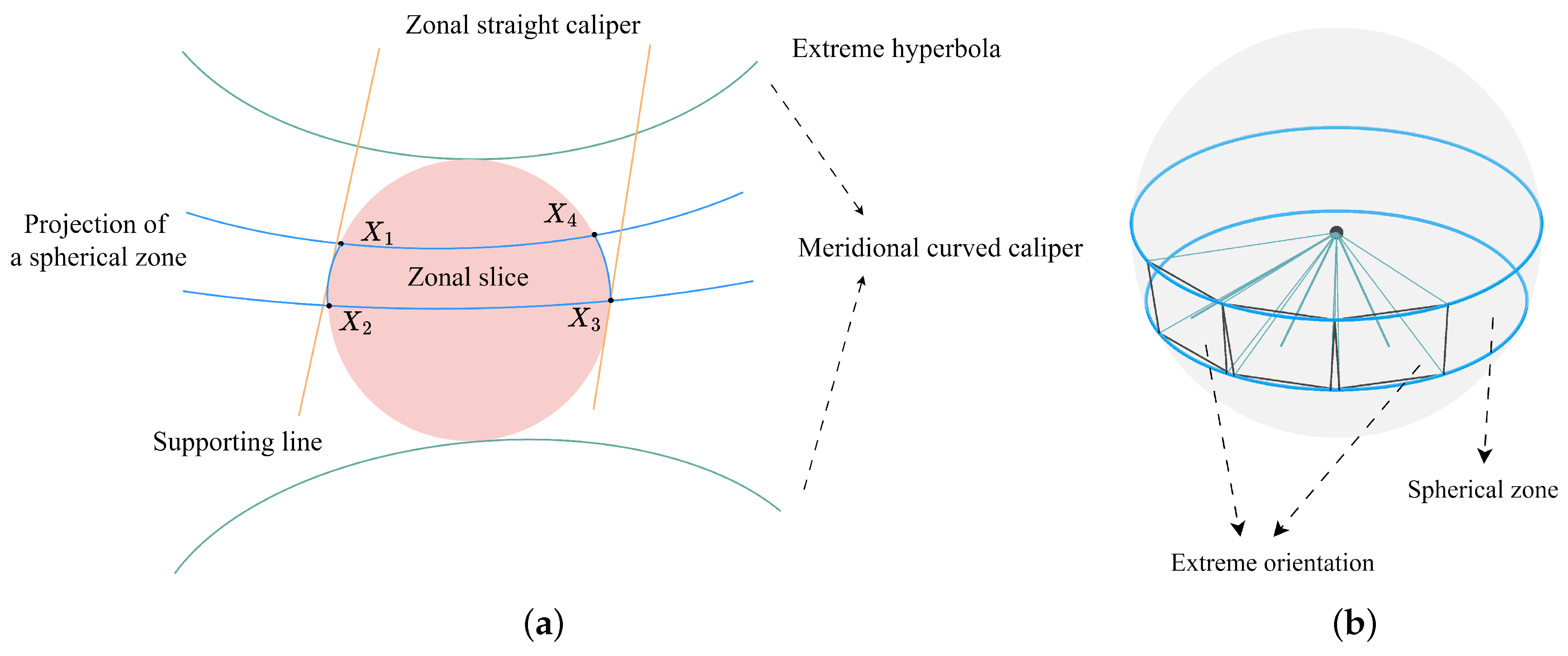
Figure 8.
Meridional curved caliper algorithm. (a) Circular ROI. (b) Convex polygonal ROI.

Figure 9.
The geometric relationship between a convex polygon and its extreme hyperbola. (a) The extreme hyperbola is the one that passes through . (b) The extreme hyperbola is tangent to an adjacent edge of .
Figure 9.
The geometric relationship between a convex polygon and its extreme hyperbola. (a) The extreme hyperbola is the one that passes through . (b) The extreme hyperbola is tangent to an adjacent edge of .

Figure 10.
The dataset is generated from defined by the experimental parameters.

Figure 11.
Dataset generation process. (a) Circular ROI generation. First, is generated from . Subsequently, are randomly sampled from . (b) Polygonal ROI generated by computing the convex hull of random points within .
Figure 11.
Dataset generation process. (a) Circular ROI generation. First, is generated from . Subsequently, are randomly sampled from . (b) Polygonal ROI generated by computing the convex hull of random points within .
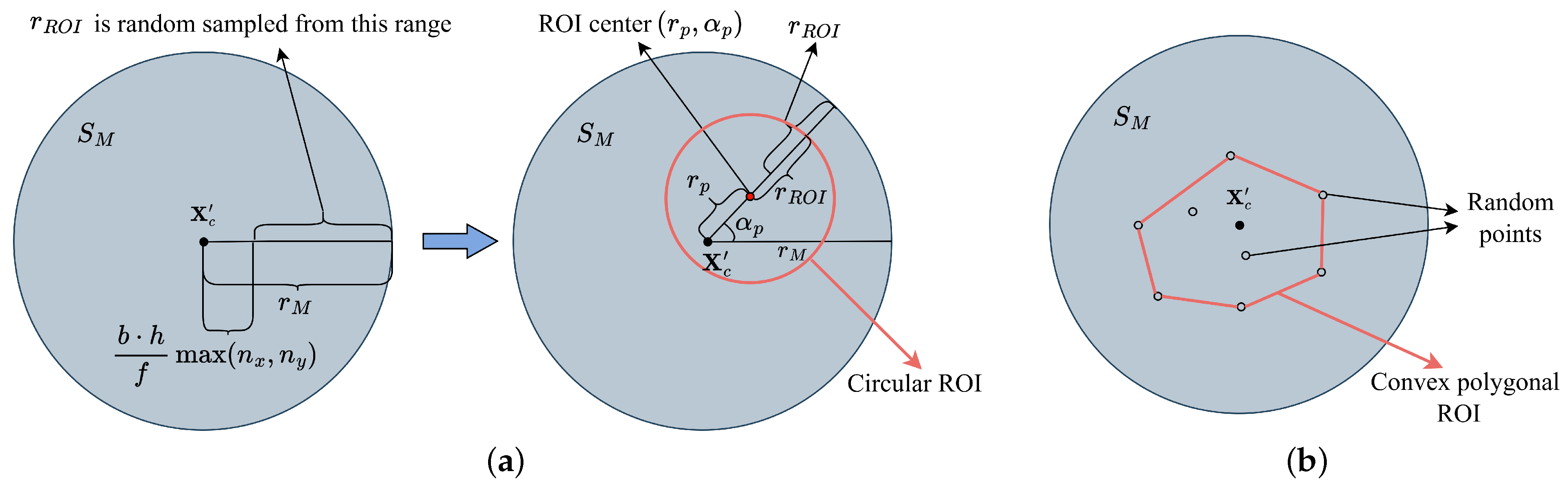
Figure 12.
The NC performance of the ablations on each component of DCO. A lower value is preferable. (a) Performance on the dataset with a circular ROI. (b) Performance on the dataset with a convex polygonal ROI.
Figure 12.
The NC performance of the ablations on each component of DCO. A lower value is preferable. (a) Performance on the dataset with a circular ROI. (b) Performance on the dataset with a convex polygonal ROI.
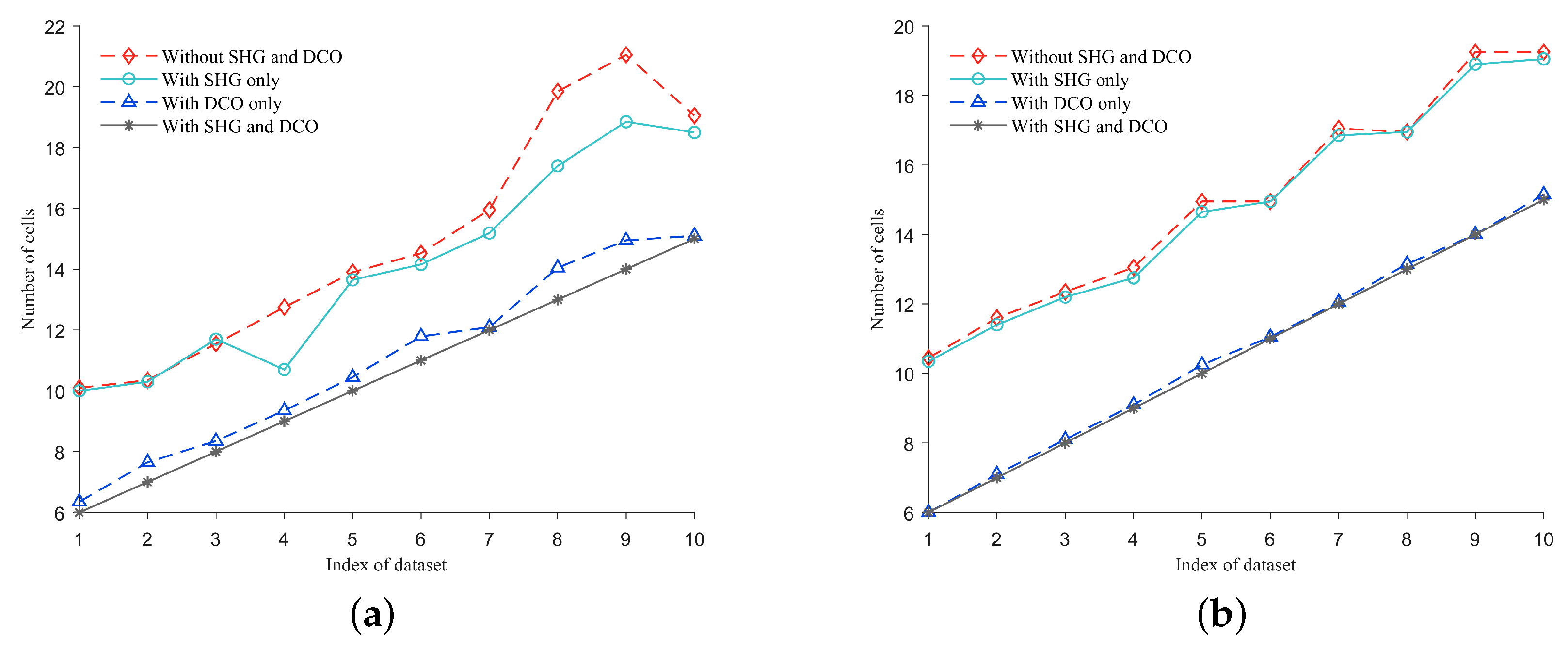
Figure 13.
Path length comparison results (lower values are preferable). (a) Boustrophedon path length in circle group. (b) Boustrophedon path length in convex polygon group. (c) Branch-and-bound path length in circle group. (d) Branch-and-bound path length in convex polygon group.
Figure 13.
Path length comparison results (lower values are preferable). (a) Boustrophedon path length in circle group. (b) Boustrophedon path length in convex polygon group. (c) Branch-and-bound path length in circle group. (d) Branch-and-bound path length in convex polygon group.
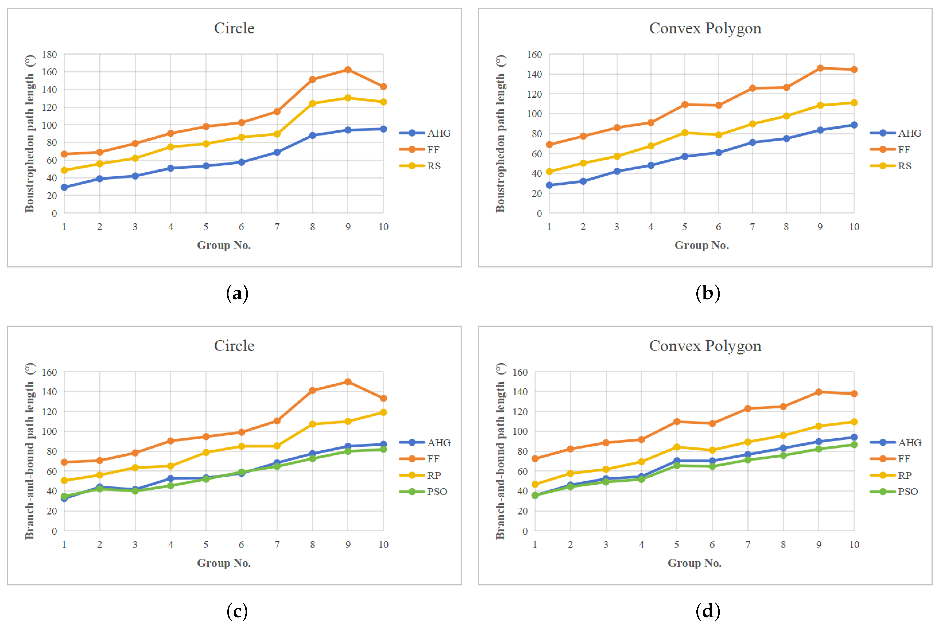
Figure 14.
Coverage path obtained via various methods. (a–d) The coverage cells and paths for a circular ROI generated by AHG, FF, PSO, and RS, respectively. The paths are produced by the brand-and-bound method. (e–h) The coverage cells and paths (except (g)) for a convex polygonal ROI generated by AHG, FF, PSO, and RS, respectively. The paths are produced by the boustrophedon method.

Table 1.
Experimental parameters.
| Parameter | Value |
|---|---|
| Focal length | 50 mm |
| Pixel size | 12 m |
| Number of pixels | |
| Relative height | 5000 m |
| Spatial resolution threshold * | 2 m |
* This threshold indicates the least acceptable spatial resolution.
Table 2.
Performance of on our synthetic dataset.
| SHG | DCO | Circular ROI | Convex Polygonal ROI |
|---|---|---|---|
| 69.5% | 42.0% | ||
| ✓ | 100.0% | 100.0% | |
| ✓ | 98.0% | 97.5% | |
| ✓ | ✓ | 100.0% | 100.0% |
Table 3.
Coverage rate (CR) performance of various methods.
| No. | Circle | Convex Polygon | ||||||
|---|---|---|---|---|---|---|---|---|
| AHG (%) | FF (%) | PSO (%) | RP (%) | AHG (%) | FF (%) | PSO (%) | RP (%) | |
| 1 | ||||||||
| 2 | ||||||||
| 3 | ||||||||
| 4 | ||||||||
| 5 | ||||||||
| 6 | ||||||||
| 7 | ||||||||
| 8 | ||||||||
| 9 | ||||||||
| 10 | ||||||||
The bold numbers represent the optimal results, while the underlined numbers represent suboptimal results.
Table 4.
Number of cells (NC) for various methods.
| No. | Circle | Convex Polygon | ||||||
|---|---|---|---|---|---|---|---|---|
| AHG | FF | PSO | RP | AHG | FF | PSO | RP | |
| 1 | ||||||||
| 2 | ||||||||
| 3 | ||||||||
| 4 | ||||||||
| 5 | ||||||||
| 6 | ||||||||
| 7 | ||||||||
| 8 | ||||||||
| 9 | ||||||||
| 10 | ||||||||
The bold numbers represent the optimal results, while the underlined numbers represent suboptimal results.
Table 5.
Coverage planning computation time performance of various methods.
| No. | Circle | Convex Polygon | ||||||
|---|---|---|---|---|---|---|---|---|
| AHG (ms) | FF (ms) | PSO (s) | RP (ms) | AHG (ms) | FF (ms) | PSO (s) | RP (ms) | |
| 1 | ||||||||
| 2 | ||||||||
| 3 | ||||||||
| 4 | ||||||||
| 5 | ||||||||
| 6 | ||||||||
| 7 | ||||||||
| 8 | ||||||||
| 9 | ||||||||
| 10 | ||||||||
The bold numbers represent the optimal results, while the underlined numbers represent suboptimal results.
Table 6.
Overall computation time (with boustrophedon) performance of various methods.
| No. | Circle | Convex Polygon | ||||
|---|---|---|---|---|---|---|
| AHG (ms) | FF (ms) | RS (ms) | AHG (ms) | FF (ms) | RS (ms) | |
| 1 | ||||||
| 2 | ||||||
| 3 | ||||||
| 4 | ||||||
| 5 | ||||||
| 6 | ||||||
| 7 | ||||||
| 8 | ||||||
| 9 | ||||||
| 10 | ||||||
The bold numbers represent the optimal results, while the underlined numbers represent suboptimal results.
Table 7.
Overall computation time (with branch and bound) performance of various methods.
| No. | Circle | Convex Polygon | ||||||
|---|---|---|---|---|---|---|---|---|
| AHG (ms) | FF (ms) | PSO (s) | RP (ms) | AHG (ms) | FF (ms) | PSO (s) | RP (ms) | |
| 1 | ||||||||
| 2 | ||||||||
| 3 | ||||||||
| 4 | ||||||||
| 5 | ||||||||
| 6 | ||||||||
| 7 | ||||||||
| 8 | ||||||||
| 9 | ||||||||
| 10 | ||||||||
The bold numbers represent the optimal results, while the underlined numbers represent suboptimal results.
Disclaimer/Publisher’s Note: The statements, opinions and data contained in all publications are solely those of the individual author(s) and contributor(s) and not of MDPI and/or the editor(s). MDPI and/or the editor(s) disclaim responsibility for any injury to people or property resulting from any ideas, methods, instructions or products referred to in the content. |
© 2024 by the author. Licensee MDPI, Basel, Switzerland. This article is an open access article distributed under the terms and conditions of the Creative Commons Attribution (CC BY) license (https://creativecommons.org/licenses/by/4.0/).
Share and Cite
MDPI and ACS Style
Zhao, J. Coverage Path Planning with Adaptive Hyperbolic Grid for Step-Stare Imaging System. Drones 2024, 8, 242. https://doi.org/10.3390/drones8060242
AMA Style
Zhao J. Coverage Path Planning with Adaptive Hyperbolic Grid for Step-Stare Imaging System. Drones. 2024; 8(6):242. https://doi.org/10.3390/drones8060242
Chicago/Turabian StyleZhao, Jiaxin. 2024. "Coverage Path Planning with Adaptive Hyperbolic Grid for Step-Stare Imaging System" Drones 8, no. 6: 242. https://doi.org/10.3390/drones8060242