Article

A New Method of UAV Swarm Formation Flight Based on AOA Azimuth-Only Passive Positioning

1
School of Mathematics & Computer Science, Wuhan Polytechnic University, Wuhan 430048, China
2
School of Electrical and Electronic Engineering, Wuhan Polytechnic University, Wuhan 430048, China
*
Author to whom correspondence should be addressed.
These authors contributed equally to this work.
Drones 2024, 8(6), 243; https://doi.org/10.3390/drones8060243
Submission received: 16 April 2024 / Revised: 26 May 2024 / Accepted: 29 May 2024 / Published: 4 June 2024

Abstract

:
UAV swarm passive positioning technology only requires the reception of electromagnetic signals to achieve the positioning and tracking of radiation sources. It avoids the active positioning strategy that requires active emission of signals and has the advantages of good concealment, long acting distance, and strong anti-interference ability, which has received more and more attention. In this paper, we propose a new UAV swarm formation flight method based on pure azimuth passive positioning. Specifically, we propose a two-circle positioning model, which describes the positional deviation of the receiving UAV using trigonometric functions relative to the target in polar coordinates. Furthermore, we design a two-step adjustment strategy that enables the receiving UAV to reach the target position efficiently. Based on the above design, we constructed an optimized UAV swarm formation scheme. In experiments with UAV numbers of 8 and 20, compared to the representative comparison strategy, the proposed UAV formation scheme reduces the total length of the UAV formation by 34.76% and 55.34%, respectively. It demonstrates the effectiveness of the proposed method in the application of assigning target positions to UAV swarms.

1. Introduction

UAV swarm formation flight involves multiple UAVs flying in a specific formation to achieve cooperative operation, task division, and information sharing. The technology has wide-ranging applications in military, civil, scientific research, and entertainment fields [1,2,3,4,5,6,7,8,9,10]. To control multiple UAVs in a specific formation, it is primum necessary to localize them [7]. In UAV localization studies, early approaches can be categorized as active localization methods. These methods locate targets by transmitting signals outward and receiving echo signals. Although this technique offers fast positioning speed, it is easy to detect and interfere with, thus affecting positioning accuracy [11,12]. In order to compensate for this drawback, passive localization methods have recently become more and more popular. Unlike active localization methods, which require the sending of signals, passive localization methods only require the receiving of electromagnetic signals in order to locate and track the source of radiation [13]. Depending on the radiation source information received by the UAV, a number of passive localization methods [4,14,15,16,17] have been developed. The method based on Angle of Arrival (AOA) [15,18] is particularly suitable for multi-UAV distributed systems due to its high positioning accuracy, anti-jamming performance, and lack of need for time synchronization of the receiving station.
Incorporating channel model considerations is crucial for accurate AOA-based positioning, as the air-to-ground (A2G) communication link properties can significantly impact the accuracy. Recent studies, such as those by Mao et al. (2023) [19] and Lyu et al. (2023) [20], highlight the importance of understanding the dynamic and nonstationary characteristics of A2G channels. These studies provide valuable insights into the path loss, shadowing, and multipath effects [16,21,22,23] encountered in UAV communications, which are essential for designing reliable UAV-based wireless communication systems.
Many UAV formation schemes based on passive positioning have been proposed [1,2,3,24,25,26,27,28]. Li et al. [3] proposed a moving target passive positioning method based on the A-optimization criterion. Li et al. [29] proposed a unified formulation to calculate the accuracy factor (DOP). Li et al. [24] proposed a passive UAV positioning model based on Monte Carlo strategy in the context of passive positioning, and provided a trajectory planning decision scheme based on predictive computation of predefined endpoint positions of deviating UAVs. Fu et al. [25] proposed an analytical geometry-based pure azimuth passive positioning UAV localization and adjustment scheme. No et al. [2] proposed a procedure to compute guidance commands for controlling the relative geometry of multiple UAVs in formation flight. Li et al. [1] proposed an intelligent algorithm that combines model predictive control and standoff algorithm to solve the trajectory planning problem that the UAVs may encounter when tracking moving targets cooperatively in complex 3D environments. Wu et al. [26] proposed a multi-UAV cluster control method based on improved artificial potential field (APF), using k-means method to integrate and optimize the attractive force between the UAVs and introducing the concept of virtual core to achieve cluster control and adaptive formation flight of multi-UAV. Liu et al. [27] provided a detailed survey of the operational techniques of multi-vehicle systems in a variety of environmental domains, focusing on formation control and cooperative motion planning, with particular emphasis on the use of flexible formation shapes to achieve collision avoidance for multi-vehicle systems. Although progress has been made with the methods described above, two main limitations remain. Firstly, they may produce multipath effects during signal propagation. That is, the signal undergoes reflection and refraction during the propagation process, resulting in changes in signal arrival time and direction. As a result, more than one path for the signal reaches the receiving station, which affects the positioning accuracy in practical applications. Secondly, many methods are complex and computationally intensive, requiring more computational resources and increasing the cost of schemes.
To alleviate the above problem, we propose a new UAV swarm formation flight method based on pure azimuth passive positioning. We first propose a two-circle localization model to describe the deviation of the receiving UAV relative to the target position using polar coordinates and trigonometric functions. To accomplish this, we changed the previous method in which one UAV transmits and multiple UAVs receive, enabling a receiving UAV to receive angle information from multiple transmitting UAVs simultaneously. After determining the initial position of the UAV that receives the signals, we further propose a two-step adjustment strategy that guides the receiving UAV to move to the specified target position. Specifically, in the first step, the receiving UAV first moves in a straight line along the direction of the transmitting signal of one transmitting UAV until the receiving angle is the middle of the target angle. In the second step, the receiving UAV then moves in a straight line along the direction of the transmitting signal of another transmitting UAV until the receiving angle matches the target angle. Based on the above design, we further develop a formation scheme for multiple UAVs to assign target positions using the Hungarian algorithm.
Compared to previous methods, the proposed method has four distinct advantages. Firstly, by designing a receiving station to receive angle information from multiple transmitting stations simultaneously, the proposed method can corroborate each other according to the angle relationship, greatly increasing the error tolerance rate and significantly reducing the effect of multipath effects. Secondly, the proposed localization model represents the complex signal processing process with a few simple mathematical expressions. It reduces the difficulty of system implementation and achieves accurate localization results. Thirdly, the proposed adjustment strategy can control the receiver UAV to move to the target position using angle information with only two linear motions, greatly reducing the computation required to control UAV movement. Fourthly, the proposed formation scheme significantly reduces the sum of trajectory lengths when assigning random target locations to individual UAVs. The proposed formation scheme is effective for any shape of UAV swarm formation. Without loss of generality, a circular formation will be described as an example in the following section.
The rest of the paper is organized as follows. In Section 2, we present our UAV swarm formation flight method, including the two-circle positioning model and two-step adjustment strategy. Section 3 details the experimental setup and validates our method through comparisons with a representative strategy. Section 4 discusses the implications, advantages, limitations, and future research directions of our findings. Finally, Section 5 summarizes the key contributions and potential practical impacts of our proposed methods.

2. The New UAVs Swarm Formation Flight Method

This paper presents a novel approach to UAV swarm formation flight. We first analyze the drawbacks of the trilateral positioning method in angle-based passive positioning. To overcome this problem, we propose a two-circle localization model based on analytical geometry and trigonometric function theory that realizes the real-time precise localization of the three transmitting signal UAVs to the passive receiving signal UAVs based on AOA. Second, we design a two-step adjustment strategy to guide the passive signal-receiving UAVs to move the target position through a two-step linear motion using only the AOA changes received by the signal-receiving UAV during the motion. Finally, an n × n matrix is constructed with the position coordinates of all UAVs and all target positions, and the overall shortest distance matching is obtained by the Hungarian algorithm. The meanings represented by the symbols involved in the paper are shown in Table 1. As shown in Figure 1a–c, the proposed UAV swarm formation method consists of three key components: UAV positioning, UAV adjustment, and UAV swarm formation. In UAV positioning, the receiving UAV measures angles α and β with respect to transmitting UAVs to determine its position using the two-circle positioning model, where r represents the distance to the target point and θ is the angle formed with respect to the reference axis. In UAV adjustment, the receiving UAV first moves to align with the direction defined by the signal at angle α 1 , then adjusts to align with the signal at angle α 2 , ensuring accurate positioning with minimal movement. In UAV swarm formation, as shown in Figure 1c, each UAV U i is assigned to a target position in a circular formation using the Hungarian algorithm to optimize the overall movement distance, with initial transmitting UAVs L 0 and L 1 assisting in localization.

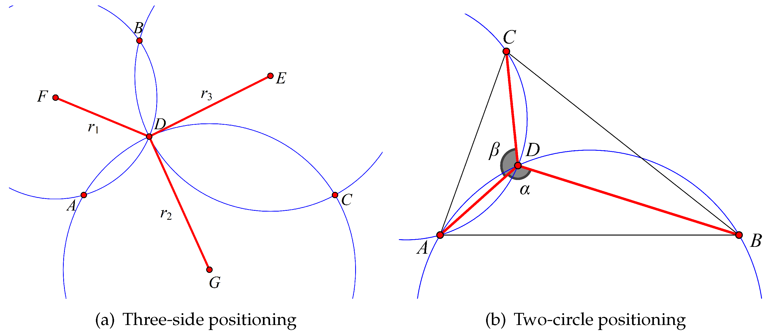
2.1. Two-Circle Positioning Model

A. Two-circle Positioning Principle
When the UAV swarm is attempting formation flight, in order to avoid external interference, it should maintain electromagnetic silence as much as possible and emit fewer electromagnetic wave signals to the outside. As a result, passive localization methods are becoming increasingly popular because they only require the reception of electromagnetic signals to locate and track the source of radiation. In particular, in the formation method based on pure azimuth passive positioning, it consists of a few UAVs being responsible for transmitting signals and the remaining UAVs passively receiving signals, from which the azimuth information is extracted for positioning and used to adjust the positions of the UAVs. Each UAV in the formation is assigned a fixed code number, and the relative position of each UAV to the others in the formation remains constant. As shown in Figure 2, the UAVs numbered FY01, FY02, and FY03 transmit signals, and the UAV numbered FY04 receives the azimuth information as α 1 , α 2 , and α 3 .
Among the previous positioning methods, the trilateral positioning method [30] is a representative one. Figure 3a shows the basic idea of the trilateral positioning method, in order to get the position of the unknown point D, we need to know the coordinates of three points, which are point E, point F and point G, meanwhile, we also need to know the distances from the unknown point D to the three points (E, F, G), which are the straight lines | E D | , | F D | and | G D | . Compared to the distance information of the three sides, the angle information between the three transmitting UAVs and the receiving UAV is more convenient to obtain and has a higher positioning accuracy. Therefore, in order to construct a pure azimuthal passive localization model, it is required to improve trilateration by using the angle information.
As shown in Figure 3b, the coordinates of the three transmitting UAVs and the angle α and β are known when the receiving UAV at point D can measure the angles ( α , β and B D C ) between three sides through the three transmitting UAVs. We can easily compute the coordinates of the intersection of the two circles by using the representations for the two outer circles, i.e., A and D. Where intersection point A is the location of the transmitting UAV that can be ruled out, intersection point D is the location of the receiving UAV. Therefore, under this hypothetical condition, the positioning can be done by using only the geometric relationship between the two circles. Also, this proves that at least three transmitting UAVs are needed for localization under this hypothetical condition.
B. Two-circle Positioning Model
Based on the above discussion, we propose a two-circle positioning model. As shown in Figure 4a, the two-circle positioning model of the receiving UAV is established by the position relationships between the points. Suppose the UAVs at point A, point B, and point C in the formation transmit signals; the UAV at point D receives signals; and the point O is the target position of the receiving UAV. The polar coordinate system is established with the point A as the origin and A B as the positive direction of the polar coordinate axis. Where the angle O A B formed between A O and A B is denoted by θ 0 , the angle D A O formed between A D and A O is denoted by θ and the angle between O D and A O is denoted by θ . D is on a circle with O as the center and r as the radius. The polar coordinates of the receiving UAV at point D are ρ , θ + θ 0 , the polar coordinates of the transmitting UAV C are r C , θ C , and the polar coordinates of the target point O are r 0 , θ 0 .
From the azimuth information received by the receiving UAV, we can obtain the angle information A D B and A D C , denoted by α and β , respectively. In D A O , according to the cosine theorem, the cosine representation for angle D A O is given by:
cos θ = D A 2 + O A 2 D O 2 2 D A · O A , = ρ 2 + ρ 0 2 r 2 2 ρ ρ 0 .
So,
ρ 2 2 ρ 0 ρ cos θ + ρ 0 2 r 2 = 0 .
In A D B , according to the sine theorem of the triangle, we can obtain the representation as:
D B sin D A B = A B sin A D B .
When we draw the perpendicular line from the point D to the line A B and intersect A B at point E. By the relationship between polar coordinates and Cartesian coordinates, the Cartesian coordinates of point E can be obtained by converting its polar coordinates, which yields ( ρ cos θ + θ 0 , ρ sin θ + θ 0 ). Then, A E = ρ cos θ + θ 0 and D E = ρ sin θ + θ 0 can be obtained.
In B D E , according to the Pythagorean Theorem, we can obtain the following representation as:
D B = D E 2 + E B 2 , = ρ sin θ + θ 0 2 + ρ B ρ cos θ + θ 0 2 , = ρ 2 + ρ B 2 2 ρ B ρ cos ( θ + θ 0 ) .
Combining Equations (3) and (4), we can obtain representation as:
ρ 2 + ρ B 2 2 ρ B ρ cos ( θ + θ 0 ) sin θ + θ 0 = ρ B sin α .
Similarly, in A C D , according to the sine theorem of the triangle, we can obtain representation as:
ρ 2 + ρ C 2 2 ρ ρ C cos θ C θ θ 0 sin θ C θ 0 θ = ρ C sin β .
However, it is not sufficient to use only Equations (5) and (6) for two-circle positioning, which may lead to the two-solution problem. As shown in Figure 4b, in the case where the line A D is perpendicular to the line C B , the angle α is complementary to the angle α and the angle β is complementary to the angle β , thus making the sine of α equal to the sine of α and the sine of β equal to the sine of β , resulting in a situation where two pairs of circles with the same radius can be made and the coordinates of the intersection points resulting from these two pairs are not the same, i.e., resulting in two solutions. To avoid this situation, we further restrict on A D C and A D B .
In A D B , according to the cosine theorem of the triangle, the cos α can be represented as:
cos α = A D 2 + B D 2 A B 2 2 · A D · B D , = ρ ρ B cos ( θ + θ 0 ) ρ 2 + ρ B 2 2 ρ B ρ cos ( θ + θ 0 ) .
Similarly, in A D C , according to the cosine theorem of the triangle, then the cos β can be represented as:
cos β = ρ ρ C cos ( θ C θ θ 0 ) ρ 2 + ρ C 2 2 ρ ρ C cos θ C θ θ 0 .
Combining Equations (5)–(8), the position of the receiving UAV at point D can be determined based on the azimuth information obtained from the passively received signal of the UAV at point D. Thus, the positioning model of the receiving UAV in the polar coordinate system with point A as the origin and A B as the polar coordinate axis can be represented as:
sin α = ρ B sin θ + θ 0 ρ 2 + ρ B 2 2 ρ B ρ cos ( θ + θ 0 ) , sin β = ρ C sin θ C θ 0 θ ρ 2 + ρ C 2 2 ρ ρ C cos θ C θ θ 0 , cos α = ρ ρ B cos ( θ + θ 0 ) ρ 2 + ρ B 2 2 ρ B ρ cos ( θ + θ 0 ) , cos β = ρ ρ C cos ( θ C θ θ 0 ) ρ 2 + ρ C 2 2 ρ ρ C cos θ C θ θ 0 .
In turn, the four conditions can be converted into two conditions by trigonometry as:
tan α = ρ B sin θ 0 + θ ρ ρ B cos θ 0 + θ , tan β = ρ C sin θ C θ 0 θ ρ ρ C cos θ C θ 0 θ .
From Equation (10), we can find ρ and θ so that we can determine the positioning coordinates of the receiving UAV as ρ , θ 0 + θ . Using the target point O as the origin and A O as the polar axis, a new polar coordinate system is established. Bringing in ρ and θ , the representation of r and θ can be obtained as:
r = ρ 2 2 ρ 0 ρ cos θ + ρ 0 2 , θ = θ θ π arc cos ρ 0 2 + r 2 ρ 2 2 r · ρ 0 .
Finally, in the coordinate system with the target point O as the origin and A O as the polar axis, the positioning coordinate of the receiving UAV is r , θ .

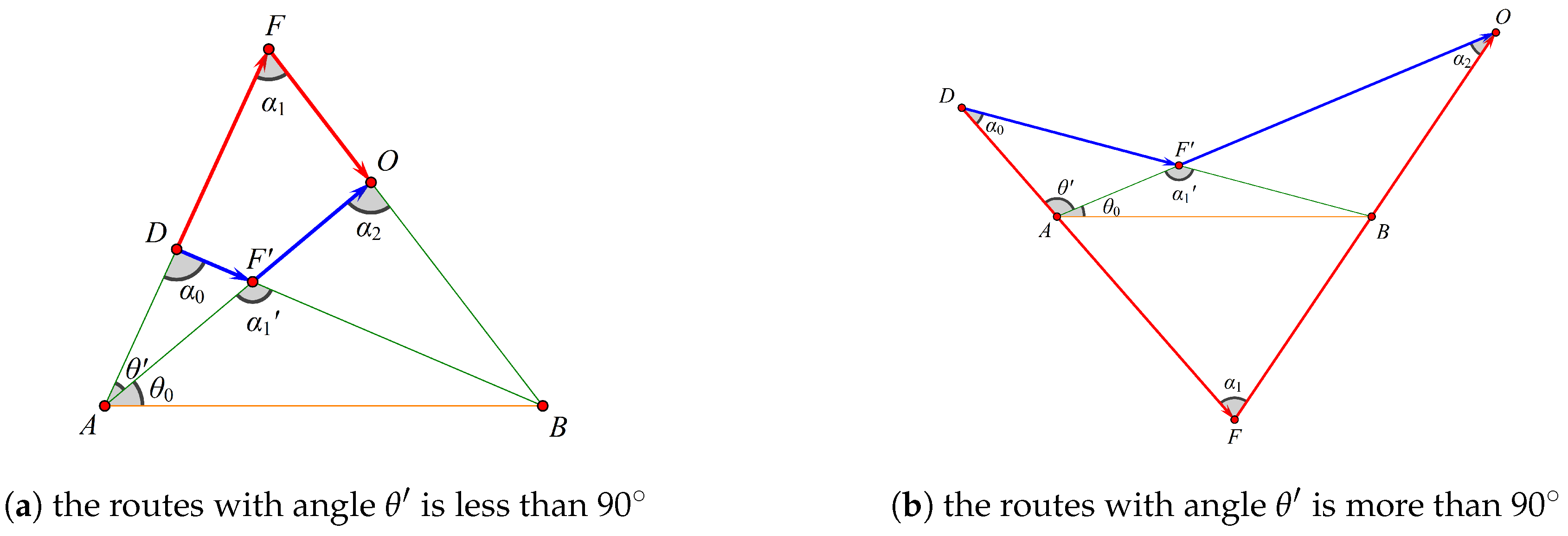
2.2. Two-Step Adjustment Strategy

After the receiving UAV has completed its positioning, it needs to be adjusted to the target position O. Compared with the positioning scheme, this adjustment scheme requires only two transmitting UAVs and one receiving UAV to complete the measurement of an angle.
A. Mathematical Model
In this model, the Cartesian coordinate system is established with point A as the origin and the direction from A to B as the positive direction of the polar coordinate system. Since the polar coordinates of the localized UAV at point D are ρ , θ 0 + θ , by observing the initial position of the receiving UAV, a two-step adjustment strategy can be used according to the initial movement direction of the receiving UAV. As shown in Figure 5, the trajectories of the two routes are indicated by red and blue arrows at different positional situations, respectively.
Model I: The receiving UAV starts its first movement along the straight line, passing through points A and D , in either the direction of AD or DA .
In that case, the point F is the stopping position of the receiving UAV after the first movement, and the coordinates of F are set to ( ρ F , θ 0 + θ ) , which are the coordinates after localization using Equation (10). The point O is the stopping point of the receiving UAV after the second movement and is the target point of the receiving UAV. When the azimuth information received by the receiving UAV is α 1 , it will stop its first movement and start its second movement along the straight line passing through points O and B, in either the direction of O B or B O . When the azimuth information received by the receiving UAV is α 2 , it will stop its second movement.
Step 1: In A F B , from α 2 and θ , we can obtain α 1 = α 2 θ . According to the sine theorem of the triangle, we can further obtain the representation as:
A F sin A O F = A O sin A F O .
Since A O = ρ 0 , A F = ρ F , sin A F O = sin α 1 , sin A O F = sin α 1 + θ , that is,
ρ F = sin α 1 + θ sin α 1 ρ 0 .
The distance S 1 of the first movement of the receiving UAV is A F A D . The coefficient that determines the direction of the first movement of the receiving UAV is δ 1 , which is δ 1 = A F A D D F . From Figure 6, it can be obtained that: when δ 1 is 1, the receiving UAV moves in the direction away from UAV A. When δ 1 is −1, the receiving UAV moves in the direction of the approaching UAV A. Further, by combining Equations (3) and (5), the distance S 1 of the first movement can be represented as:
S 1 = δ 1 D F , = ρ F ρ .
Step 2: The distance S 2 of the second movement of the receiving UAV is F O . The length of F O obtained from F ρ F , θ 0 + θ and O ρ 0 , θ 0 , that is:
F O = ρ F 2 + ρ 0 2 2 ρ F ρ 0 cos θ .
The coefficient that determines the direction of the second movement of the UAV D is δ 2 , which is δ 2 = B O F B O F . Since B O = ρ B 2 + ρ 0 2 2 ρ B ρ 0 cos θ 0 , F B = ρ B 2 + ρ F 2 2 ρ B ρ F cos ( θ 0 + θ ) . From Figure 6, it can be obtained that: when δ 2 is 1, UAV D moves in the direction away from the UAV at point B. When δ 1 is −1, the receiving UAV moves in the direction of the approaching UAV at point B. Further, by combining Equations (7) and (8), the distance S 2 of the second movement can be represented as:
S 2 = δ 2 O F , = ρ B 2 + ρ 0 2 2 ρ B ρ 0 cos θ 0 ρ B 2 + ρ F 2 2 ρ B ρ F cos θ 0 + θ .
In summary, the receiving UAV starts its first movement along the straight line passing through points A and D. It moves in the direction away from the UAV A when δ 1 = 1 , S 1 > 0 , or it moves in the direction of approaching the UAV at point A when δ 1 = 1 , S 1 < 0 . The receiving UAV stops moving when the azimuth information it receives is α 1 = α 2 θ . At the same time, the receiving UAV has reached point F and completed the first movement, whose distance is S 1 . The receiving UAV starts its second movement along the straight line passing through points O and B. It moves in the direction away from the UAV at point B when δ 2 = 1 , S 2 > 0 , or it moves in the direction of approaching the UAV at point A when δ 2 = 1 , S 2 < 0 . The receiving UAV stops moving when the azimuth information it receives is α 2 . At the same time, the receiving UAV has reached the target point O and completed its second movement, whose distance is S 2 . The Model I can be represented as:
α 1 = α 2 θ , ρ F = sin α 1 + θ sin α 1 ρ 0 , S 1 = ρ F ρ , S 2 = ρ B 2 + ρ 0 2 2 ρ B ρ 0 cos θ 0 ρ B 2 + ρ F 2 2 ρ B ρ F cos θ 0 + θ .
Model II: The receiving UAV starts its first movement along the straight line passing through points D and B in either the direction of DB or BD .
Step 1: In A F B , from α 2 and θ , according to the sine theorem of the triangle, we can further obtain the representation as:
A B sin A F B = A F sin A B F .
Since A B = ρ B , A F = ρ F , sin A F B = sin α 1 , sin A B F = sin α + θ 0 . So, ρ F = sin α 1 + θ 0 sin α 1 ρ B . The distance S 1 of the first movement of the receiving UAV is D F . The length of D F obtained from F ρ F , θ 0 and D ρ , θ 0 + θ , that is:
D F = ρ F 2 + ρ 2 2 ρ F ρ cos θ .
The coefficient that determines the direction of the first movement of the UAV is δ 1 , which is δ 1 = F B D B D F . Since F B = ρ F 2 + ρ B 2 2 ρ F ρ B cos θ 0 , D B = ρ 2 + ρ B 2 2 ρ ρ B cos ( θ 0 + θ ) . From Figure 7, it can be obtained that: when δ 1 is 1, the receiving UAV moves in the direction away from point B. When δ 1 is −1, the receiving UAV moves in the direction of approaching UAV at point B. Further, by combining δ 1 in Equations (13) and (14), the distance S 1 of the first movement can be represented as:
S 1 = δ 1 D F , = ρ F 2 + ρ B 2 2 ρ F ρ B cos θ 0 ρ 2 + ρ B 2 2 ρ ρ B cos θ 0 + θ .
Step 2: The distance S 2 of the second movement of the receiving UAV is F O . The length of F O obtained from F ( ρ F θ 0 ) and O ( ρ 0 , θ 0 ) , that is:
F O = ρ 0 ρ F .
The coefficient that determines the direction of the second movement of the receiving UAV is δ 2 , which is δ 2 = A O A F F O . From Figure 6, it can be obtained that: when δ 2 is 1, the receiving UAV moves in the direction away from the UAV A. When δ 2 is −1, the receiving UAV moves in the direction of approaching the UAV at point A. Further, by combining Equations (16) and (20), the distance of the second movement can be represented as:
S 2 = δ 2 F O , = ρ ρ F .
In summary, the receiving UAV starts its first movement along the straight line passing through points B and D. It moves in the direction away from the UAV B when δ 1 = 1 , S 1 > 0 , or it moves in the direction of approaching the UAV at point B when δ 1 = 1 , S 1 < 0 . The receiving UAV stops moving when the azimuth information it receives is α 1 = α 0 + θ . At the same time, the receiving UAV has reached the point F and completed its first movement, whose distance is S 1 . The receiving UAV starts its second movement along the straight line passing through points O and A. It moves in the direction away from the UAV at point A when δ 2 = 1 , S 2 > 0 , or it moves in the direction of approaching the UAV at point A when δ 2 = 1 , S 2 < 0 . The receiving UAV stops moving when the azimuth information it receives is α 2 . At the same time, the receiving UAV has reached the target point O and completed its second movement, whose distance is S 2 . The Model II can be represented as:
α 1 = α 0 + θ , ρ F = sin α 1 + θ 0 sin α 1 ρ B , S 1 = ρ F 2 + ρ B 2 2 ρ F ρ B cos θ 0 ρ 2 + ρ B 2 2 ρ ρ B cos θ 0 + θ , S 2 = ρ ρ F .
B. Two Step Adjustment Strategy.
The above shows two ways in which the receiving UAV can be positioned by two transmitting UAVs to reach the target location after a two-step movement. Therefore, one of these two options can be chosen to complete the adjustment. In order to minimize the UAV movement distance and reduce the UAV movement energy cost, the option with the shorter overall movement distance of these two options needs to be selected. When the total distance of the first movement is R I and the total distance of the second movement is R II , then the shorter path R can be represented as:
R I = S 1 + S 2 , R II = S 1 + S 2 , R = min R I , R II .
The concrete implementation of the two-step adjustment strategy is shown in Algorithm 1.
Algorithm 1: Two step adjustment strategy.
    Input: The coordinate of the receiving UAV, the coordinates of positioning UAVs, and the coordinate of the target location, constant θ , ε = 1 × 10 6 .
    Output: Move the receiving UAV to the coordinate of the target location.
Drones 08 00243 i001

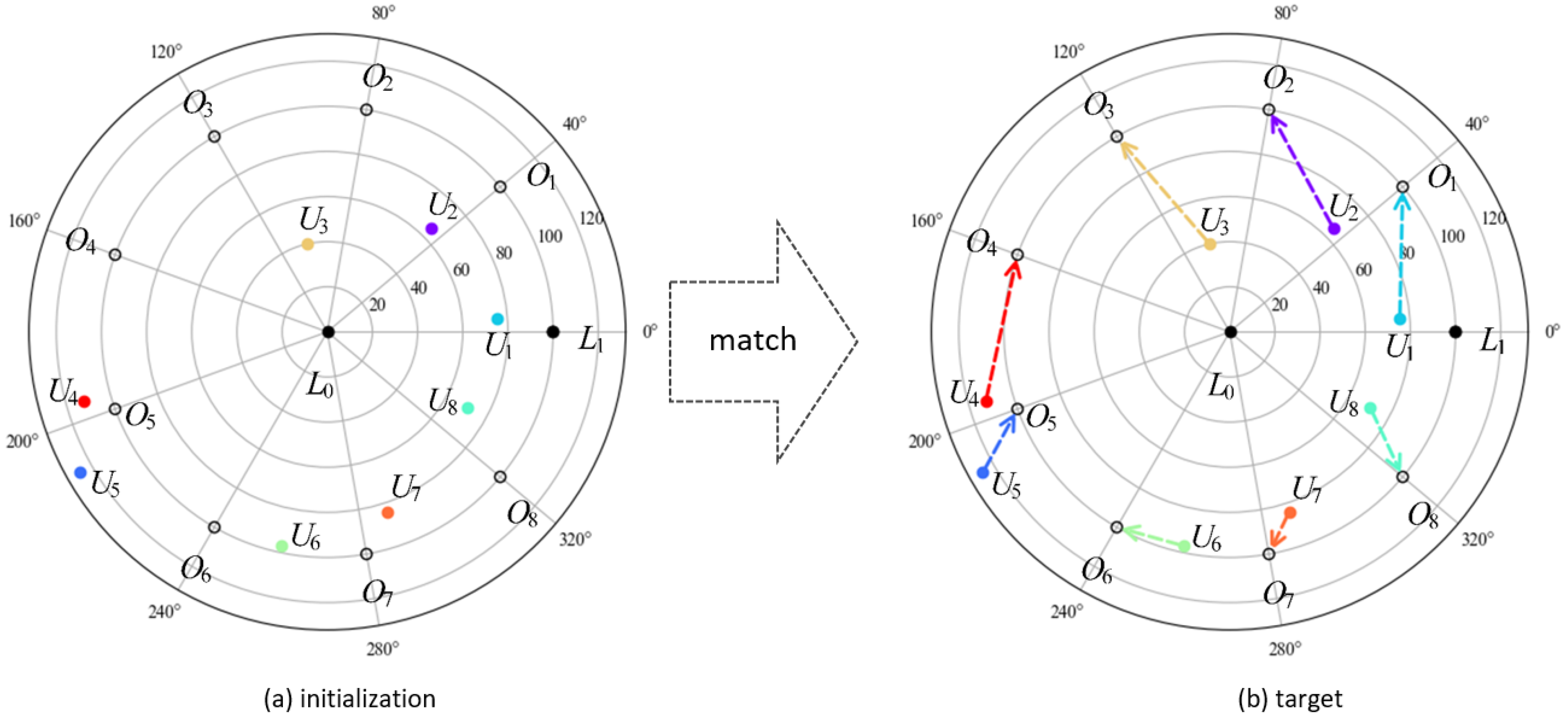
2.3. UAV Swarm Formation Scheme

After determining the movement strategy of a single UAV, it is also necessary to consider the movement strategy of the whole UAV swarm. In order to make the UAV swarm formation flight with the least overall energy consumption and the shortest movement distance, we introduce the Hungarian algorithm to assign the optimal matching scheme for all UAVs.
Figure 8 shows an example of an assigned task with eight receiving UAVs, denoted by U i ( i 1 , 2 , , 8 ), and eight target positions, denoted by O i ( i 1 , 2 , , 8 ). Figure 8a shows the initial positions and target positions of the eight UAVs, and Figure 8b shows a scheme of the matching problem. There are two initial transmitting UAVs, L 0 and L 1 , and a polar coordinate system is established with the coordinate of the UAV L 0 as the origin and the direction from L 0 to L 1 as the positive direction of the polar coordinate system. The distance between L 0 and L 1 is r ( r = 100 ). UAV L 1 is used to assist in localizing the position of the first UAV. After U i has reached its target O i , U i becomes U i and adjusts UAV U i + 1 with L 0 to reach O i + 1 . These steps are repeated until all receiving UAVs are adjusted.
In order to obtain the shortest distance for the overall movement of the UAV, we first calculate the distance matrix n×n from the coordinates of each receiving UAV to the target coordinates. Since each target location corresponds to a fixed transmitter UAV (e.g., the target location O i + 1 corresponds to the origin and O i transmitter UAV locations). Therefore, the distance of any receiving UAV to reach any target location can be obtained by the two-step adjustment strategy. The optimal matching scheme can then be determined using the Hungarian algorithm. So, the concrete implementation of the formation adjustment scheme of UAVs is shown in Algorithm 2.
Algorithm 2: The formation scheme of UAVs.
   Input: The initialization coordinates of n UAVs and the coordinate of n target coordinates.
   Output: The best formation scheme.
1 Calculate the n × n matrix between the initialization coordinates of n UAVs and the coordinate of n target coordinates with Equation (24).
2 Hungarian algorithm is used for target location assignment.
3 Output the best match 1 × n matrix;
4 Use the matching matrix as the adjustment scheme for the UAVs;

3. Experiments

In this section, we validate our proposed UAV swarm formation flight method based on pure azimuth passive positioning. The experiments evaluate the accuracy of the two-circle positioning model and the efficiency of the two-step adjustment strategy across different scales, involving 8 and 20 UAVs. The results demonstrate that our method significantly reduces the total movement length (measured in units) required for UAVs to reach their target positions compared to the geometric optimization strategy, while also offering lower computational complexity. The high positioning accuracy and effective position assignment are demonstrated through detailed visualizations of UAV movement paths and comparisons with other adjustment strategies. These findings confirm the practical applicability and advantages of our method for real-time, large-scale UAV swarm formations. Note that all lengths are measured in units, and all angles are measured in degrees.

3.1. Experiment Setting

In experiments, we used Python 3.9.18 for data processing and algorithm implementation, MATLAB 2022b for numerical simulation and visualization, and Sketchpad 5.06 for graphical representations. These tools are run on the Windows 10 platform.

3.2. The Validity of the Two-Circle Positioning Model

In order to demonstrate the effectiveness of the two-circle positioning model, we first fix the coordinates of the three transmitting UAVs and the target point with the following parameters: ρ 0 = 5.30 units, ρ B = 9.55 units, ρ C = 6.13 units, θ 0 = 30.91°, and θ C = 71.64°. Next, we analyze the error of the two-circle positioning model under different scenarios by varying the relative position of the UAV receiving the signal. In the coordinate system with O as the origin and A O as the polar axis, the receiving angles α ( A D B ) and β ( A D C ) are used in the calculation of the localization model in Equations (10) and (11), respectively, and the localization coordinates of the receiving UAV are obtained as r , θ . We use the error radius r e to measure the fitting error of the two-circle positioning model, which geometrically represents the Euclidean distance between the estimated positions and target positions in polar coordinates. The error radius r e is calculated using the formula:
r e = r 2 + r target 2 2 r r target cos ( θ θ target )
where r and θ are the estimated position’s radial distance and angle, and r target and θ target are the target position’s radial distance and angle. Smaller values of the error radius indicate a more accurate fit.
In details, we chose seven representative situations in our experiment, notated as ‘Inside’, ‘Left’, ‘Right’, ‘Down’, ‘Top left’, ‘Bottom left’, and ‘Bottom right’. ‘Inside’ represents the case where the coordinates of the receiving UAV are inside the triangle A B C . ‘Left’, ‘Right’, and ‘Down’ represent the cases where the coordinates of the UAV D are over the three sides outside the triangle A B C , respectively. ‘Top left’, ‘Bottom left’, and ‘Bottom right’ represent the cases where the coordinates of the receiving UAV is above the three top corners outside the triangle A B C . The different locations of the receiving UAV used for testing are shown in Figure 9, and the test results are shown in Table 2. It can be observed that the positioning coordinates of the receiving UAV are very close to the actual coordinates, indicating the high accuracy of this positioning system.

3.3. Compared to the Representative Adjustment Strategy

To validate the effectiveness of the proposed two-step strategy for UAV swarm formation adjustment, we compare it with a geometric optimization-based approach ([7]). This approach stems from classical geometry problems and adjusts the UAV position by measuring and optimizing the path angle error through iterative calculations. This method requires iterative calculations to find the optimal path. Specifically, the geometric optimization method determines paths by calculating multiple angles between initial positions and target positions. Then, it minimizes the squared sum of angle errors by adjusting the UAV paths iteratively. In this process, the geometric optimization method uses gradient descent to determine the optimization direction. By calculating the gradient of the objective function and moving in the opposite direction, the error is continually reduced. We also compare three different two-step adjustment strategies.
Since both the comparison method and the proposed method use the Hungarian algorithm, we can use the total length of the UAV’s movement to measure the performance of the different adjustment strategies. We conducted experiments on 8 UAVs and 20 UAVs in the formation scheme, respectively. As shown in Table 3 and Table 4, the experimental results demonstrate the formation effect with different numbers of UAVs. The movement distance of each UAV and the total length of the formation are also provided in this analysis.
As shown in Table 3, given the same initialized and target positions of the UAVs, the total path length for the geometric optimization strategy is 753.47 units, while the proposed two-step strategy achieves 491.58 units. The total length adjusted by our method is only 65.24% of that of the comparison method. Similarly, as shown in Table 4, in the 20 UAVs formation, the total length of movement for the comparison strategy is 1859.19, while the two-step adjustment strategy proposed requires 830.38, which is only 44.66% of its total length. Meanwhile, by comparing the individual path lengths of the 20 UAVs, it can also be found that most of the paths of the proposed two-step strategy are smaller than the length of the comparison strategy. For example, UAV U 1 moves a total of 74.15 units in the proposed two-step strategy, whereas it moves 339.04 units using the geometric optimization strategy. Similarly, UAV U 6 requires 45.34 units of movement under the proposed two-step strategy, compared to 133.09 units using the geometric optimization strategy. And a small number of paths have slightly larger path lengths than the comparison strategy, but the difference is not significant. The results show that the proposed two-step adjustment strategy requires less cost in UAV swarm formations, making it more suitable for large-scale UAV formations with stringent real-time requirements and demonstrating its practical advantages in terms of passive UAV localization and fast formation adjustment.
As shown in Table 5, we further compare the two adjustment strategies in terms of three aspects: total move length, time complexity, and optimization method. We can see that, compared to the comparison strategy, the proposed two-step strategy outperforms the comparison method in three aspects. In details, the total path length for this method is 753.47 units, but it requires multiple iterations of angle error calculations, making its overall computational complexity high. The time complexity of the geometric optimization method is O ( k · n ) , where k is the number of iterations and the average is greater than 12, and the number of times increases gradually with the increase of the polar radius. n is the number of UAVs. In contrast, the two-step method simplifies the path planning process by requiring only one angle measurement and two liner movements with Equation (24), significantly reducing computational complexity, with a total path length of 491.58 units. The time complexity of the two-step method is lower, at O ( n ) , where n is the number of UAVs. This makes the two-step method more suitable for large-scale UAV formation adjustments with high real-time requirements (e.g., 20, 50, or even more). Its scalability makes the two-step adjustment strategy highly versatile and adaptable to various operational requirements, ensuring efficient and real-time adjustments in UAV swarm formations regardless of their scale.
As shown in Figure 10c,d, we show the visualization of the movement paths for both adjustment strategies. The proposed two-step adjustment strategy needs to move along two directions and does not require iterative optimization in a comprehensive perspective. The strategy is easier to operate and has better robustness. Therefore, the two-step strategy has significant advantages in practical applications of passive positioning of UAVs, making it suitable for scenarios that require rapid formation adjustments.

3.4. Compared to Different Two-Step Adjustment Strategy

To further validate the effectiveness of the proposed two-step adjustment strategy for the formation of eight UAVs, the moving distances of different two-step adjustment strategies are compared and analyzed in this section. In part B of Section 2.1, we put forward two adjustment strategies, Model I and Model II, through the two-circle positioning model. Here, we compare the distance costs of these two two-step adjustment strategies. As shown in Table 6, each column shows the distance traveled by each UAV under different movement strategies. The move length S 1 of the first step and the move length S 2 of the second step are shown in parentheses. It can be observed that when the initialized coordinates of the UAVs and the target coordinates of the UAVs are the same, the total path length of Model I is 616.5 units, the total path length of Model II is 571.27 units, and the proposed two-step strategy achieves 491.58 units. Compared to Model I strategy and Model II strategy, the proposed two-step adjustment strategy can choose the shortest path scheme of their two strategies, thus reducing the total length of the UAV adjustment. As shown in Figure 10a,b, we also show the visualization of the movement paths for both Model I and Model II. It can be seen that the proposed two-step strategy has a distinct advantage over the comparison strategy (Figure 10c).

4. Discussion

For the UAV swarm formation, we mainly focus on the positioning and adjustment aspects and propose a 2D two-circle positioning model based on angle information and a two-step adjustment strategy. The superiority of the proposed method is demonstrated in UAV swarm formation experiments at different scales. However, in order to focus more on localization and adjustment aspects, we do not consider the influence of the channel model on the positioning model as well as the derivation and validation of the positioning model for the 3D coordinate system, which are the directions for further research in our future work.

5. Conclusions

In this paper, we propose a new solution for UAV positioning, adjustment, and swarm formation based on pure azimuth passive positioning. In particular, we propose the two-circle positioning model based on angle information, which requires only three transmitter UAVs with known coordinates to perform pure azimuth passive localization of a receiver UAV with an unknown position. Further, we design a two-step adjustment strategy that enables the receiving UAV to reach the target position through a two-step movement. Based on this, we construct an efficient UAV swarm formation scheme. The scheme obtains the optimal target matching paths of the UAV swarm through the Hungarian algorithm, which further improves the execution efficiency of the scheme. Simulation results at different scales show that the proposed scheme significantly reduces the total flight distance and energy consumption of the UAV swarm.

Author Contributions

Conceptualization, Z.K., Y.D. and H.Y.; methodology, Z.K., Y.D. and H.Y.; software, Y.D.; validation, Z.K., Y.D. and H.Y.; formal analysis, Y.D., H.Y. and L.Y.; investigation, L.Y.; resources, Z.K., S.Z. and B.L.; data curation, L.Y.; writing—original draft preparation, Y.D., H.Y., L.Y. and Z.K.; writing—review and editing, Z.K., Y.D. and B.L.; visualization, Y.D. and Z.K.; supervision, Z.K.; project administration, Z.K.; funding acquisition, Z.K., S.Z. and B.L. All authors have read and agreed to the published version of the manuscript.

Funding

This research was funded by Natural Science Foundation of Hubei Province of China, grant number 2023AFB351; and the University-Industry Collaborative Education Program, grant number 230705841293521.

Data Availability Statement

Data are self-contained within this article.

Conflicts of Interest

The authors declare no conflicts of interest.

References

  1. Li, B.; Song, C.; Bai, S.; Huang, J.; Ma, R.; Wan, K.; Neretin, E. Multi-UAV Trajectory Planning during Cooperative Tracking Based on a Fusion Algorithm Integrating MPC and Standoff. Drones 2023, 7, 196. [Google Scholar] [CrossRef]
  2. No, T.S.; Kim, Y.; Tahk, M.-J.; Jeon, G.-E. Cascade-Type Guidance Law Design for Multiple-UAV Formation Keeping. Aerosp. Sci. Technol. 2011, 15, 431–439. [Google Scholar] [CrossRef]
  3. Hao, L.; Xiangyu, F.; Manhong, S. Research on the Cooperative Passive Location of Moving Targets Based on Improved Particle Swarm Optimization. Drones 2023, 7, 264. [Google Scholar] [CrossRef]
  4. Zhu, S. Research on Multi-UAV Cooperative Path Planning for Target Positioning and Tracking. Master’s Thesis, Xidian University, Xi’an, China, 2021. [Google Scholar]
  5. Adoni, W.Y.H.; Lorenz, S.; Fareedh, J.S.; Gloaguen, R.; Bussmann, M. Investigation of Autonomous Multi-UAV Systems for Target Detection in Distributed Environment: Current Developments and Open Challenges. Drones 2023, 7, 263. [Google Scholar] [CrossRef]
  6. Liao, J.; Bang, H. Transition Nonlinear Blended Aerodynamic Modeling and Anti-Harmonic Disturbance Robust Control of Fixed-Wing Tiltrotor UAV. Drones 2023, 7, 255. [Google Scholar] [CrossRef]
  7. Yang, Y.; Xiong, X.; Yan, Y. UAV Formation Trajectory Planning Algorithms: A Review. Drones 2023, 7, 62. [Google Scholar] [CrossRef]
  8. Yuan, G.; Duan, H. Robust Control for UAV Close Formation Using LADRC via Sine-Powered Pigeon-Inspired Optimization. Drones 2023, 7, 238. [Google Scholar] [CrossRef]
  9. Yue, J.; Qin, K.; Shi, M.; Jiang, B.; Li, W.; Shi, L. Event-Trigger-Based Finite-Time Privacy-Preserving Formation Control for Multi-UAV System. Drones 2023, 7, 235. [Google Scholar] [CrossRef]
  10. Zhu, L.; Ma, C.; Li, J.; Lu, Y.; Yang, Q. Connectivity-Maintenance UAV Formation Control in Complex Environment. Drones 2023, 7, 229. [Google Scholar] [CrossRef]
  11. Wang, L. Multi-Target Localization Based on Convolutional Neural Networks. Master’s Thesis, Chang’an University, Xi’an, China, 2019. [Google Scholar]
  12. Tong, P.; Yang, X.; Yang, Y.; Liu, W.; Wu, P. Multi-UAV Collaborative Absolute Vision Positioning and Navigation: A Survey and Discussion. Drones 2023, 7, 261. [Google Scholar] [CrossRef]
  13. Ren, Y. A Study of Multi-Satellite Passive Location System Based on TDOA. Master’s Thesis, Xidian University, Xi’an, China, 2021. [Google Scholar]
  14. Yin, J.; Wan, Q.; Yang, S.; Ho, K.C. A Simple and Accurate TDOA-AOA Localization Method Using Two Stations. IEEE Signal Process. Lett. 2016, 23, 144–148. [Google Scholar] [CrossRef]
  15. Wang, M. Research on Multi-Station Passive Location and Tracking Algorithm Based on TDOA/AOA. Master’s Thesis, Harbin Engineering University, Harbin, China, 2019. [Google Scholar]
  16. Song, Y. Research on Ultra-Wideband Indoor Positioning Technology. Master’s Thesis, Xi’an University of Science and Technology, Xi’an, China, 2019. [Google Scholar]
  17. Wang, B.; Wang, G.; He, Y. Progress of Research on Multi-Sensor Bearing-Only Passive Locating Algorithm. Electron. Opt. Control 2012, 19, 56–62. [Google Scholar]
  18. Sun, H. Research on the Algorithm of Passive Location with Bearing-Only Measurement. Master’s Thesis, Harbin Engineering University, Harbin, China, 2010. [Google Scholar]
  19. Mao, K.; Yan, Z.; Han, C.; Zhang, Y. A UAV-Aided Real-Time Channel Sounder for Highly Dynamic Nonstationary A2G Scenarios. IEEE Trans. Instrum. Meas. 2023, 72, 6504515. [Google Scholar] [CrossRef]
  20. Lyu, Y.; Sun, W.; He, R.; Ai, B.; Guan, K. Low-Altitude UAV Air-to-Ground Multilink Channel Modeling and Analysis at 2.4 and 5.9 GHz. IEEE Antennas Wirel. Propag. Lett. 2023, 22, 2135–2139. [Google Scholar] [CrossRef]
  21. Xu, H.; Zhang, Y.; Ba, B.; Wang, D.; Li, X. Fast Joint Estimation of Time of Arrival and Angle of Arrival in Complex Multipath Environment Using OFDM. IEEE Access 2018, 6, 60613–60621. [Google Scholar] [CrossRef]
  22. Wu, Z.; Du, M.; Bi, D.; Pan, J. IRelNet: An Improved Relation Network for Few-Shot Radar Emitter Identification. Drones 2023, 7, 312. [Google Scholar] [CrossRef]
  23. Hernandez, M.; Farina, A. PCRB and IMM for Target Tracking in the Presence of Specular Multipath. IEEE Trans. Aerosp. Electron. Syst. 2020, 56, 2437–2449. [Google Scholar] [CrossRef]
  24. Li, S.; Li, Y.; Zhu, J.; Liu, B. Predefined Location Formation: Keeping Control for UAV Clusters Based on Monte Carlo Strategy. Drones 2022, 7, 29. [Google Scholar] [CrossRef]
  25. Fu, T.; Ding, G.; Tian, W.; Yang, Y. Research on UAV Formation Positioning and Adjustment Strategy Based on Analytic Geometry. J. Xi’an Univ. Technol. 2023, 39, 79–88. [Google Scholar] [CrossRef]
  26. Wu, E.; Sun, Y.; Huang, J.; Zhang, C.; Li, Z. Multi UAV Cluster Control Method Based on Virtual Core in Improved Artificial Potential Field. IEEE Access 2020, 8, 131647–131661. [Google Scholar] [CrossRef]
  27. Liu, Y.; Bucknall, R. A Survey of Formation Control and Motion Planning of Multiple Unmanned Vehicles. Robotica 2018, 36, 1019–1047. [Google Scholar] [CrossRef]
  28. Zhang, Z.; Lu, H.; Ma, Y.; Ban, X.; Zhang, J. Multi-aircraft Cooperative Passive Location Optimization Algorithm Based on AOA Model. In Proceedings of the 40th Chinese Control Conference (CCC), Shanghai, China, 26–28 July 2021; Technical Committee on Control Theory, Chinese Association of Automation, Chinese Association of Automation, and Systems Engineering Society of China. Volume 15, pp. 559–564. [Google Scholar]
  29. Li, B.; Zhao, K.; Shen, X. Dilution of Precision in Positioning Systems Using Both Angle of Arrival and Time of Arrival Measurements. IEEE Access 2020, 8, 192506–192516. [Google Scholar] [CrossRef]
  30. Cheung, K.-M.; Lee, C. A New Geometric Trilateration Scheme for GPS-Style Localization. The Interplanetary Network Progress Report. 2017, 42–209. Available online: https://ipnpr.jpl.nasa.gov/progress_report/42-209/title.htm (accessed on 15 April 2024).
Figure 1. Three key aspects of the proposed UAV swarm formation method.
Drones 08 00243 g001
Figure 2. Example of using three transmitting UAVs and the receiving UAV to obtain angle information for passive positioning.
Drones 08 00243 g002
Figure 3. Comparison of different positioning principle.
Drones 08 00243 g003
Figure 4. Comparison of different positioning principle.
Drones 08 00243 g004
Figure 5. The two adjustment routes for the UAV in different positional situations.
Drones 08 00243 g005
Figure 6. The route for Model I in different positional situations.
Drones 08 00243 g006
Figure 7. The route for Model II in different positional situations.
Drones 08 00243 g007
Figure 8. An example of an assigned task of eight receiving UAVs.
Drones 08 00243 g008
Figure 9. Examples of different spatial positions of the receiving UAV D and triangle A B C .
Drones 08 00243 g009
Figure 10. Visualization of movement paths for different adjustment strategies.
Drones 08 00243 g010
Table 1. Symbols and descriptions in new UAV swarm formation flight method.
SymbolDescription
A , B , C The points of the transmitting UAVs
DThe point of the receiving UAV
ρ Radial distance of the receiving UAV at point D
ρ 0 Radial distance of the target point O
ρ B Radial distance of the transmitting UAV at point B
ρ C Radial distance of the transmitting UAV at point C
θ 0 Angle O A B formed by points O, A and B
θ Angle D A O formed by points A, D, and O
θ C Polar angle coordinate of transmitting UAV at point C
rDistance between the target point O and the receiving UAV at point D
θ Angle formed between vector A O and vector O D
α Angle A D B formed by points A, D, and B
β Angle A D C formed by points A, D, and C
α Angle A D B formed by points A, D , and B
β Angle A D C formed by points A, D , and C
OOrigin of the polar coordinate system at the target point
α 1 Intermediate target angle calculated in the first step of Model I
α 2 Intermediate target angle calculated in the second step of Model I
S 1 The distance movement of the first step in Model I
S 2 The distance movement of the second step in Model I
δ 1 Coefficient determining the direction of the first movement
ρ F Radial distance of the stopping position after the first movement in Model I
α 1 Intermediate target angle calculated during the first step of Model II
α 2 Intermediate target angle calculated in the second step of Model II
S 1 The distance movement of the first step in Model II
S 2 The distance movement of the second step in Model II
δ 2 Coefficient determining the direction of the second movement
ρ F Radial distance of the intermediate point F in Model II
R I Total distance of the first adjustment route
R II Total distance of the second adjustment route
RThe shorter total distance between R I and R II
U i The i-th receiving UAV
O i The i-th target position
L 0 The initial transmitting UAV used as the origin of the polar coordinate system
L 1 The initial transmitting UAV used to assist in localizing the position of the first UAV
rThe radius of the polar coordinate system, set to 100
n × n matrixThe distance matrix from the coordinates of each receiving UAV to the target coordinates
Table 2. The error radius of positioning model of the receiving UAV at different spatial positions.
Position Coord.Target Coord.Error Radius (Units)
Inside(1.77, 135.26°)(1.7690, 135.1851°)0.0025
Left(6.62, 132.61°)(6.6181, 132.5999°)0.0022
Right(8.38, 16.66°)(8.3792, 16.6902°)0.0045
Down(5.51, −132.28°)(5.5065, −132.2874°)0.0036
Top left(6.72, 89.59°)(6.7238, 89.5719°)0.0044
Bottom left(8.49, −174.11°)(8.4842, −174.1090°)0.0058
Bottom right(9.05, −61.30°)(9.0446, −61.2753°)0.0067
Table 3. The move length of different adjustment strategies on 8-UAV cluster initialization coordinates (Init Coord.) and target coordinates (Target Coord.) in polar coordinates.
No.Init Coord.Target Coord.Geometric OptimizationTwo-Step Strategy
U 1 (75.58, 4.66°)(100.00, 40.00°)261.6481.84
U 2 (64.99, 45.21°)(100.00, 80.00°)33.2691.21
U 3 (40.36, 103.13°)(100.00, 120.00°)139.0682.81
U 4 (112.35, 195.95°)(100.00, 160.00°)51.6682.67
U 5 (125.84, 209.70°)(100.00, 200.00°)33.9336.52
U 6 (97.02, 257.83°)(100.00, 240.00°)125.1745.34
U 7 (84.11, 288.20°)(100.00, 280.00°)22.2429.84
U 8 (70.59, 331.74°)(100.00, 320.00°)86.5143.95
Total--753.47491.58
Table 4. The move length of the different adjustment strategy on 20-UAV cluster initialization coordinates (Init Coord.), target coordinates (Target Coord.) in polar coordinates.
No.Init Coord.Target Coord.Geometric OptimizationTwo-Step Strategy
U 1 (63.22, 356.41°)(100.00, 17.14°)339.0474.15
U 2 (63.40, 50.45°)(100.00, 34.29°)44.0248.03
U 3 (106.70, 47.58°)(100.00, 51.43°)57.8414.22
U 4 (76.07, 61.12°)(100.00, 68.57°)94.7235.80
U 5 (91.13, 77.02°)(100.00, 85.71°)87.3422.87
U 6 (81.75, 87.07°)(100.00, 102.86°)133.0945.34
U 7 (55.46, 130.98°)(100.00, 120.00°)60.1749.85
U 8 (142.39, 134.34°)(100.00, 137.14°)98.1647.91
U 9 (89.99, 146.39°)(100.00, 154.29°)89.3422.63
U 10 (81.91, 173.37°)(100.00, 171.43°)79.9819.97
U 11 (142.84, 194.59°)(100.00, 188.57°)103.1848.06
U 12 (149.85, 217.47°)(100.00, 205.71°)88.8360.79
U 13 (91.18, 217.10°)(100.00, 222.86°)113.5117.86
U 14 (138.36, 225.17°)(100.00, 240.00°)92.1264.63
U 15 (139.80, 250.65°)(100.00, 257.14°)101.8152.17
U 16 (136.23, 270.87°)(100.00, 274.29°)84.2842.92
U 17 (100.84, 305.10°)(100.00, 291.43°)19.6826.96
U 18 (147.51, 336.24°)(100.00, 308.57°)93.3278.87
U 19 (75.07, 344.66°)(100.00, 325.71°)42.4044.67
U 20 (103.08, 349.62°)(100.00, 342.86°)36.3612.68
Total--1859.19830.38
Table 5. Comparison of geometric optimization strategy and two-step adjustment strategy.
Geometric OptimizationTwo-Step Strategy
Total length753.47491.58
Complexity O ( k · n ) O ( n )
OptimizationGradient descentEquation (24)
Table 6. The moving length of the receiving UAV using different two-step strategies in formation schemes. Where the move length S 1 of the first step and the move length S 2 of the second step are shown in parentheses.
No.Model IModel IITwo-Step Strategy
U 1 81.84 (21.86, 59.98)124.19 (54.05, 70.14)81.84 (21.86, 59.98)
U 2 91.21 (32.20, 59.01)127.07 (48.77, 78.30)91.21 (32.20, 59.01)
U 3 82.81 (53.75, 29.06)84.29 (14.45, 69.84)82.81 (53.75, 29.06)
U 4 160.33 (55.48, 104.85)82.67 (66.36, 16.31)82.67 (66.36, 16.31)
U 5 37.06 (17.66, 19.40)36.52 (24.25, 12.27)36.52 (24.25, 12.27)
U 6 60.72 (21.95, 38.77)42.74 (30.12, 12.62)42.74 (30.12, 12.62)
U 7 38.70 (22.52, 16.18)29.84 (12.04, 17.80)29.84 (12.04, 17.80)
U 8 63.83 (39.90, 23.93)43.95 (14.43, 29.52)43.95 (14.43, 29.52)
Total616.50571.27491.58
Disclaimer/Publisher’s Note: The statements, opinions and data contained in all publications are solely those of the individual author(s) and contributor(s) and not of MDPI and/or the editor(s). MDPI and/or the editor(s) disclaim responsibility for any injury to people or property resulting from any ideas, methods, instructions or products referred to in the content.

