Article

Evaluation of Machine Learning Regression Techniques for Estimating Winter Wheat Biomass Using Biophysical, Biochemical, and UAV Multispectral Data

1
Department of Geography and Environment, The University of Western Ontario, London, ON N6G 3K7, Canada
2
The Institute for Earth and Space Exploration, The University of Western Ontario, London, ON N6A 3K7, Canada
*
Author to whom correspondence should be addressed.
Drones 2024, 8(7), 287; https://doi.org/10.3390/drones8070287
Submission received: 31 May 2024 / Revised: 22 June 2024 / Accepted: 23 June 2024 / Published: 26 June 2024
(This article belongs to the Special Issue Advances of UAV in Precision Agriculture)

Abstract

:
Crop above-ground biomass (AGB) estimation is a critical practice in precision agriculture (PA) and is vital for monitoring crop health and predicting yields. Accurate AGB estimation allows farmers to take timely actions to maximize yields within a given growth season. The objective of this study is to use unmanned aerial vehicle (UAV) multispectral imagery, along with derived vegetation indices (VI), plant height, leaf area index (LAI), and plant nutrient content ratios, to predict the dry AGB (g/m2) of a winter wheat field in southwestern Ontario, Canada. This study assessed the effectiveness of Random Forest (RF) and Support Vector Regression (SVR) models in predicting dry ABG from 42 variables. The RF models consistently outperformed the SVR models, with the top-performing RF model utilizing 20 selected variables based on their contribution to increasing node purity in the decision trees. This model achieved an R2 of 0.81 and a root mean square error (RMSE) of 149.95 g/m2. Notably, the variables in the top-performing model included a combination of MicaSense bands, VIs, nutrient content levels, nutrient content ratios, and plant height. This model significantly outperformed all other RF and SVR models in this study that relied solely on UAV multispectral data or plant leaf nutrient content. The insights gained from this model can enhance the estimation and management of wheat AGB, leading to more effective crop yield predictions and management.

1. Introduction

With the increasing growth of the global population, the strong demand for food sources and food security has highlighted the need to enhance the development of efficient and sustainable agricultural practices. In the modern era, challenges such as rising global food demand, crop diseases and pest outbreaks, limited cultivated areas, and climate change are affecting the entire agriculture industry. Tan and Reynolds found that in southern Ontario, water supply and demand are the major challenges for the agricultural industry [1]. Notably, farmers in the province are less concerned about climate change compared to those in regions where extreme weather events are more prevalent [2]. The agriculture and agri-food sectors contribute approximately 7% to Canada’s gross domestic product (GDP), and one in every nine jobs in Canada was provided by this sector in 2022 [3]. Although climate change is not an immediate challenge for the Canadian agricultural industry, it is prudent to be informed early and prepare for counteractions while we still have time to respond to unforeseen climate variations.
Precision agriculture (PA) utilizes advanced technologies and data analysis techniques to maximize crop output while minimizing inputs. This approach involves assessing quantified spatial and in situ plant data to guide agricultural practices, such as the application of water, labor, and fuel, thereby reducing costs and preventing excessive waste, like pesticide and nutrient loss. PA integrates various spatial technologies, including geographic information systems (GIS), handheld ground-based data collection devices, and remote sensing through ground-based or aerial vehicles, to develop and implement efficient agricultural strategies [4].
Above-ground biomass (AGB) is a frequently used parameter to indicate crop growth status and the effects of agricultural management practices, making AGB estimation one of the main applications in PA [5,6]. In this study, we adopt a multivariate approach to estimate AGB using biophysical and biochemical parameters, utilizing in situ field data and high-resolution multispectral imagery collected by an unmanned aerial vehicle (UAV). Biophysical parameters included plant height and the leaf area index (LAI). In the context of using plant height as a predictor of AGB, the literature includes UAV-based height extraction methods that provide comprehensive coverage of the studied field, with multispectral cameras and LiDAR systems being common approaches [6,7,8]. Research has yielded varying degrees of success in identifying plant height as an important factor correlating with AGB. Furthermore, the LAI has been proven to be a significant parameter for monitoring crop growth and estimating AGB. Liu et al. found a strong linear relationship between the LAI and AGB, though this relationship weakens after the crops’ senescence [9]. To explore the potential of variables that are strong predictors of AGB in the early growth stages of winter wheat, our study attempts to address the limitations of these variables in later growth stages by incorporating biochemical parameters.
While research related to biomass estimation is abundant, few studies have utilized biochemical parameters, such as plant nutrient contents, as predictors. Common variables in biomass and yield estimation included plant height, the LAI, and specific vegetation indices (VIs), like the renormalized difference vegetation index (RDVI) and the modified hyperspectral variant of the normalized difference vegetation index (NDVI-like) [7,10,11]. These variables measure the physical structures of plants and are indicative of plant biomass and yield, and it is well established that plant biochemistry is intricately linked to plant structure, health, and condition, all of which are critical factors in applying PA strategies [12]. According to Marschner (2001) [13], macronutrients, micronutrients, and beneficial elements are essential classes of nutrients that promote plant health and growth through various mechanisms. For instance, nitrogen is a crucial macronutrient and is a major constituent of organic materials such as enzymes, chlorophyll, and compounds involved in oxidation-reduction reactions. The nitrogen content in plant tissue can indicate yield potential and overall crop health. Micronutrients, including iron, manganese, copper, and zinc, along with beneficial elements, like sodium, boron, and aluminum, play vital roles in plant growth. These micronutrients are essential for redox reactions and other physiological processes. For example, iron is necessary for protein synthesis and increases ribosome abundance in leaf cells. Manganese and copper act as activators for various enzymes, including those involved in detoxifying superoxide radicals and synthesizing lignin. Zinc is important for maintaining membrane integrity, protein synthesis, and the production of the phytohormone indole-3-acetic acid (IAA). Although beneficial elements are essential only for certain plant types, they stimulate growth and enhance physiological functions. Sodium, for instance, facilitates the movement of substrates between the mesophyll and the bundle sheath and can partially substitute for potassium’s role as an osmoticum. Boron contributes to cell wall stability by bridging polyuronides and promoting lignin synthesis. Understanding the significant roles of these nutrients underscores the potential of using plant nutrient contents as predictors of AGB. This approach could provide more comprehensive insights into crop health and productivity, thereby advancing the efficacy of PA practices.
The availability of plant nutrient data provides an opportunity to evaluate plant nutrient content ratios as predictors as well. Balanced nutrition is crucial for achieving high yields, and the overapplication of fertilizers can lead to reduced yields, soil and groundwater contamination, and harmful effects on human health and the environment [14,15]. While few studies have explored using plant nutrient content ratios as predictors of AGB, ratios, such as nitrogen to phosphorus (N:P), have been used in crop fertilization as indicators of nutrient limitations, particularly when either nitrogen or phosphorus is the limiting factor for plant growth [16]. The lack of research in this area, combined with the availability of relevant data, presents a promising opportunity to investigate the effectiveness of nutrient content ratios in estimating AGB.
Unmanned aerial vehicles (UAVs) are widely utilized in PA to capture timely, accurate, and cost-effective data on the earth’s surface [17]. Passive sensors, such as multispectral or hyperspectral cameras, RGB cameras, and active sensors, such as LiDAR, are typically mounted on UAVs to collect data for remote sensing applications in PA. These sensors are adopted because they do not require physical or destructive contact with plants to gather information. With the spectral data collected from remote sensing imagery, vegetation index (VI) calculations are made possible. VIs are mathematical transformations of spectral bands widely used in agricultural research to determine specific plant properties, such as the LAI, chlorophyll content, and nutrient levels [11,18,19]. Consequently, VIs are commonly adopted for crop growth and health monitoring, including biomass estimation, and research has demonstrated that VIs can be effective predictors of biomass [20,21]. For instance, vegetation indices that performed well in the study by Fu et al. were derived using the red absorption portion (550 nm–750 nm) of the spectrum [22]. On multispectral cameras, this typically includes the red band and red-edge bands. VIs that were proven by them as reliable predictors, such as the normalized difference vegetation index (NDVI) and the soil-adjusted vegetation index (SAVI), utilize spectral information from the red absorption portion. Based on these findings, it is imperative to further explore the biomass estimation capabilities of a diverse range of vegetation indices.
Although crop monitoring has traditionally relied on satellite imagery, UAV-based imagery offers significant advantages in terms of spatial and temporal resolution [23,24]. UAV systems can produce data with spatial resolutions of less than 10 cm compared to the meter-level spatial resolutions of satellite imagery. For example, the Landsat 8 Operational Land Imager, launched in 2013, has a spatial resolution varying between 15 and 30 m across its nine spectral bands and revisits the same geographical location every 16 days. Similarly, Sentinel-2, launched in 2015, features 13 multispectral bands with spatial resolutions of 10 m, 20 m, and 60 m, and a revisit time of 5 days with its constellation of twin satellites. Studies have indicated that UAV-based spectral data collected over smaller sampling areas explain more variation in wheat grain yield than the best-performing Sentinel-2 data. In comparison, Sentinel-2 data have yielded unsatisfactory results due to cloud coverage and lower temporal resolution [25]. This underscores the superior spatial and temporal resolution advantages that UAVs have over satellites for crop monitoring.
Winter wheat was selected for this study due to its prominence as one of the most widely cultivated crops in southern Ontario [26]. In recent years, machine learning regression methods, such as Random Forest (RF) and Support Vector Regression (SVR), have been extensively explored in biomass and yield estimation studies [27,28,29]. A significant advantage of these machine learning regression methods over linear regression is their applicability to a wide range of data, as they do not assume linear relationships. Given the diverse categories of variables involved, it is crucial to use a method suitable for capturing complex, non-linear relationships to ensure the validity of the results and reduce variability [30].
To make a well-informed estimation of AGB, it is essential to incorporate a wide range of data, including both biophysical and biochemical parameters. The objective of this study is to (i) investigate the relationships between AGB and factors, such as plant height, LAI, multispectral bands, VIs, and plant nutrient content levels and ratios; (ii) evaluate the effectiveness of RF and SVR models in estimating AGB; (iii) determine the optimal combinations of dates (growth stages) for AGB estimation in a winter wheat field located in southern Ontario; and (iv) identify the ranked importance and optimal combinations of variables for AGB estimation.

2. Materials and Methods

2.1. Study Area and Data Collection

The study site is in Southwest Middlesex County, Ontario, Canada, near the community of Melbourne, which is about 40 km southwest of the urban center of London, Ontario (Figure 1). Fieldwork was conducted in June of 2022, during which the average temperature was recorded at 18.8 °C and the relative humidity averaged 68.1%. The climate in the area is classified as warm summer humid continental climate (Dfb) according to the Köppen climate classification system. The area is predominantly agricultural croplands, and its major field crops include winter wheat, corn, and soybeans. Winter wheat was selected as the focus of this study. A winter wheat field covering 35.5 hectares (approximately 355,000 m2) in this region was designated as the specific area for investigation.
The cultivar in the studied field was soft red winter wheat, which was planted in October 2021. In the region of southwestern Ontario, winter wheat typically commences shooting in late April and is harvested from early to mid-July. Data acquisition was performed during the start of inflorescence emergence and heading stage to the ripening stage of the winter wheat. Studies have also pointed out that as AGB increases with the advancement of the growth stages, VIs’ correlation with AGB decreases after the flowering stage [28,31]. This decline is attributed to the maturation and yellowing of the plant’s leaves, underscoring the significance of incorporating more variety of data in assessing the efficacy of machine learning regression models in AGB estimation.
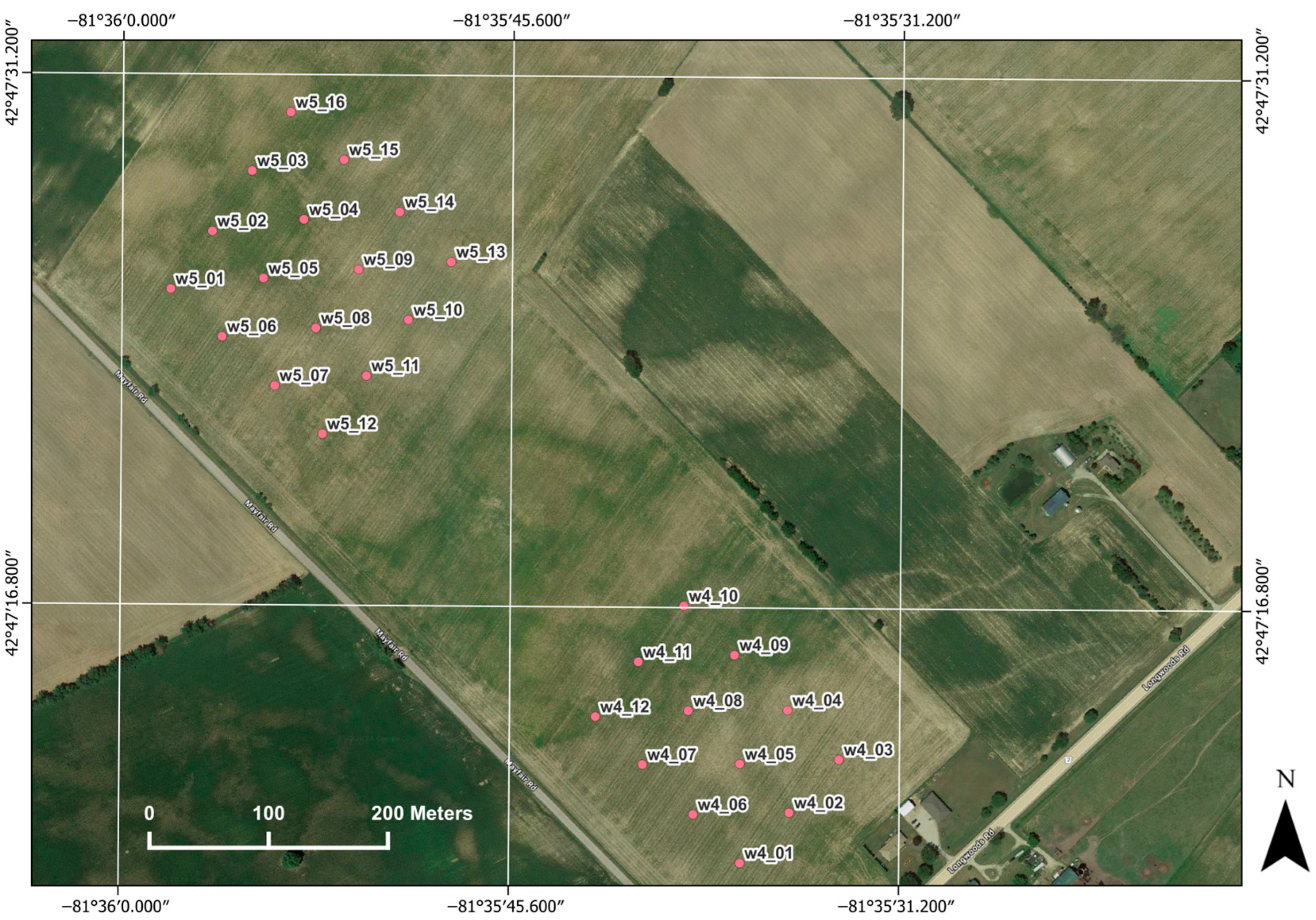
As outlined in Table 1, the field was revisited every six to seven days for ground sampling to align with the changing phenological stages of the winter wheat. Ground sampling was scheduled to align with UAV flights, whenever possible, to maintain consistency in data collection relative to the growth stages. However, optimal conditions for ground sampling and UAV flights were not always synchronized due to potential adverse weather conditions, such as strong winds or rapid weather changes. Given the field’s longest edge exceeding 850 m, two separate UAV flights were necessitated during each visit. Within the map depicted in Figure 2, 2 sets of sampling points were established: 16 sample points in a 4 × 4 grid on the northwest side and 12 sample points in a 4 × 3 grid on the southeast side. This placement aimed to maximize area coverage while minimizing labor intensity. The sampling points were positioned approximately 60 m apart, both vertically and horizontally, to ensure a representative distribution of data. A minimum distance of 50 m from all roads and houses was maintained to mitigate potential outliers and minimize disturbance to local residents. A GPS device was employed to facilitate precise revisits of these sample points during subsequent fieldwork sessions.
Fresh AGB samples were destructively harvested in a 20 × 20 cm grid at each sample point and transported to A&L Canada Laboratories for immediate fresh weight determination on the day of collection. Subsequently, these samples were dried in an oven at 60 °C for 48–72 hours. After drying, the biomass was weighed, and the top leaves of the plants were analyzed to determine nutrient content levels using the A&L PT2 plant test. This test provided nutrient content levels expressed in percentages and parts per million (ppm), as well as both actual and expected nutrient content ratios for each sample. The expected ratio serves as a target value for farmers, aimed at enhancing plant quality; it remains consistent across the field but varies according to the growth stage. In contrast, the actual ratio, derived from the actual nutrient content percentages, varied from sample to sample. In this study, both nutrient content levels and the actual ratio were utilized as biochemical parameters for predicting AGB. For the purposes of this paper, the actual ratio will simply be referred to as “ratio,” as the expected ratio is not utilized in this study.
Additionally, the LAI and crop heights were measured at each sample point as physiological parameters for the machine learning models. A LI-COR LAI-2200C equipped with a 180° view cap was utilized to measure a single LAI value at each sample point as the canopy of the wheat field densified approaching crop maturity. At each sample point, a recording sequence was employed, consisting of four readings above the canopy and eight readings below the canopy near the plant roots, distributed evenly with four in one row and four in the adjacent row. Scattering corrections were applied as needed during the above canopy recording procedures, contingent on ambient lighting and sky conditions. Furthermore, six individual plant height values were measured within a 1 m radius of each sample point using a meter stick, from which an average height value was calculated for each point. During the height measurements, the plants were left undisturbed to maintain their natural posture.

2.2. UAV Imagery

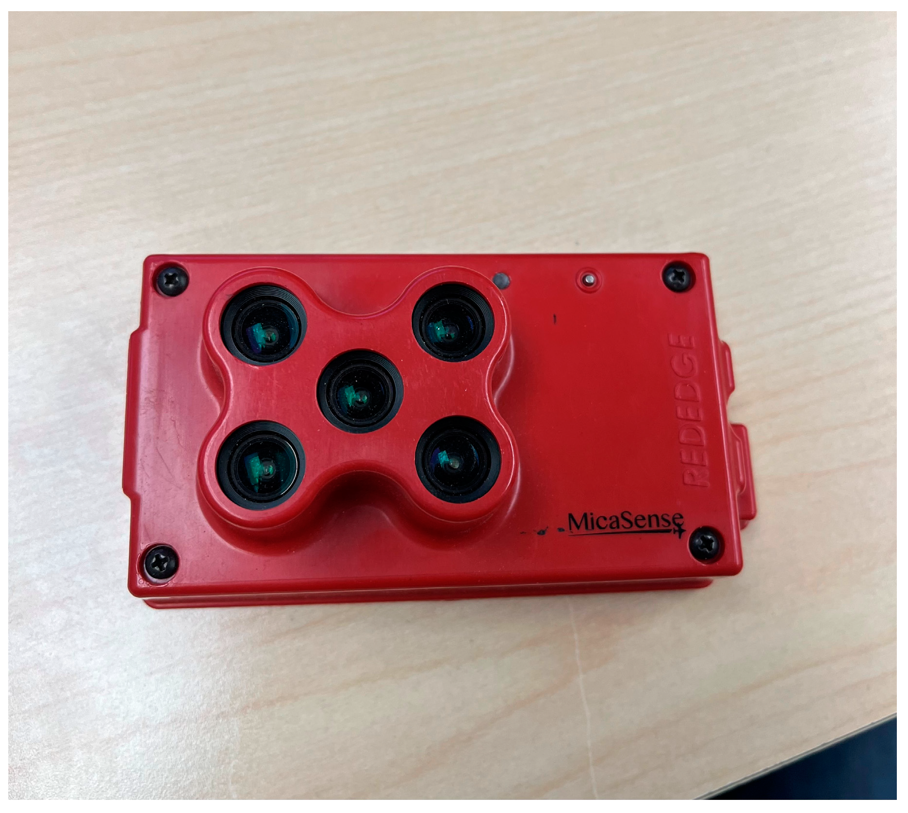
The UAV employed in this study was the Da-Jiang Innovations (DJI) Matrice 100, equipped with a MicaSense RedEdge narrowband multispectral camera (MicaSense Inc., Seattle, WA, USA), which collected spectral information across various bands (Figure 3). All flights were scheduled between 10 a.m. and 2 p.m. under cloud-free or near cloud-free conditions to minimize illumination variability across the field. Flights were postponed and rescheduled to the nearest possible date if the weather conditions were suboptimal, ensuring alignment with ground data collection and the phenological stages of plant growth. Additionally, flights were conducted under the lowest possible wind conditions to reduce challenges in image mosaicking due to plant movement. The flight plan was designed using the Pix4Dcapture app, which allows the pilot to adjust flight settings dynamically. At both sections (W4 and W5) of the study field, flights were conducted at altitudes of 50–60 m above ground level, often at the upper limits of the UAV’s manufacturer-recommended wind speeds. To preserve the data quality and flight efficiency, the UAV was set to fly at speeds between 3 to 4 m/s, depending on the windspeeds of the day. As the winter wheat matured and increased in height, the plants exhibited greater sway. Consequently, to ensure the accuracy of the resulting orthomosaics, all flights were performed with 85% front and side overlapping image capture. The flight paths were executed in a zigzag pattern, aligning with the orientation of the crop rows to enhance the accuracy of the orthomosaics. The outputs were weekly generated MicaSense band orthomosaics with a spatial resolution of 4 × 4 cm. Unfortunately, the flight data collected in the first week experienced a four-day delay relative to the sampling date due to adverse flight conditions. On June 4th, thin clouds scattered across the sky led to the initial assessment of the flight data as inaccurate, followed by three days of intermittent showers or wind speeds too high for safe UAV operation.

2.3. UAV Image Processing

Pix4Dmapper (version 4.8.0) was employed to process the multispectral images collected, generating one orthomosaic image per band. Prior to each flight, the MicaSense camera was subjected to a radiometric calibration to ensure the accuracy of the reflectance data. This calibration involved positioning the camera above a MicaSense Calibrated Reflectance Panel to capture white reference images for each band, taking into account sensor influences and the scene’s illumination conditions at the location. These white reference images, along with the reflectance values provided by the manufacturer’s white board, were utilized in Pix4Dmapper for image calibration, enabling each of the five MicaSense bands to produce corrected reflectance data of the field. The process of Structure from Motion (SfM), utilized by Pix4Dmapper, stitches together all the individual images captured by the camera. The high-overlapping image capture settings established for the flights facilitated this process, enhancing the accuracy of the results. The output comprised five orthomosaic images, each representing different reflectance values across the bands for both sections of the study area.

2.4. Vegetation Indices

The orthomosaic images were used to calculate vegetation indices (VIs) in QGIS. In order to minimize GPS error in the weekly visit to the field sample points, the VI values were averaged within a 1 m radius of the sample point. Details of the camera bands are listed in Table 2.
A total of 13 Vis were calculated, as listed in Table 3. Indices such as the NDVI and SAVI have been previously validated as reliable predictors of winter wheat biomass [22]. Additionally, several of the VIs make use of spectral information in the red edge and near-infrared wavelengths, which have been demonstrated to correlate strongly with crop growth, health, yield, and the LAI [11,32]. The chlorophyll index red edge (CL_RE) has been established as an effective VI for predicting crop nitrogen content, which serves as an indicator of plant vigor and productivity.

2.5. Biochemical Parameters

In this study, 14 nutrient content levels and 8 derived nutrient content ratios were analyzed. Existing research has identified nitrogen and phosphorus as essential for protein synthesis, enzyme activities, and chlorophyll formation in plants [46,47]. Additionally, potassium is crucial in mitigating stress from drought, cold temperatures, salinity, and biotic factors, such as diseases and pests [48]. For example, sufficient potassium levels can enhance photosynthetic efficiency, improve water usage, and stabilize plant metabolism under drought conditions. Additionally, nutrient content ratios, such as nitrogen to sulfur (N:S) in plant leaves, are significant indicators of crop health and nutrient deficiency [49,50]. This framework provided the basis for testing both individual nutrient content levels and ratios. The 14 nutrients tested included nitrogen (N), phosphorus (P), potassium (K), magnesium (Mg), calcium (Ca), sodium (Na), sulfur (S), boron (B), zinc (Zn), manganese (Mn), iron (Fe), copper (Cu), aluminum (Al), and nitrate-N. The 8 nutrient content ratios evaluated were N:S, N:K, P:S, P:Zn, K:Mg, K:Mn, Ca:B, and Fe:Mn.

2.6. Machine Learning Regression Modeling

In the context of machine learning, regression models are used to predict continuous outcomes based on input variables. Two prominent techniques within this domain are Random Forest (RF) Regression and Support Vector Regression (SVR), both of which offer robust solutions to complex regression problems.
RF is an ensemble learning method that operates by constructing multiple decision trees during the calibration phase and outputting the mean prediction of the individual trees. This method capitalizes on the power of multiple decision trees to reduce overfitting, which is common in models relying on a single decision tree. Each tree in the forest is built from a random sample of the calibration data, and at each node, a subset of features is randomly chosen to decide the split. This randomness helps in making the model more resilient to noise in the dataset. Moreover, Random Forest can handle large datasets with higher dimensionality and can estimate which variables are important in the underlying relationships being modeled.
SVR, on the other hand, extends the concepts of Support Vector Machines (SVMs) from classification to regression. Unlike traditional methods that minimize the error between predicted and actual values, SVR attempts to fit the error within a certain threshold. It involves the creation of a hyperplane in a multidimensional space where the distance between the data points and the hyperplane is minimized, ensuring that errors do not exceed a defined threshold. This makes SVR particularly useful in cases where a margin of tolerance is specified in the predictions. SVR is highly effective in handling non-linear relationships through the use of kernel functions, which map input data into higher-dimensional spaces [51].
Both RF and SVR provide distinct advantages depending on the nature of the data and the specific requirements of the regression task [29]. RF is generally preferred for problems with high-dimensional spaces and large datasets, offering interpretations in terms of feature importance. SVR is advantageous when dealing with datasets where the prediction needs to stay within a certain range and is effective in capturing complex relationships through its kernel trick. When employed thoughtfully, both methods can yield highly accurate predictive models in a wide range of scientific and industrial applications.
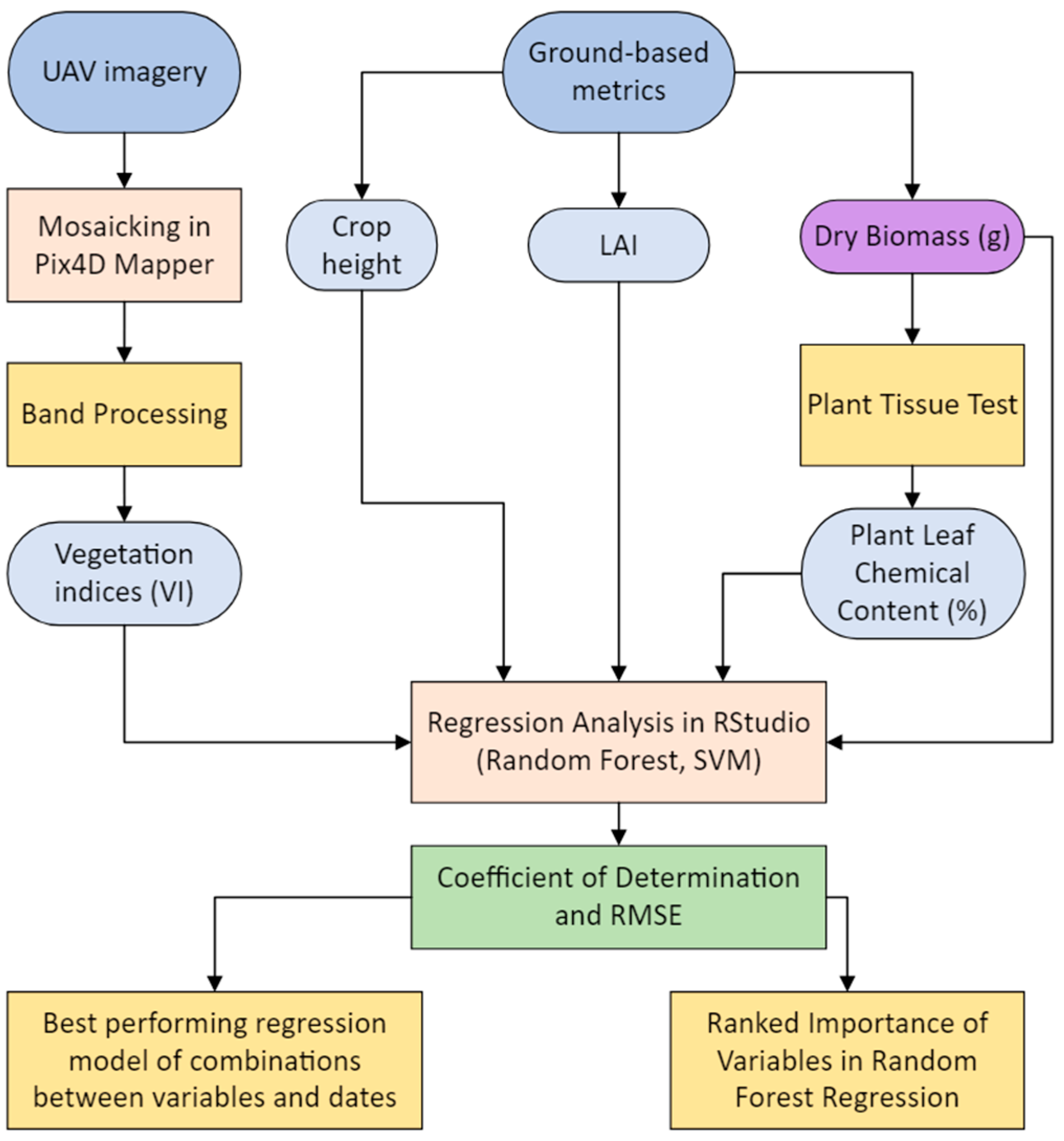
Figure 4 displays the workflow of the methodology. The modeling was written in R programming language using R Studio by utilizing packages such as “randomForest” and “e1071” for RF and SVR, respectively. In both models, the independent variables were the VIs, MicaSense bands, plant physiological parameters, plant nutrient levels, and plant nutrient content ratios. Data collected over the four weeks were randomly divided into a 70% calibration set and a 30% validation set. The strength of the prediction model was assessed using the coefficient of determination (R2) and root mean square error (RMSE). To ensure the model’s strength and generalizability, we validated the results by creating random splits of the calibration and validation sets 100 times. The R2 and RMSE values reported are the average values obtained from these splits. The equations for both metrics are as follows:
R 2 = 1 y i y ^ i 2 y i y - i 2
where y i is the observed value, y ^ i is the predicted value, and y - i is the mean of the observed values, and
RMSE = i = 1 n ( y ^ i y i ) 2 n
where y ^ i represents the predicted AGB (g/m2), y i denotes the observed AGB (g/m2), n is the total number of observations, and i serves as the summation index, incrementing by one.

3. Results

3.1. Biomass Data

AGB was destructively collected at each sample point. The dry weight of the sampled biomass progressively increased across different growth stages, as illustrated in Figure 5. Initially, AGB exhibited a modest increase during the first two weeks of fieldwork, followed by a significant acceleration in growth thereafter.

3.2. Regression Models with All Variables

A total of 42 variables were utilized as predictors for AGB, including plant height, LAI, MicaSense bands, VIs, and levels and ratios of plant nutrient content. The datasets were categorized into single-date and multi-date groups to assess the temporal impact on the models and to identify the most effective date or combination of dates for estimating AGB. These variables were incorporated into the calibration and validation of the RF and SVR models, as detailed in Table 4. Overall, the RF models exhibited slightly superior performance compared to the SVR models, with multi-date RF models outperforming those based on single dates. The best-performing RF model, which utilized all variables across all four dates, achieved an R2 of 0.93 and an RMSE of 90.98 g/m2 in its calibration set, and an R2 of 0.80 with an RMSE of 152.71 g/m2 in its validation set. RF models that incorporated data from three dates also demonstrated high performance. Similarly, SVR models showed improved performance with multi-date data compared to single-date models. The optimal SVR model, employing all variables and data from June 10, 17, and 23, yielded an R2 of 0.90 and an RMSE of 108.79 g/m2 in its calibration set, and an R2 of 0.77 with an RMSE of 156.61 g/m2 in its validation set. Although this model was only marginally superior to its counterpart, which utilized data from all four dates, it featured a lower RMSE. It is noteworthy that almost all models based on single-date data were not significant, a result anticipated due to the high number of variables relative to the modest dataset size of 28 entries.
It is crucial to note that the overall best-performing model is not necessarily the one with the highest R2 value in either the calibration or validation sets. For example, the RF model using data from June 10 and 23 demonstrated a high R2 of 0.97 and a low RMSE of 75.91 g/m2 in the calibration set. However, the same model exhibited significantly weaker performance in the validation set, with an R2 of 0.66 and a high RMSE of 212.96 g/m2. This discrepancy suggests potential overfitting, indicating that while the model predicts the calibration data exceptionally well, it does not generalize effectively to new, unseen data.

3.3. Variable Importance Plot

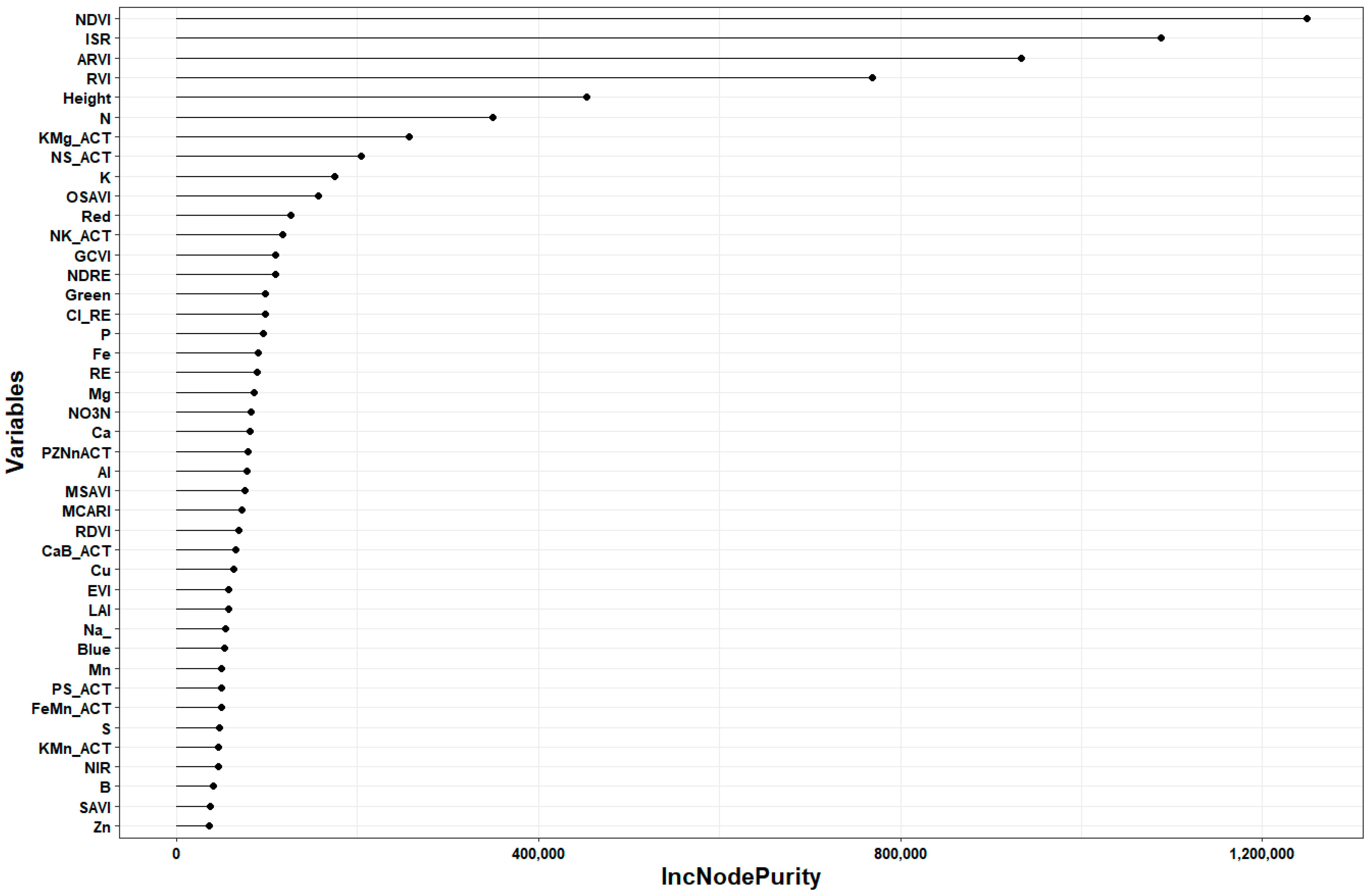
RF modeling, which involves the use of numerous decision trees, was employed to generate a variable importance plot in R Studio using the “varImpPlot()” function. The plot displays increasing node purity (IncNodePurity) on the x-axis, which indicates the importance of each explanatory variable in predicting dry AGB on the decision trees. A higher IncNodePurity value signifies that the variable is more critical as a predictor. This method was employed to visualize the variable rankings in both the RF and SVR models, aiding in the identification of key predictors in the models.
The RF model incorporating all 42 variables demonstrated optimal performance when applied to the full four-date dataset. Analysis of the variable importance plot revealed that the NDVI was the most critical predictor, as depicted in Figure 6. Among the top ten most influential variables, the composition included five of the thirteen VIs utilized, two out of fourteen nutrient content levels, two of the eight nutrient content ratios, and plant height. Notably, the NDVI, ISR, ARVI, and RVI exhibited significantly higher IncNodePurity values compared to the remaining variables. These VIs are commonly associated with vegetation monitoring in agriculture and biomass estimation. Macronutrients such as N and K were also ranked in the top 10. N and K are crucial macronutrients that regulate enzymes and the synthesis of organic compounds. Additionally, K plays a vital role in cell growth and the regulation of photosynthesis, both of which are responsible for plant development [13,48].
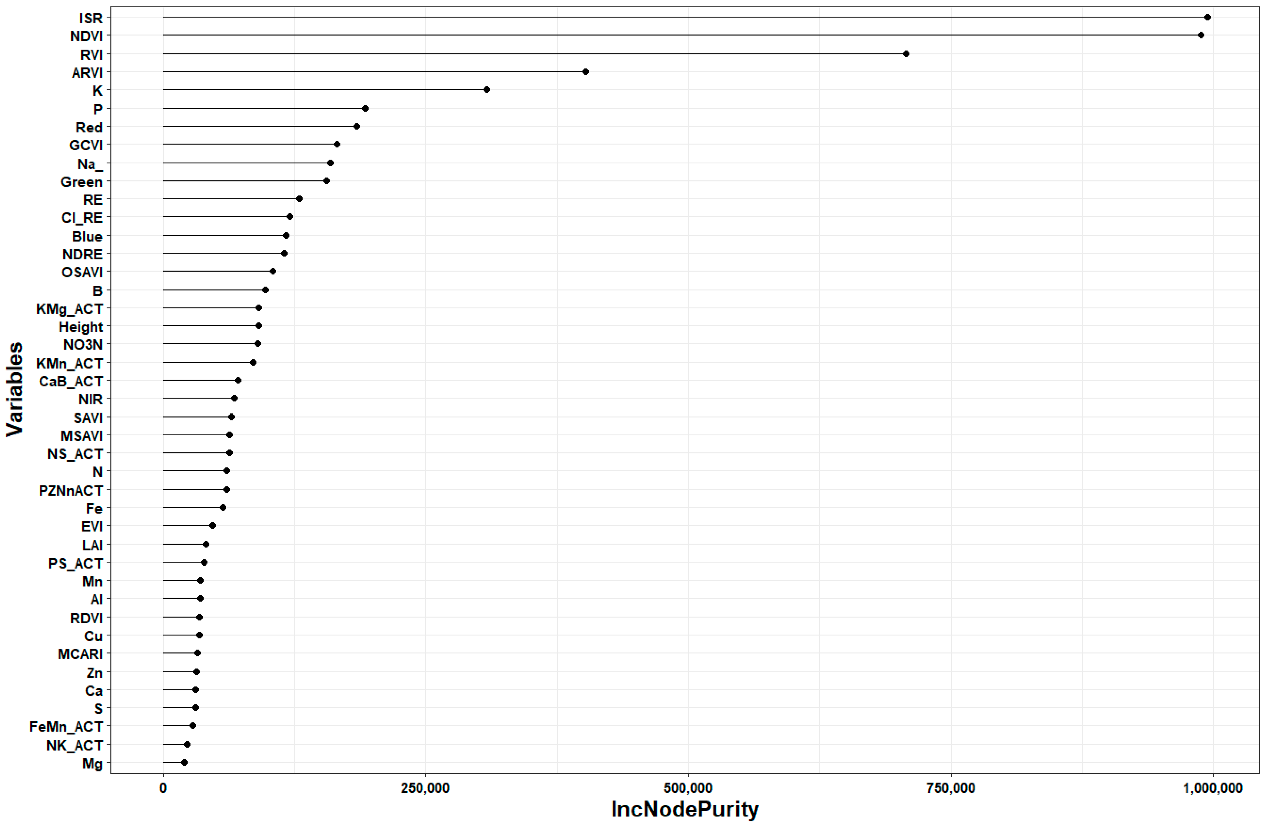
The SVR model that incorporated all 42 variables yielded the best results using data collected on June 10, 17, and 23. A variable importance plot generated from these three dates identified the ISR as the most crucial predictor of AGB, with a slightly higher ranking than the NDVI, as shown in Figure 7. The top ten most important variables included five of the thirteen VIs utilized, three of the fourteen nutrient content levels, and two of the five MicaSense bands. Indices such as the NDVI, ISR, ARVI, and RVI displayed significantly higher IncNodePurity values than the other variables. Consistent with the results from the four-date analysis, the primary predictors remained the ISR, NDVI, RVI, and ARVI, albeit in a different order. In this three-date plot, MicaSense red and green bands, along with P, saw an increase in their rankings, moving into the top ten, a shift from their positions in the four-date plot. P is an essential macronutrient similar to N and K. However, its relevance had only increased in the four-date plot, while the importance of N and K had decreased. P is responsible for various biochemical reactions within the plant, including nitrogen fixation and the synthesis of nucleic acids and phospholipids, making it essential for the genetic and structural components of plant cells [13]. Although KMg_ACT was the highest-ranked nutrient content ratio in both plots, none of the nutrient content ratios were among the top ten variables in the three-date analysis.

3.4. Regression Models with Selected Variables

Variable selection is essential for reducing redundancy and complexity in regression models with a larger variety of variables. It enhances model performance and interpretability by focusing on the most relevant predictors, thereby reducing overfitting and computational complexity. This process also improves the model’s ability to generalize well to new data, ensuring more robust and accurate predictions. As indicated by the variable importance plots (Figure 6 and Figure 7), although the best-performing RF and SVR models utilized all 42 variables, the importance of the explanatory variables in estimating AGB varied considerably. For the RF models, based on the variable importance plot in Figure 6, we selected the top four, seven, ten, fourteen, twenty, and twenty-nine variables, determined by significant reductions in the increase in node purity, which helped establish a ranking threshold. A similar selection process was applied to the SVR models, grouping variables into rankings of the top five, seven, ten, fourteen, twenty, and twenty-eight based on the variable importance plot in Figure 7.
Additionally, two distinct groups of variables were evaluated in both RF and SVR models. Research has substantiated that UAV multispectral data alone can effectively predict AGB, leading to the testing of a class consisting solely of MicaSense bands and VIs [52]. Moreover, plant nutrient content, though seldom used as a predictor for AGB, displayed high importance in some explanatory variables. Consequently, nutrient content levels and ratios were also explored as a separate class for testing.
Table 5 outlines the statistics for RF model calibration and validation sets using data from various dates and combinations of variables. The most effective date combination for RF utilized data from all four dates. For the calibration sets, the R2 remained high across most groups, consistently above 0.9, except for the group containing only the top four variables. The RMSE values ranged from 89.19 to 119.81 g/m2. Notably, the RMSE values were significantly elevated for groups comprising solely multispectral data and VIs, as well as those limited to plant nutrient content levels and ratios, with both exceeding 100 g/m2. A decreasing trend in the RMSE was observed as more variables were included in the calibration sets, continuing up to the top 20 variables. Although the calibration sets exhibited similar performance, the validation set using only multispectral data and VIs outperformed the set that included only plant nutrient content levels and ratios. Nevertheless, neither was the best performing among the RF models. The validation set with the top seven variables demonstrated higher performance, which continued to improve up to the model incorporating the top twenty variables. The validation sets exhibited R2 values between 0.59 and 0.81, with RMSE values spanning from 149.95 to 213.49 g/m2.
The overall best-performing RF model employed a combination of the top 20 variables, achieving an R2 of 0.93 and an RMSE of 89.19 g/m2 in the calibration set and an R2 of 0.81 and an RMSE of 149.95 g/m2 in the validation set. Analyses of the models with the top 29 variables and all 42 variables (as detailed in Table 4) indicated a decline in model performance with the addition of more variables. The R2 values plateaued while the RMSE increased, suggesting that eliminating lower-ranked variables from the variable importance plot can enhance the performance of the RF models.
Table 6 presents the statistics for SVR models using data from June 10, 17, and 23 across various variable combinations. The calibration sets of the SVR models displayed a range of performance with R2 values between 0.72 and 0.88 and RMSE values from 119.65 to 178.05 g/m2. The highest performance was observed with the top twenty-eight variables and the lowest with the top five variables. There was a linear increase in R2 and a corresponding decrease in the RMSE as the number of variables in the calibration sets increased. Unlike the calibration sets, the validation sets did not exhibit consistent trends, with R2 values ranging from 0.62 to 0.77 and RMSE values between 154.36 and 206.40 g/m2. In contrast to the RF models, the SVR model utilizing only multispectral data and VIs performed worse than the model focusing solely on plant nutrient content levels and ratios. However, neither of these models achieved the highest performance.
The best overall performing SVR model utilized the top 28 variables, achieving an R2 of 0.88 and an RMSE of 119.65 g/m2 in the calibration set and an R2 of 0.77 and an RMSE of 154.36 g/m2 in the validation set. Comparing the performance of the model with the top 28 variables to that using all 42 variables (as detailed in Table 4), the former exhibited slightly better generalization capabilities, as indicated by a lower RMSE in the validation set. Therefore, the SVR model with 28 variables was considered superior due to its slightly better balance between training accuracy and validation error. Nonetheless, the differences in validation performance were minimal, suggesting that both models are relatively comparable in their ability to generalize.

4. Discussion

In this study, RF and SVM regression methods were used to predict the AGB of winter wheat, utilizing UAV multispectral MicaSense bands, associated VIs, plant biophysical parameters (plant height and the LAI), and plant biochemical parameters (nutrient content levels and ratios). During the first two weeks of sampling, the variation in AGB was low; however, it began to increase rapidly starting from the third sampling date, June 17. This rapid change aligns with the growth stages of winter wheat. On June 4 and 10, the plants were in their late heading and early flowering stages, respectively—a transition period marked by a slowdown in height increase due to shifts in developmental priorities and physiological changes. Initially, plant height and leaf area are major contributors to AGB as the stem elongates and leaves enlarge. By the heading stage, most stem elongation is complete, with culms extended and plant height largely established. What follows is primarily the emergence of the inflorescence from the flag leaf’s sheath, which does not significantly contribute to further height increase. As the plant transitions to the reproductive phase, its focus shifts from vegetative to reproductive growth, including the formation and maturation of the inflorescence. On June 17, the winter wheat entered the fruit development stage, channeling photosynthates from leaves and stems into the developing grains, which accumulate starch, proteins, and other nutrients, significantly increasing their weight and overall biomass. Finally, during the ripening stage on June 23, the grains transform from a watery, milky substance into a hard, dry state—a process marked by the continuous accumulation of dry matter, primarily starch, enhancing total AGB.
The RF and SVR models were initially calibrated using all 42 variables across single- and multi-date datasets. In the validation sets, models based on single dates generally performed poorly and were statistically non-significant. Our finding agrees with Atkinson Amorim et al.’s work that models using multiple date combinations performed better, especially if the combinations involved the last two dates [27]. The best performance was observed in the RF model that utilized data from all four dates. According to the corresponding variable importance plot, the NDVI emerged as the most crucial variable, with other top-ranked variables primarily consisting of multispectral data. This finding aligns with Fu et al.’s findings that the NDVI and its narrowband-modified variations were effective predictors of biomass using partial least squares regression. Moreover, the top-ranked VIs in AGB estimation mainly comprised the NIR band, further supporting Fu et al.‘s identification of NIR as a sensitive band region for AGB [22]. In PA, employing UAVs equipped with spectral cameras is a common and cost-effective method to capture multispectral data and estimate AGB [53,54,55]. Although previous studies have proposed new methods for estimating crop AGB using multispectral data, our study demonstrates that existing machine learning methods can also produce comparable results when increasing the variety of predictors, such as plant nutrient content levels and ratios. Furthermore, senescence might affect the use of multispectral data for crop biomass monitoring at post-flowering stages, potentially reducing model performance compared to pre-flowering stages [56]. Our study did not encounter this issue, likely due to the inclusion of additional variables beyond multispectral data and derived VIs.
We successfully optimized the machine learning models by selecting the top-ranked variables from the variable importance plots. This approach is consistent with findings from other research, which has proven that machine learning is an effective method for predicting biomass in crops, such as wheat and oats [27,28,56]. While we were using a very similar camera setup installed on the UAV as Sharma et al., our findings proved that including biophysical and biochemical parameters in the analysis can significantly increase the RF and SVR models’ accuracy [56]. Similar to the results of Lu et al., the best-performing RF model proved more accurate than the top SVR model [57]. We tested a total of 42 variables. Although the SVR model performed well, nearly matching the RF model, the latter was better in terms of performance and ease of use. In the RF model, the top twenty variables were selected, which included eight of the thirteen VIs, three of the five MicaSense bands, five of the fourteen nutrient content levels, three of the eight nutrient content ratios, and plant height as the model’s performance started dropping with more variables being added. In comparison, Wang et al. reported higher RMSE values in their post-flowering stage analysis than ours in their linear regression, partial least squares regression (PLSR), and RF models [28]. Our model performance was comparable with theirs, and the lower RMSE values in our models could be advantageous for making timely adjustments in fertilizer and water application recommendations. This is especially crucial in unstable climate conditions, where late-stage growth adjustments are necessary. The RF method, which utilizes multiple decision trees, seems particularly well-suited to handling a high number of variables and avoiding overfitting. As reported by Wang et al., RF outperformed linear regression and PLSR by having higher stability in predicting AGB during their study period. Our findings aligned with theirs, as RF proved to be the more stable model when handling a variety of data compared to SVR. Conversely, the SVR model required user hyper-tuning and used a kernel trick function to separate data into groups, relying on the radial distance between points to provide meaningful insights for the model. We believe that our research findings can be applied to North American wheat fields located at similar latitudes to southern Ontario, Canada. However, the model may perform differently under varying agricultural practices and environmental conditions. Future applications of these findings should take these factors into account.

5. Conclusions

5.1. Contributions of Utilizing Multiple Categories of Variables in AGB Estimation

This study tested the effectiveness of multispectral data and biophysical and biochemical parameters in predicting the AGB of winter wheat using machine learning methods. Variables tested include UAV MicaSense bands, the derived VIs, plant height, the LAI, and plant nutrient content levels and ratios. The best result was obtained from the RF model with an R2 of 0.81 and an RMSE of 149.95 g/m2 using the top 20 variables, with a close to even split between spectral variables and nutrient content variables.
The inclusion of plant nutrient content levels and ratios as predictors in this study represents an advancement in the field of biomass estimation. Traditionally, these variables are not commonly utilized. The utilization of a lower-cost UAV multispectral camera setup, combined with biophysical and biochemical parameters, particularly at the later growth stages of winter wheat post-flowering, demonstrates a cost-effective method to predict AGB when urgent changes in late growth stages are needed to counteract unpredicted weather events, such as forest fire smoke and haze.

5.2. Limitations and Future Work

Though machine learning algorithms are capable of analyzing variables across categories, it is important to recognize the empirical nature of the machine learning models used. These models, by design, rely on existing datasets for validation and can only approximate the true AGB, which is only verifiable at harvest. This intrinsic limitation highlights the potential discrepancies between predicted and actual outcomes. Such limitations underscore the necessity for ongoing calibration and testing of these models under varied agricultural conditions and across different crop cycles to ensure their reliability and accuracy. The applications of these models can also be limited to dataset access, which is a common limitation in PA research because in situ measurements often are required, and that comes with the associated intensive labor, costs, and conditions. Additionally, it is important to recognize that the variables tested are not the only associated factors that affect AGB. Variables such as weather conditions, soil properties, field topography, moisture supply, and more need to be considered to define the condition of the plants.
Due to constraints in data and time availability, this research could not be conducted earlier in the growth stages of the winter wheat. Future studies should consider extending the time span to investigate the models’ effectiveness more comprehensively. Additionally, further exploration into the use of UAV-based spectral data for biomass estimation is suggested. This exploration should particularly focus on wavelengths or VIs that strongly correlate with plant nutrient levels and ratios. More importantly, it should emphasize hyperspectral bands, which have proven to be highly accurate in monitoring crop growth and estimating yield [58]. Furthermore, high spatial and temporal resolution satellite imagery can serve as a viable alternative to UAV imagery, eliminating the need for UAVs. Examples such as Planetscope and VENμS both have frequent revisit periods and high spatial resolution for a local, field-scale study. We demonstrated the effectiveness of using plant nutrient content levels and ratios as parameters to estimate AGB in this study. Therefore, further research into non-destructive methods using remote sensing techniques to obtain these data is recommended for future biomass estimation studies. Since plant height has also been proven to be a reliable predictor in this study, integrating Real-Time Kinematic (RTK) UAVs or LiDAR-equipped UAVs could enhance the precision and quantity of height data collection across the entire field. Combining these technologies with biomass estimation models could lead to the development of highly accurate AGB estimation maps, providing a more detailed understanding of biomass and crop yield potential.

Author Contributions

Conceptualization, M.S.C. and J.W.; methodology, M.S.C. and J.W.; software, M.S.C.; validation, J.W.; formal analysis, M.S.C.; investigation, M.S.C.; resources, J.W.; data curation, M.S.C.; writing—original draft preparation, M.S.C.; writing—review and editing, M.S.C. and J.W.; visualization, M.S.C.; supervision, J.W.; project administration, J.W.; funding acquisition, J.W. All authors have read and agreed to the published version of the manuscript.

Funding

This study was funded by the Natural Science and Engineering Research Council of Canada (NSERC) Discovery Grant (grant number RGPIN-2022-05051), awarded to Wang. Additional funding was the Western Graduate Research Scholarship provided by The University of Western Ontario granted to Chiu.

Data Availability Statement

The data collected for this paper are not publicly available.

Acknowledgments

The authors would like to thank A&L Canada Laboratories Inc. and the members of Wang’s GITA lab for their invaluable assistance with data collection, lab processing, and overall support. Special thanks go to Bo Shan, Robin Kwik, Naythan Samuda, Xin Zhou, Chenyang Zhou, Jordan Wogan, Chunhua Liao, and Dora Dmytriyenko for their dedicated help with fieldwork and guidance. Additionally, the authors extend their gratitude to Jody Yu for her expertise and guidance in programming the machine learning analyses. The authors would also like to thank the anonymous reviewers for their time, helpful comments, and feedback on this manuscript.

Conflicts of Interest

The authors declare no conflicts of interest.

References

  1. Tan, C.S.; Reynolds, W.D. Impacts of Recent Climate Trends on Agriculture in Southwestern Ontario. Can. Water Resour. J. 2003, 28, 87–97. [Google Scholar] [CrossRef]
  2. Reid, S.; Smit, B.; Caldwell, W.; Belliveau, S. Vulnerability and Adaptation to Climate Risks in Ontario Agriculture. Mitig. Adapt. Strateg. Glob. Chang. 2007, 12, 609–637. [Google Scholar] [CrossRef]
  3. Government of Canada. Overview of Canada’s Agriculture and Agri-Food Sector; Agriculture and Agri-Food Canada, Canada; 2023; Available online: https://agriculture.canada.ca/en/sector/overview (accessed on 25 May 2024).
  4. Chlingaryan, A.; Sukkarieh, S.; Whelan, B. Machine Learning Approaches for Crop Yield Prediction and Nitrogen Status Estimation in Precision Agriculture: A Review. Comput. Electron. Agric. 2018, 151, 61–69. [Google Scholar] [CrossRef]
  5. Bendig, J.; Yu, K.; Aasen, H.; Bolten, A.; Bennertz, S.; Broscheit, J.; Gnyp, M.L.; Bareth, G. Combining UAV-Based Plant Height from Crop Surface Models, Visible, and near Infrared Vegetation Indices for Biomass Monitoring in Barley. Int. J. Appl. Earth Obs. Geoinf. 2015, 39, 79–87. [Google Scholar] [CrossRef]
  6. Li, W.; Niu, Z.; Huang, N.; Wang, C.; Gao, S.; Wu, C. Airborne LiDAR Technique for Estimating Biomass Components of Maize: A Case Study in Zhangye City, Northwest China. Ecol. Indic. 2015, 57, 486–496. [Google Scholar] [CrossRef]
  7. Bendig, J.; Bolten, A.; Bennertz, S.; Broscheit, J.; Eichfuss, S.; Bareth, G. Estimating Biomass of Barley Using Crop Surface Models (CSMs) Derived from UAV-Based RGB Imaging. Remote Sens. 2014, 6, 10395–10412. [Google Scholar] [CrossRef]
  8. Guo, Y.; He, J.; Zhang, H.; Shi, Z.; Wei, P.; Jing, Y.; Yang, X.; Zhang, Y.; Wang, L.; Zheng, G. Improvement of Winter Wheat Aboveground Biomass Estimation Using Digital Surface Model Information Extracted from Unmanned-Aerial-Vehicle-Based Multispectral Images. Agriculture 2024, 14, 378. [Google Scholar] [CrossRef]
  9. Liu, J.; Pattey, E.; Miller, J.R.; McNairn, H.; Smith, A.; Hu, B. Estimating Crop Stresses, Aboveground Dry Biomass and Yield of Corn Using Multi-Temporal Optical Data Combined with a Radiation Use Efficiency Model. Remote Sens. Environ. 2010, 114, 1167–1177. [Google Scholar] [CrossRef]
  10. Tian, J.; Wang, S.; Zhang, L.; Wu, T.; She, X.; Jiang, H. Evaluating Different Vegetation Index for Estimating Lai of Winter Wheat Using Hyperspectral Remote Sensing Data. In Proceedings of the 2015 7th Workshop on Hyperspectral Image and Signal Processing: Evolution in Remote Sensing (WHISPERS), Tokyo, Japan, 2–5 June 2015; pp. 1–4. [Google Scholar] [CrossRef]
  11. Xie, Q.; Huang, W.; Liang, D.; Chen, P.; Wu, C.; Yang, G.; Zhang, J.; Huang, L.; Zhang, D. Leaf Area Index Estimation Using Vegetation Indices Derived from Airborne Hyperspectral Images in Winter Wheat. IEEE J. Sel. Top. Appl. Earth Obs. Remote Sens. 2014, 7, 3586–3594. [Google Scholar] [CrossRef]
  12. Cavender-Bares, J.; Gamon, J.A.; Townsend, P.A. (Eds.) Remote Sensing of Plant Biodiversity; Springer Nature: Cham, Switzerland, 2020. [Google Scholar] [CrossRef]
  13. Marschner, H. Marschner’s Mineral Nutrition of Higher Plants, 3rd ed.; Academic Press: Waltham, MA, USA, 2011; ISBN 978-0-12-384905-2. [Google Scholar]
  14. Bryant, C.R.; Smit, B.; Brklacich, M.; Johnston, T.R.; Smithers, J.; Chiotti, Q.; Singh, B. Adaptation in Canadian Agriculture to Climatic Variability and Change. In Societal Adaptation to Climate Variability and Change; Kane, S.M., Yohe, G.W., Eds.; Springer Netherlands: Dordrecht, The Netherlands, 2000; pp. 181–201. [Google Scholar] [CrossRef]
  15. Zhao, S.; Lü, J.; Xu, X.; Lin, X.; Luiz, M.R.; Qiu, S.; Ciampitti, I.; He, P. Peanut Yield, Nutrient Uptake and Nutrient Requirements in Different Regions of China. J. Integr. Agric. 2021, 20, 2502–2511. [Google Scholar] [CrossRef]
  16. Koerselman, W.; Meuleman, A.F.M. The Vegetation N:P Ratio: A New Tool to Detect the Nature of Nutrient Limitation. J. Appl. Ecol. 1996, 33, 1441–1450. [Google Scholar] [CrossRef]
  17. Radoglou-Grammatikis, P.; Sarigiannidis, P.; Lagkas, T.; Moscholios, I. A Compilation of UAV Applications for Precision Agriculture. Comput. Netw. 2020, 172, 107148. [Google Scholar] [CrossRef]
  18. Wu, C.; Niu, Z.; Tang, Q.; Huang, W. Estimating Chlorophyll Content from Hyperspectral Vegetation Indices: Modeling and Validation. Agric. For. Meteorol. 2008, 148, 1230–1241. [Google Scholar] [CrossRef]
  19. Yu, J.; Wang, J.; Leblon, B.; Song, Y. Nitrogen Estimation for Wheat Using UAV-Based and Satellite Multispectral Imagery, Topographic Metrics, Leaf Area Index, Plant Height, Soil Moisture, and Machine Learning Methods. Nitrogen 2022, 3, 1–25. [Google Scholar] [CrossRef]
  20. Sishodia, R.P.; Ray, R.L.; Singh, S.K. Applications of Remote Sensing in Precision Agriculture: A Review. Remote Sens. 2020, 12, 3136. [Google Scholar] [CrossRef]
  21. Silleos, N.G.; Alexandridis, T.K.; Gitas, I.Z.; Perakis, K. Vegetation Indices: Advances Made in Biomass Estimation and Vegetation Monitoring in the Last 30 Years. Geocarto Int. 2006, 21, 21–28. [Google Scholar] [CrossRef]
  22. Fu, Y.; Yang, G.; Wang, J.; Song, X.; Feng, H. Winter Wheat Biomass Estimation Based on Spectral Indices, Band Depth Analysis and Partial Least Squares Regression Using Hyperspectral Measurements. Comput. Electron. Agric. 2014, 100, 51–59. [Google Scholar] [CrossRef]
  23. Gómez, D.; Salvador, P.; Sanz, J.; Casanova, J.L. Potato Yield Prediction Using Machine Learning Techniques and Sentinel 2 Data. Remote Sens. 2019, 11, 1745. [Google Scholar] [CrossRef]
  24. Liao, C.; Wang, J.; Shan, B.; Song, Y.; He, Y.; Dong, T. Near Real-time Yield Forecasting of Winter Wheat Using Sentinel-2 Imagery at the Early Stages. Precis. Agric. 2022, 24, 807–829. [Google Scholar] [CrossRef]
  25. Bukowiecki, J.; Rose, T.; Kage, H. Sentinel-2 Data for Precision Agriculture?—A UAV-Based Assessment. Sensors 2021, 21, 2861. [Google Scholar] [CrossRef]
  26. Ontario Ministry of Agriculture, Food and Rural Affairs. Census Farm Data Collection; Ontario Data Catalogue, Canada; 2022; Available online: https://data.ontario.ca/dataset/census-farm-data-collection (accessed on 26 May 2024).
  27. Atkinson Amorim, J.G.; Schreiber, L.V.; de Souza, M.R.Q.; Negreiros, M.; Susin, A.; Bredemeier, C.; Trentin, C.; Vian, A.L.; de Oliveira Andrades-Filho, C.; Doering, D.; et al. Biomass Estimation of Spring Wheat with Machine Learning Methods Using UAV-Based Multispectral Imaging. Int. J. Remote Sens. 2022, 43, 4758–4773. [Google Scholar] [CrossRef]
  28. Wang, F.; Yang, M.; Ma, L.; Zhang, T.; Qin, W.; Li, W.; Zhang, Y.; Sun, Z.; Wang, Z.; Li, F.; et al. Estimation of Above-Ground Biomass of Winter Wheat Based on Consumer-Grade Multi-Spectral UAV. Remote Sens. 2022, 14, 1251. [Google Scholar] [CrossRef]
  29. van Klompenburg, T.; Kassahun, A.; Catal, C. Crop Yield Prediction Using Machine Learning: A Systematic Literature Review. Comput. Electron. Agric. 2020, 177, 105709. [Google Scholar] [CrossRef]
  30. Tausch, R.J. Comparison of Regression Methods for Biomass Estimation of Sagebrush and Bunchgrass. Great Basin Nat. 1989, 49, 373–380. [Google Scholar]
  31. Di Bella, C.M.; Paruelo, J.M.; Becerra, J.E.; Bacour, C.; Baret, F. Effect of Senescent Leaves on NDVI-Based Estimates of fAPAR: Experimental and Modelling Evidences. Int. J. Remote Sens. 2004, 25, 5415–5427. [Google Scholar] [CrossRef]
  32. Zhang, Y.; Qin, Q.; Ren, H.; Sun, Y.; Li, M.; Zhang, T.; Ren, S. Optimal Hyperspectral Characteristics Determination for Winter Wheat Yield Prediction. Remote Sens. 2018, 10, 2015. [Google Scholar] [CrossRef]
  33. Kaufman, Y.J.; Tanre, D. Atmospherically Resistant Vegetation Index (ARVI) for EOS-MODIS. IEEE Trans. Geosci. Remote Sens. 1992, 30, 261–270. [Google Scholar] [CrossRef]
  34. Gitelson, A.A.; Gritz, Y.; Merzlyak, M.N. Relationships between Leaf Chlorophyll Content and Spectral Reflectance and Algorithms for Non-Destructive Chlorophyll Assessment in Higher Plant Leaves. J. Plant Physiol. 2003, 160, 271–282. [Google Scholar] [CrossRef] [PubMed]
  35. Huete, A.; Didan, K.; Miura, T.; Rodriguez, E.P.; Gao, X.; Ferreira, L.G. Overview of the Radiometric and Biophysical Performance of the MODIS Vegetation Indices. Remote Sens. Environ. 2002, 83, 195–213. [Google Scholar] [CrossRef]
  36. Gitelson, A.A.; Viña, A.; Arkebauer, T.J.; Rundquist, D.C.; Keydan, G.; Leavitt, B. Remote Estimation of Leaf Area Index and Green Leaf Biomass in Maize Canopies. Geophys. Res. Lett. 2003, 30, 1248. [Google Scholar] [CrossRef]
  37. Fernandes, R.; Butson, C.; Leblanc, S.; Latifovic, R. Landsat-5 TM and Landsat-7 ETM+ Based Accuracy Assessment of Leaf Area Index Products for Canada Derived from SPOT-4 VEGETATION Data. Can. J. Remote Sens. 2003, 29, 241–258. [Google Scholar] [CrossRef]
  38. Daughtry, C.S.T.; Walthall, C.L.; Kim, M.S.; de Colstoun, E.B.; McMurtrey, J.E. Estimating Corn Leaf Chlorophyll Concentration from Leaf and Canopy Reflectance. Remote Sens. Environ. 2000, 74, 229–239. [Google Scholar] [CrossRef]
  39. Qi, J.; Chehbouni, A.; Huete, A.R.; Kerr, Y.H.; Sorooshian, S. A Modified Soil Adjusted Vegetation Index. Remote Sens. Environ. 1994, 48, 119–126. [Google Scholar] [CrossRef]
  40. Gitelson, A.; Merzlyak, M.N. Quantitative Estimation of Chlorophyll-a Using Reflectance Spectra: Experiments with Autumn Chestnut and Maple Leaves. J. Photochem. Photobiol. B Biol. 1994, 22, 247–252. [Google Scholar] [CrossRef]
  41. Rouse, J.W.; Haas, R.H.; Schell, J.A.; Deering, D.W. Monitoring Vegetation Systems in the Great Plains with ERTS. NASA Spec. Publ. 1974, 351, 309. [Google Scholar]
  42. Rondeaux, G.; Steven, M.; Baret, F. Optimization of Soil-Adjusted Vegetation Indices. Remote Sens. Environ. 1996, 55, 95–107. [Google Scholar] [CrossRef]
  43. Roujean, J.-L.; Breon, F.-M. Estimating PAR Absorbed by Vegetation from Bidirectional Reflectance Measurements. Remote Sens. Environ. 1995, 51, 375–384. [Google Scholar] [CrossRef]
  44. Jordan, C.F. Derivation of Leaf-Area Index from Quality of Light on the Forest Floor. Ecology 1969, 50, 663–666. [Google Scholar] [CrossRef]
  45. Huete, A.R. A Soil-Adjusted Vegetation Index (SAVI). Remote Sens. Environ. 1988, 25, 295–309. [Google Scholar] [CrossRef]
  46. Novoa, R.; Loomis, R.S. Nitrogen and Plant Production. Plant Soil 1981, 58, 177–204. [Google Scholar] [CrossRef]
  47. Shi, Q.; Pang, J.; Yong, J.W.H.; Bai, C.; Pereira, C.G.; Song, Q.; Wu, D.; Dong, Q.; Cheng, X.; Wang, F.; et al. Phosphorus-Fertilisation Has Differential Effects on Leaf Growth and Photosynthetic Capacity of Arachis hypogaea L. Plant Soil 2020, 447, 99–116. [Google Scholar] [CrossRef]
  48. Oosterhuis, D.M.; Loka, D.A.; Kawakami, E.M.; Pettigrew, W.T. The Physiology of Potassium in Crop Production. In Advances in Agronomy; Sparks, D.L., Ed.; Elsevier: Amsterdam, The Netherlands, 2014; Volume 126, pp. 203–233. [Google Scholar] [CrossRef]
  49. Blake-Kalff, M.M.A.; Hawkesford, M.J.; Zhao, F.J.; McGrath, S.P. Diagnosing Sulfur Deficiency in Field-Grown Oilseed Rape (Brassica napus L.) and Wheat (Triticum aestivum L.). Plant Soil 2000, 225, 95–107. [Google Scholar] [CrossRef]
  50. Pagani, A.; Echeverría, H.E. Performance of Sulfur Diagnostic Methods for Corn. Agron. J. 2011, 103, 413–421. [Google Scholar] [CrossRef]
  51. Chang, C.-C.; Lin, C.-J. LIBSVM: A Library for Support Vector Machines. ACM Trans. Intell. Syst. Technol. 2011, 2, 1–27. [Google Scholar] [CrossRef]
  52. Zhu, Y.; Liu, J.; Tao, X.; Su, X.; Li, W.; Zha, H.; Wu, W.; Li, X. A Three-Dimensional Conceptual Model for Estimating the Above-Ground Biomass of Winter Wheat Using Digital and Multispectral Unmanned Aerial Vehicle Images at Various Growth Stages. Remote Sens. 2023, 15, 3332. [Google Scholar] [CrossRef]
  53. Wei, L.; Yang, H.; Niu, Y.; Zhang, Y.; Xu, L.; Chai, X. Wheat Biomass, Yield, and Straw-Grain Ratio Estimation from Multi-Temporal UAV-Based RGB and Multispectral Images. Biosyst. Eng. 2023, 234, 187–205. [Google Scholar] [CrossRef]
  54. Zhang, J.; Zhao, Y.; Hu, Z.; Xiao, W. Unmanned Aerial System-Based Wheat Biomass Estimation Using Multispectral, Structural and Meteorological Data. Agriculture 2023, 13, 1621. [Google Scholar] [CrossRef]
  55. Hassan, M.A.; Yang, M.; Rasheed, A.; Jin, X.; Xia, X.; Xiao, Y.; He, Z. Time-Series Multispectral Indices from Unmanned Aerial Vehicle Imagery Reveal Senescence Rate in Bread Wheat. Remote Sens. 2018, 10, 809. [Google Scholar] [CrossRef]
  56. Sharma, P.; Leigh, L.; Chang, J.; Maimaitijiang, M.; Caffé, M. Above-Ground Biomass Estimation in Oats Using UAV Remote Sensing and Machine Learning. Sensors 2022, 22, 601. [Google Scholar] [CrossRef]
  57. Lu, N.; Zhou, J.; Han, Z.; Li, D.; Cao, Q.; Yao, X.; Tian, Y.; Zhu, Y.; Cao, W.; Cheng, T. Improved Estimation of Aboveground Biomass in Wheat from RGB Imagery and Point Cloud Data Acquired with a Low-Cost Unmanned Aerial Vehicle System. Plant Methods 2019, 15, 17. [Google Scholar] [CrossRef]
  58. Guo, Y.; Xiao, Y.; Hao, F.; Zhang, X.; Chen, J.; de Beurs, K.; He, Y.; Fu, Y.H. Comparison of Different Machine Learning Algorithms for Predicting Maize Grain Yield Using UAV-Based Hyperspectral Images. Int. J. Appl. Earth Obs. Geoinf. 2023, 124, 103528. [Google Scholar] [CrossRef]
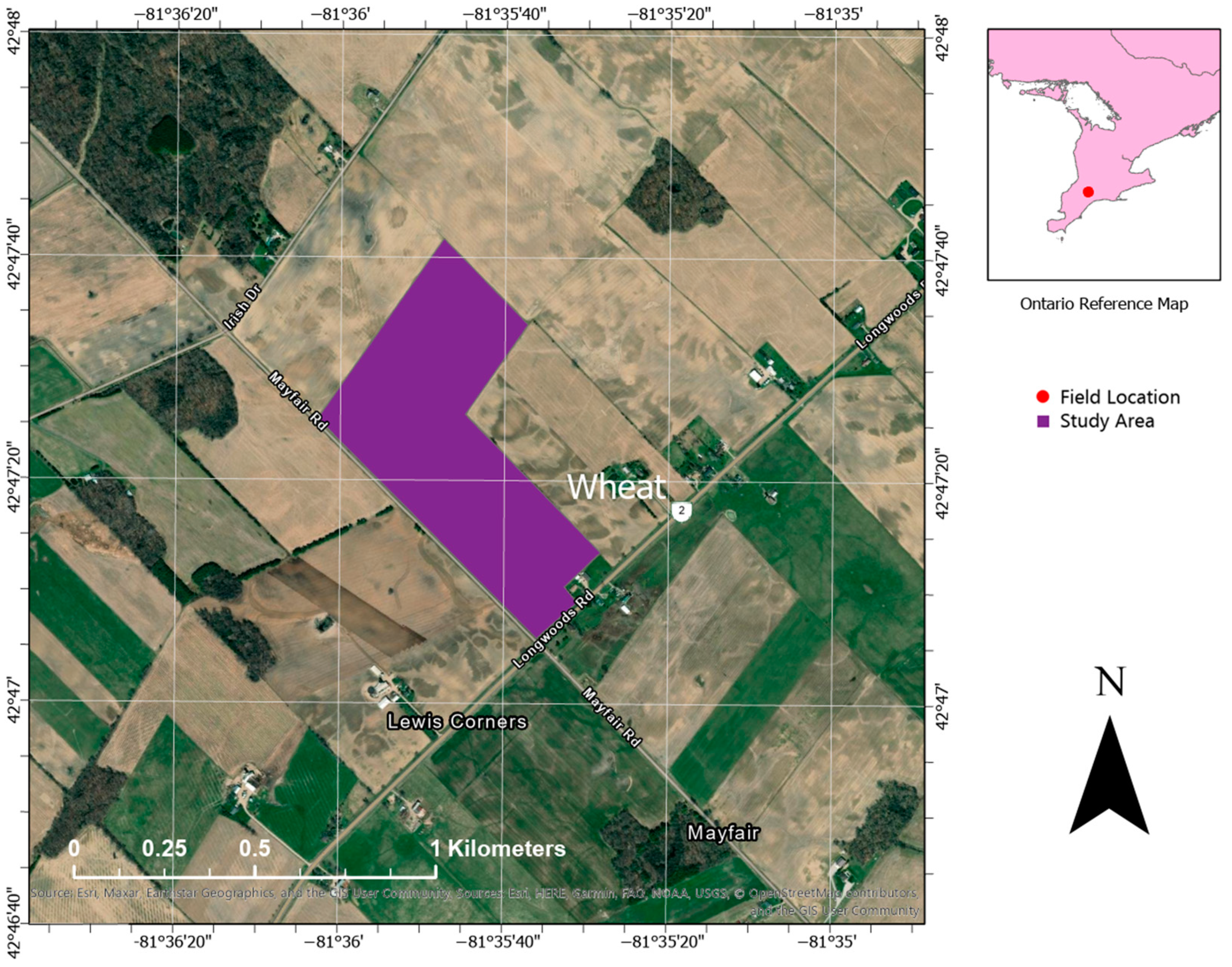
Figure 1. Location of the studied wheat field near Melbourne, ON, Canada over an ArcGIS Pro Basemap Image.
Drones 08 00287 g001
Figure 2. Location and distribution of the sample points.
Drones 08 00287 g002
Figure 3. Image of the MicaSense RedEdge narrowband multispectral camera.
Drones 08 00287 g003
Figure 4. Methodology flowchart of this study.
Drones 08 00287 g004
Figure 5. Distribution of above-ground biomass data throughout the four-week study period during the June 2022 growing season.
Drones 08 00287 g005
Figure 6. Variable importance plot produced with all 42 variables from all four dates. A higher IncNodePurity value indicates a higher impact on AGB estimation. Refer to Table 3 for the full names of vegetation indices. Al, aluminum; B, boron; Ca, calcium; CaB_ACT, calcium boron actual ratio; Cu, copper; Fe, iron; FeMn_ACT, iron manganese actual ratio; K, potassium; KMg_ACT, potassium magnesium actual ratio; KMn_ACT, potassium manganese actual ratio; Mg, magnesium; Mn, manganese; N, nitrogen; Na_, sodium; NK_ACT; nitrogen potassium actual ratio; NO3N, nitrate nitrogen; NS_ACT, nitrogen sulfur actual ratio; P, phosphorus; PS_ACT, phosphorus sulfur actual ratio; PZn_ACT, phosphorus zinc actual ratio; S, sulfur; Zn, zinc.
Drones 08 00287 g006
Figure 7. Variable importance plot produced with all 42 variables from June 10, 17, and 23. A higher IncNodePurity value indicates a higher impact on AGB estimation. Refer to Figure 6 for the full names of the variables.
Drones 08 00287 g007
Table 1. Number of sample points and dates of data collection season.
Fieldwork DatesField Sample Point Groups# of Sample PointsUAV Flight DatesPhenology
(BBCH Scale 1)
June 4Winter Wheat Field W4 and W512 in W4,
16 in W5
June 8Inflorescence emergence, heading (high 50 s to low 60 s)
June 10June 10Flowering, anthesis (60 s)
June 17June 19Development of fruit (70 s)
June 23June 24Ripening (low 80 s)
1 Biologische Bundesanstalt, Bundessortenamt and CHemical industry.
Table 2. Spectral bands of the MicaSense multispectral camera.
BandNameBand Range (nm)Center Wavelength (nm)Bandwidth (nm)
1Blue465–48547520
2Green550–57056020
3Red663–67366810
4Red Edge712–72271710
5NIR820–86084040
Table 3. Vegetation indices to be tested in this study.
VI 1Formula 2Authors
ARVI NIR [ Red 1 × Blue Red ] NIR + [ Red 1 × Blue Red ] Kaufman and Tanre [33]
Cl_RE NIR ÷ RE 1 Gitelson et al. [34]
EVI 2.5 × ( NIR Red ) NIR + 6 × Red - 7.5 × Blue + 1   Huete et al. [35]
GCVI NIR ÷ Green 1 Gitelson et al. [36]
ISR Red ÷ NIR Fernades et al. [37]
MCARI [ RE Red 0.2 × RE Green ] × RE ÷ Red Daughtry et al. [38]
MSAVI [ 2 × NIR + 1 2 × NIR + 1 2 8 × NIR Red ] ÷ 2 Qi et al. [39]
NDRE ( N I R R E ) ÷ ( N I R + R E ) Gitelson and Merzyak [40]
NDVI ( NIR Red ) ÷ ( NIR + Red ) Rouse et al. [41]
OSAVI [ 1.16 × ( NIR Red ) ] ÷ ( NIR + Red + 0.16 ) Rondeaux et al. [42]
RDVI ( NIR Red ) ÷ ( NIR + Red   ) Roujean and Breon [43]
RVI NIR ÷ Red Jordan [44]
SAVI [ 1.5 × ( NIR Red ) ] ÷ ( NIR + Red + 0.5 ) Huete [45]
1 ARVI, atmospherically resistant vegetation index; Cl_RE, chlorophyll index red edge; EVI, enhanced vegetation index; GCVI, green chlorophyll vegetation index; ISR, infrared simple ratio; MCARI, modified chlorophyll absorption in reflectance index; MSAVI, modified soil-adjusted vegetation index; NDRE, normalized difference red edge; NDVI, normalized difference vegetation index; OSAVI, optimized soil-adjusted vegetation index; RDVI, renormalized difference vegetation index; RVI, ratio vegetation index; SAVI, soil-adjusted vegetation index. 2 Blue, blue reflectance; green, green reflectance; red, red reflectance; RE, red edge reflectance; NIR, near-infrared reflectance.
Table 4. Calibration and validation statistics: analysis by date and modeling approach (RF and SVR) using 42 variables, including plant height, the LAI, MicaSense bands, vegetation indices, and plant nutrient content levels and ratios 1. n is the number of data entries.
DateModel(n)CalibrationValidation
R2RMSE (g/m2)R2p-ValueRMSE (g/m2)
June 4RF280.9541.900.21NS137.37
SVR280.9340.110.47<0.05132.17
June 10RF280.9654.64−0.13NS86.19
SVR280.8558.74−0.14NS99.63
June 17RF280.9352.62−0.02NS162.74
SVR280.7676.20−0.14NS132.08
June 23RF280.9580.82−0.14NS245.32
SVR280.70113.80−0.14NS238.80
June 4, 10RF560.9544.03−0.06NS134.58
SVR560.7563.900.09NS130.63
June 4, 17RF560.9460.620.57<0.001138.11
SVR560.8577.200.470.001155.47
June 4, 23RF560.9775.910.68<0.001237.24
SVR560.9683.870.59<0.001257.60
June 10, 17RF560.9259.010.40<0.01123.23
SVR560.8471.790.460.001120.43
June 10, 23RF560.9771.460.66<0.001212.96
SVR560.9683.510.68<0.001201.40
June 17, 23RF560.9486.270.23<0.05252.59
SVR560.90103.300.22<0.05249.10
June 4, 10, 17RF840.9458.610.41<0.001131.64
SVR840.8473.800.38<0.001130.17
June 4, 10, 23RF840.9682.960.67<0.001207.08
SVR840.9498.080.71<0.001184.32
June 4, 17, 23RF840.9491.830.76<0.001177.09
SVR840.90112.880.72<0.001187.79
June 10, 17, 23RF840.9489.500.72<0.001177.91
SVR840.90108.790.77<0.001156.61
June 4, 10, 17, 23RF1120.9390.980.80<0.001152.71
SVR1120.89113.810.77<0.001165.71
1 All calibration models are significant at p-value < 0.001.
Table 5. Statistics of the RF models for above-ground biomass estimation with all dates (June 4, 10, 17, 23) and different combinations of variables (n = 112) 1.
VariablesNumber of VariablesCalibrationValidation
R2RMSE (g/m2)R2RMSE (g/m2)
All VIs + 5 MicaSense bands180.91102.190.73175.63
All plant nutrient content + ratios220.93100.790.68196.54
Top 4: NDVI, ISR, ARVI, RVI40.87119.810.59213.49
Top 7: top 4 + height, N, KMg_ACT70.91100.900.76167.32
Top 10: top 7 + NS_ACT, K, OSAVI100.9392.360.79156.00
Top 14: Top 10 + red, NK_ACT, GCVI, NDRE140.9389.530.78160.04
Top 20: Top 14 + green, Cl_RE, P, Fe, RE, Mg200.9389.190.81149.95
Top 29: top 20 + NO3N, Ca, PZn_ACT, Al, MSAVI, MCARI, RDVI, CaB_ACT, Cu290.9489.410.81151.52
1 All models are significant at p-value < 0.001.
Table 6. Statistics of the SVR models for above-ground biomass estimation with the three dates (June 10, 17, 23) and different combinations of variables (n = 112) 1.
VariablesNumber of VariablesCalibrationValidation
R2RMSE (g/m2)R2RMSE (g/m2)
All VIs + 5 MicaSense bands180.81145.510.62190.51
All nutrient content + ratios220.85136.750.69206.40
Top 5: ISR, NDVI, RVI, ARVI, K50.72178.050.66187.07
Top 7: Top 5 + P, Red70.76162.810.62198.99
Top 10: top 7 + GCVI, Na, green100.81147.210.66184.68
Top 14: top 10 + RE, Cl_RE, blue, NDRE140.81145.180.69179.08
Top 20: top 14 + OSAVI, B, KMg_ACT, height, NO3N, KMn_ACT200.86128.300.73165.47
Top 28: Top 20 + CaB_ACT, NIR, SAVI, MSAVI, NS_ACT, N, PZn_ACT, Fe280.88119.650.77154.36
1 All models are significant at p-value < 0.001.
Disclaimer/Publisher’s Note: The statements, opinions and data contained in all publications are solely those of the individual author(s) and contributor(s) and not of MDPI and/or the editor(s). MDPI and/or the editor(s) disclaim responsibility for any injury to people or property resulting from any ideas, methods, instructions or products referred to in the content.