Abstract
Invasive knotweeds are rhizomatous and herbaceous perennial plants that pose significant ecological threats due to their aggressive growth and ability to outcompete native plants. Although detecting and identifying knotweeds is crucial for effective management, current ground-based survey methods are labor-intensive and limited to cover large and hard-to-access areas. This study was conducted to determine the optimum flight height of drones for aerial detection of knotweeds at different phenological stages and to develop automated detection of knotweeds on aerial images using the state-of-the-art Swin Transformer. The results of this study found that, at the vegetative stage, Japanese knotweed and giant knotweed were detectable at ≤35 m and ≤25 m, respectively, above the canopy using an RGB sensor. The flowers of the knotweeds were detectable at ≤20 m. Thermal and multispectral sensors were not able to detect any knotweed species. Swin Transformer achieved higher precision, recall, and accuracy in knotweed detection on aerial images acquired with drones and RGB sensors than conventional convolutional neural networks (CNNs). This study demonstrated the use of drones, sensors, and deep learning in revolutionizing invasive knotweed detection.
1. Introduction
Knotweeds are a group of large, rhizomatous, herbaceous perennial plants belonging to the family Polygonaceae. Four knotweed species that have become invasive weeds in the USA are Japanese knotweed (Fallopia japonica), giant knotweed (F. sachalinensis), and Bohemian knotweed (F. x bohemica), which is a hybrid between giant and Japanese knotweeds, and Himalayan knotweed (Persicaria wallichii) [1,2]. Unlike many other invasive plants that arrive in a new place accidentally, the knotweeds were introduced intentionally to the USA as ornamentals. The invasiveness of knotweeds is primarily due to vigorous rhizomes once a propagule has invaded a suitable habitat. As a rhizome fragment, stem section, or seed, they can grow rapidly and form extensive, monotypic stands, especially in moist areas and banks of creeks and rivers. These dense stands are associated with changes in water quality and food chains, and they may impact fisheries or disrupt functional linkages within the soil food web, which may ultimately modify ecosystem stability and functioning [3]. In addition, they have allelopathic properties that can affect rhizosphere soil and suppress the germination and growth of native plant species [4]. After outcompeting native vegetation, invasive knotweeds can make riverbanks vulnerable to erosion when they die back in winter [5]. Furthermore, knotweeds can push through concrete, displacing foundations, walls, pavements, and drainage works [6].
Early detection and rapid response of invasive species is a best management practice capable of potential eradication. Managing knotweeds can be very challenging and extremely costly, especially when their population is established [7]. Therefore, preventing the establishment is the foremost priority in knotweeds management [8]. For established knotweed populations, control efforts generally require integration of mechanical control (e.g., stem cutting, hand pulling, digging, or tarping which consists of opposing a physical barrier to plant growth over a period), chemical control (e.g., herbicides), and biological control (e.g., natural enemies) to reduce their population. It is recommended that the knotweed populations need to be monitored for many years, even after they appear to be eradicated [2,7,9].
Detecting and monitoring knotweeds is the first crucial step for effective management. They exhibit unique characteristics that can be detected with ground and aerial surveys with drones. Knotweeds vary in height from ~1.5 m to >5.8 m, but there are two distinguishing features setting them apart from numerous other related native or non-native plants: alternate leaves grow on hollow, bamboo-like stems that grow in clumps and the nodes on stems have a papery or membranous sheath [2]. Leaf shape and size can be used to distinguish among the knotweed species. Giant knotweed leaves can reach 40 cm in length and their leaf base is heart-shaped, compared to Japanese knotweed leaves whose leaf is 10–17 cm in length and has a flat base. The shape of Bohemian knotweed leaf is variable and resembles either parent (e.g., giant or Japanese knotweeds) [1,6]. Flowers of the Japanese, giant, and Bohemian knotweeds are very similar: greenish-white to creamy-white, with five upright tepals and emerge from where leaves meet the stem. Flowers of Himalayan knotweed are pinkish-white to pink [2]. However, identifying invasive knotweeds, including Japanese knotweed, giant knotweed, and Bohemian knotweed, poses significant challenges. These species share similar morphological features, making visual identification difficult for non-experts. Their rapid growth and changing appearance throughout the seasons further complicate detection efforts even from visual ground surveys. Additionally, the presence of other invasive species in local flora adds to the complexity of knotweed identification [2,6]. Addressing these challenges requires an integrated method that combines advanced detection technologies and automated detection.
In the past decade, extensive research has been conducted to facilitate weed detection in agricultural fields and forests by using remote sensing, artificial intelligence (AI), and machine learning [10,11,12]. Drones and sensors have been used as tools for acquiring aerial image data for real-time detection and management of invasive weeds [13,14] because they are cost-effective and can take high-resolution aerial images quickly and precisely [15]. Even, they can be operated autonomously covering larger areas, or manually at varying lower flight heights to acquire georeferenced aerial images that can be used for invasive weed detection based on textural differences and unique signatures from vegetation [16]. Then, image classification will help in identifying the extent of invasive infestation [17]. By employing various surveillance techniques and cutting-edge technologies such as drones and sensors, one can identify knotweed infestations, especially in hard-to-access areas, and implement appropriate control measures.
Leveraged by the capabilities of acquiring high-resolution aerial images with drones and sensors, the integration of AI with deep learning has revolutionized various domains, offering efficient solutions to complex tasks [18,19,20,21]. Convolutional neural networks (CNNs) have played a pivotal role in image recognition and classification tasks, demonstrating remarkable success across diverse applications. These models, including popular architectures like the visual geometry group (VGG) [22], residual network (ResNets) [23], densely connected networks (DenseNets) [24], and EfficientNet [25], have greatly improved visual recognition capabilities. Inspired by the success of Transformers in natural language processing (NLP) [26], researchers have explored extending their application to computer vision tasks to bridge the gap between vision and language modeling. While CNNs have traditionally dominated computer vision, hybrid architectures that combine CNNs with Transformer-like models offer promising avenues. These hybrid models aim to enhance the capture of complex visual patterns and long-range dependencies, similar to their success in NLP tasks. Concurrently, the integration of Transformer-like models, such as the Vision Transformer (ViT) [27] and data-efficient image Transformers (DeiTs) [28], has emerged as a promising approach for image classification tasks.
The goal of this study was to develop a protocol for aerial detection and classification of knotweeds using drones and machine learning. This protocol can be used to facilitate knotweed management and for targeted release of their natural enemies. The objectives of this study were (1) to determine the optimum drone flight altitude for detecting knotweeds at their different phenological stages and (2) to develop a deep learning model for the classification of knotweed species using aerial imagery. In this study, we used high-resolution aerial images acquired with drones and optical sensors to detect Japanese and giant knotweeds. Because knotweeds are considered shade intolerant, they occur mostly in open canopies rather than dense forests or areas with closed canopies [2]. This characteristic makes them promising candidates for detection using drones and aerial imagery. In addition, our study focused on leveraging Transformer-based architectures, specifically the shifted window (Swin) Transformer [29], for identifying knotweed species at different growth stages because knotweed leaf patterns vary across different growth stages; at the early vegetative stage, leaves are smaller, with simpler and more uniform patterns and, as the season progresses, knotweeds have large overlapping leaves. By harnessing deep learning techniques such as the Swin Transformer, we aimed to streamline knotweed classification, thus advancing invasive species identification efforts. The Swin Transformer was chosen for its suitability in efficiently processing high-resolution aerial images and managing large datasets. Its architecture, designed to process image patches in parallel, offered an effective solution for our task’s demands. Additionally, the Swin Transformer excels in capturing intricate features and spatial relationships within the data, crucial for accurate knotweed classification. Unlike traditional CNN-based methods, it efficiently handles long-range dependencies and complex visual patterns. Therefore, the use of aerial surveys with drones and deep learning capability for knotweed detection and classification could help develop an efficient and effective survey tool for detecting knotweeds, especially in hard-to-access or hazardous areas.
2. Materials and Methods
2.1. Study Sites
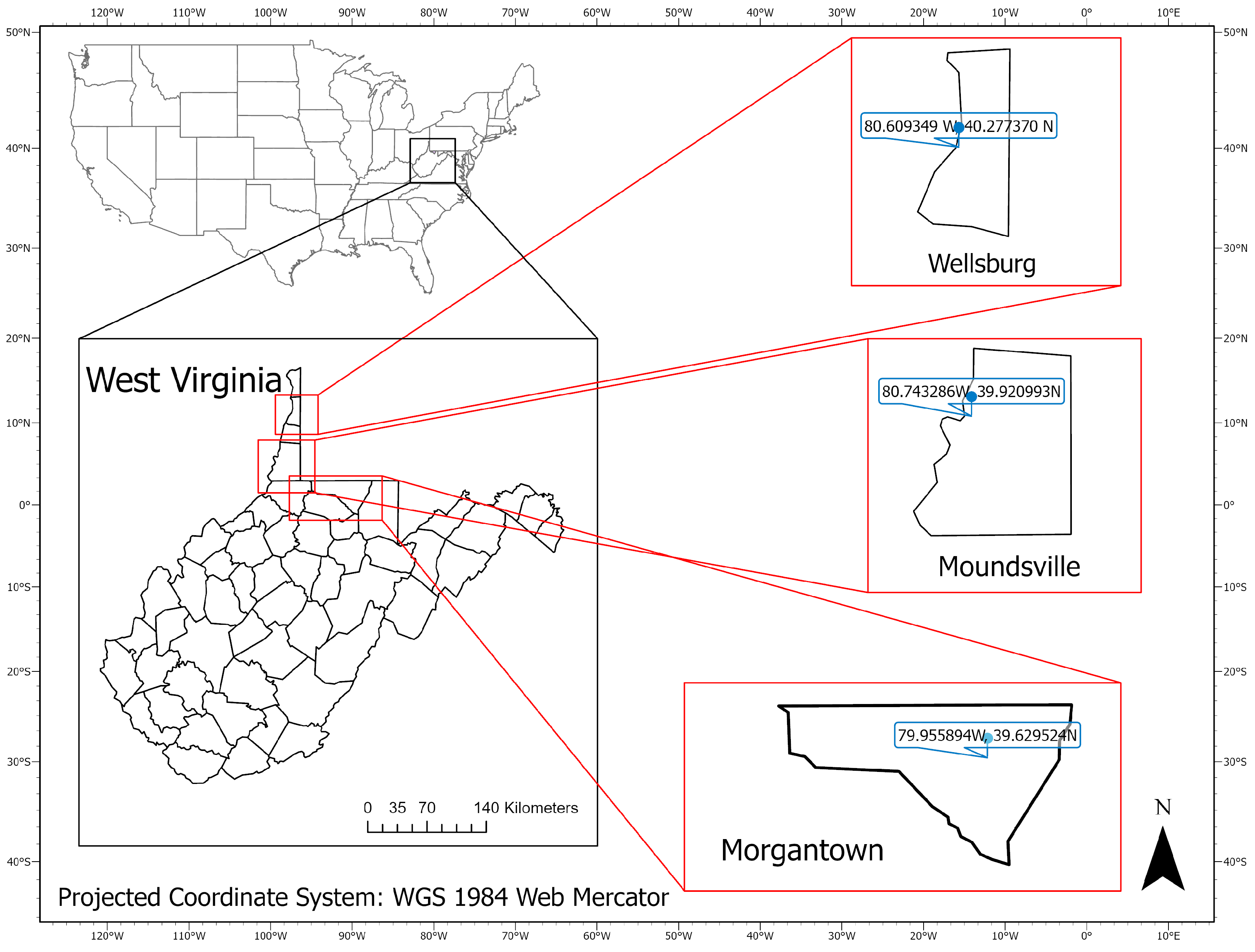
This study was conducted in three sentinel plots located in West Virginia, USA (Figure 1): Morgantown (39.629524 N, 79.955894 W), Wellsburg (40.277370 N, 80.609349 W), and Moundsville (39.920993 N, 80.743286 W). In the Morgantown site, six patches of knotweeds were used including two patches on the West Virginia University Organic Research Farm and four patches alongside the Monongahela River. In the Moundsville and Wellsburg sites, 19 knotweed patches were surveyed along the Ohio River and railroad.
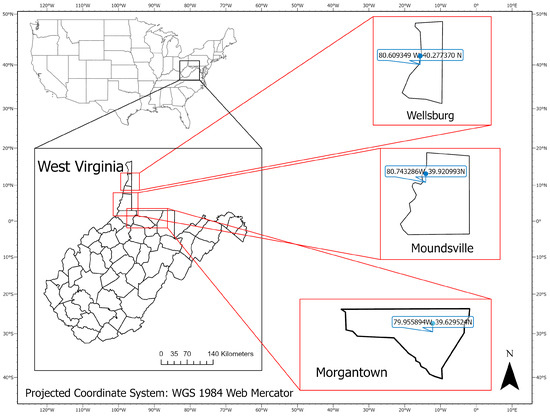
Figure 1.
Locations of three research sites: Morgantown, Wellsburg, and Moundsville, West Virginia, USA.
2.2. Aerial Surveys with Drones and Sensors
A total of 25 knotweed patches in the three sentinel plots were used for aerial surveys. We conducted six aerial surveys in April, June, August, September, and October of 2022–2024 to determine the optimal height of drone flight for detecting Japanese and giant knotweeds during their vegetative and flowering stages (Figure 2). Additionally, one survey was conducted in February 2024 to assess the feasibility of detecting knotweed patches in winter when they have no leaves. Japanese knotweed was dominant in all study sites while giant knotweed had a lesser prevalence (ca. 20% of all knotweed infestations). Bohemian knotweeds were rare, and Himalayan knotweeds were not found in our study sites, and thus they were not included in this study.

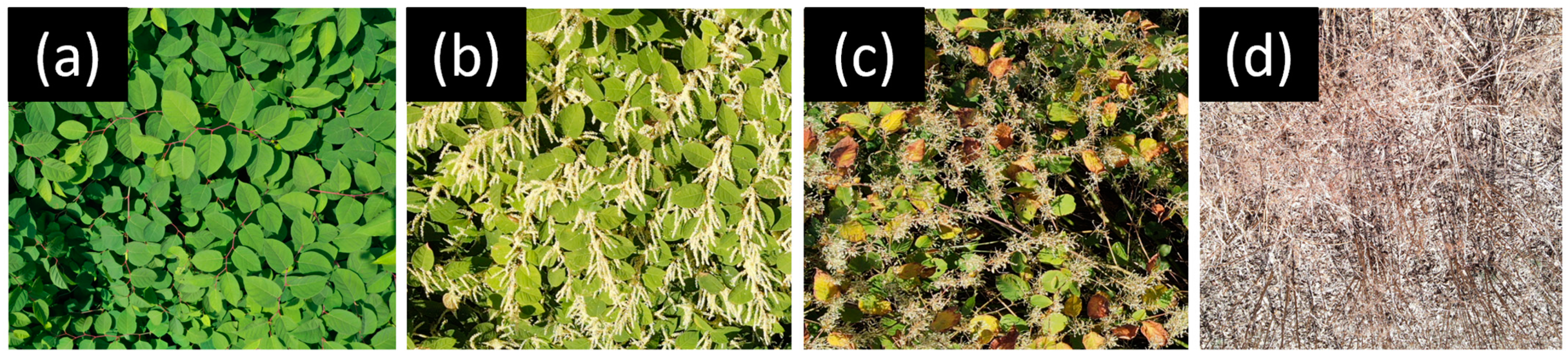
Figure 2.
Key morphological characteristics of leaf shape and arrangement, zigzag-shaped reddish stems of Japanese knotweed at the vegetative stage (a), creamy-white flowers (b), and creamy-white seed clusters (c) at the reproductive stage, and bare bamboo-like stems at the senescence stage (d). All the aerial images were taken at 5 m above the canopy.
We used DJI Mavic 2 Enterprise Advanced (SZ DJI Technology Co., Ltd., Shenzhen, China), which carries an RGB sensor with a 48-megapixel resolution. All drone flights in this study were conducted between noon and 3 PM on sunny days with a wind speed of <10 kph. The drone was flown at 16 different altitudes ranging from 5 m to 80 m above the canopy of the selected knotweed patches and images were taken every 5 m. After the aerial surveys were completed, the aerial images were downloaded from the drone.
Aerial images taken from different altitudes were visually examined to evaluate the detectability of knotweed leaves, inflorescences, and seed clusters. Japanese and giant knotweeds were identified based on their key morphological characteristics including leaf shape, alternate leaf arrangements, and zigzag-shaped stems (Figure 2a,b). Both Japanese and giant knotweeds have creamy-white flowers that emerge from where leaves meet the stem. The detectability was recorded as detectable (value = 1) at each flight altitude when our visual inspection of the aerial image could confirm key morphological characteristics of knotweeds. When we were unable to identify the features, detectability was recorded as undetectable (value = 0) [30]. The optimal flight height for detecting knotweeds was determined by analyzing the correlation between the detectability of knotweeds and flight heights. Logistic regression was used to analyze the data using R (v. 4.1.2, R Core Team, https://www.R-project.org (accessed on 1 February 2024)), library glmmTMB. Flight height above the canopy was used as the predictor, and the detectability at each altitude was recorded as a dependent variable. The chi-square values were used to evaluate the performance of the regression model for each growing stage.
In addition to RGB sensors, we acquired thermal images by using a 3.3-megapixel thermal camera measuring 8–14 µm with a 640 × 512 resolution carried by the DJI Mavic 2 Enterprise Advanced. The thermal images were taken 20 m above the canopy and analyzed using DJI Thermal Analysis Tool 3 (SZ DJI Technology Co., Ltd., Shenzhen, China). The average canopy temperature was measured for 10 randomly selected areas within patches of Japanese and giant knotweeds at the vegetative and flowering stages. RGB images carried by the same drone were used as the reference to locate the 10 selected areas in the thermal image. The values were compared with the average temperature of the surrounding vegetation shown on the thermal image. In addition, we used DJI Phantom 3 Advanced (SZ DJI Technology Co., Ltd., Shenzhen, China) that carried a multispectral sensor (Sentera, St. Paul, MN, USA). The sensors measured light reflectance of the red band: (625 nm) and near infrared band (850 nm). The bands from the multispectral sensor were separated and using the reflectance values of red and near-infrared wavelengths, normalized difference vegetative index (NDVI) was calculated by using a raster calculator in ArcGIS Pro (ESRI, Redland, CA, USA) for knotweeds and surrounding vegetation. RGB images were used as the reference to locate the 10 selected areas in NDVI images. Two sample t-tests using R were conducted to check the statistical significance between the thermal and NDVI values for the knotweed and the surrounding vegetation.
2.3. Development of Deep Learning Capability for Automated Identification
2.3.1. Aerial Surveys Using Drones
Aerial surveys to obtain aerial image data for deep learning were conducted over a 2-ha area within each of the three study sites. DJI Mavic 2 Enterprise Advanced which carries an RGB sensor with 4K videography capability was used for surveys. The drone was flown in a single transect along the railroad and trails with knotweed infestations. Aerial 4K videos were recorded 10–20 m above the canopy at vegetative and flowering stages of Japanese and giant knotweeds. Our preliminary flights showed that knotweeds were detectable at ≤20 m above the canopy. After the flight missions were completed, aerial images were downloaded from the drone and preprocessed for use in deep-learning models.
2.3.2. Data Preprocessing
The dataset used in this study was created from high-resolution 4K videos capturing sites containing various knotweed species. To ensure diversity and comprehensiveness, frames were extracted from the videos at regular intervals, specifically every 50th frame. Each extracted image was then divided into smaller 256 × 256 patches. This led to an increase in the size of the dataset and also mitigated the potential for overfitting by presenting the model with a wider range of spatial information. Furthermore, meticulous annotation was performed on each patch to assign it to one of the three target classes: giant knotweed at the vegetative stage, Japanese knotweed at the vegetative stage, or knotweeds at the flowering stage. Annotating each class with precision was imperative, considering scenarios where multiple species coexist within the same frame. To ensure accuracy, we carefully performed all annotations manually. Strict measures were implemented to guarantee that each annotated image contained only one knotweed species and no other plant species or background objects. This step was crucial for maintaining the integrity and consistency of the dataset and avoiding ambiguity during model training and evaluation. Additionally, a stratified split with a ratio of 7:2:1 for training, validation, and testing was employed for each class to ensure a representative distribution across the dataset subsets (Table 1).

Table 1.
Details of image distribution and dataset partitioning across knotweed species categories.
2.3.3. Overview of Swin Transformer
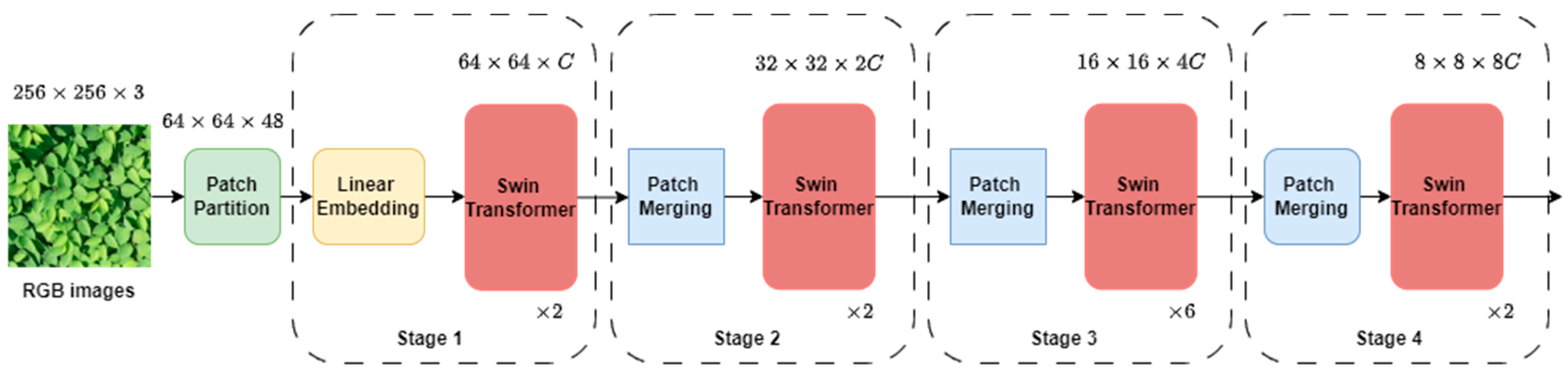
The methodology employed in this study leveraged the Swin Transformer architecture [29] for image classification tasks. The input RGB image was split into non-overlapping patches, with a patch size of 4, yielding feature dimensions of each patch as 4 × 4 × 3 = 48. We employed the tiny variant of the Swin Transformer. The overall network architecture is shown in Figure 3. Each raw feature dimension of the patches was passed through a linear embedding layer to project them to the arbitrary dimension ( = 96 in our study) and each patch passed through 4 stages (Figure 3). Each stage consisted of a Swin Transformer block which is a Transformer with modified self-attention. In Stage 1 of the Swin Transformer architecture, the Transformer blocks maintained a fixed number of tokens, defined as H/4 × W/4, where H and W represent the height and width of the input image, respectively. These tokens, along with the linear embedding, constituted the foundational components of stage 1. In Stage 2, as the network progresses deeper, a hierarchical representation is created by reducing the number of patches using patch merging layers. This method involved merging features from adjacent 2 × 2 patches and subsequently applying a linear layer to the combined features, resulting in a dimension of 4 . Therefore, there was a down-sampling of the resolution by a factor of 2 × 2 = 4, with the output dimension becoming 2 , while the resolution remained at H/8 × W/8. In Stage 3 and Stage 4, the procedure was iterated twice, resulting in output resolutions of H/16 × W/16 and H/32 × W/32, respectively.

Figure 3.
Swin Transformer network architecture: illustration of the Swin Transformer architecture utilized in the study, showcasing the stages and operations involved in processing input RGB images for classification tasks.
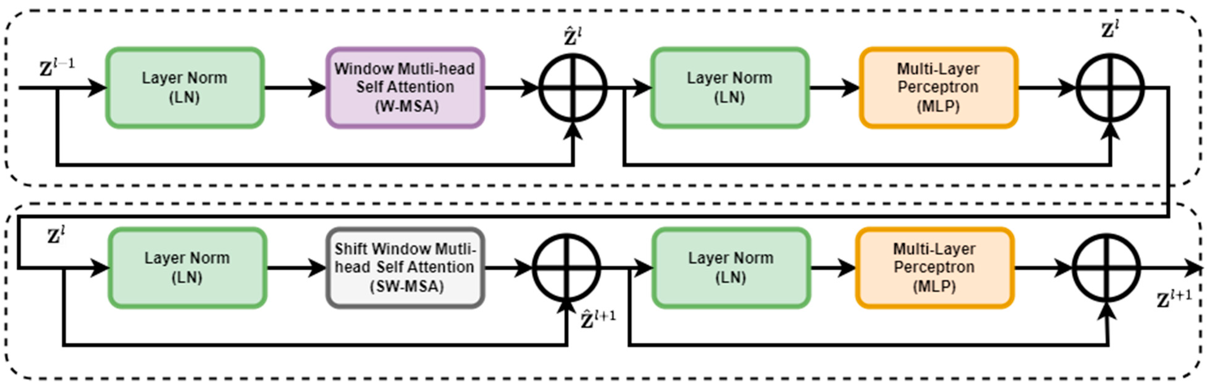
The Swin Transformer block replaced the standard multi-head self-attention (MSA) module in a Transformer block with a module based on shifted windows while keeping other layers unchanged. This block consisted of a shifted window-based MSA module, which handled attention mechanisms, followed by a 2-layer multi-layer perceptron (MLP) [31] with Gaussian error linear units (GELUs) [31] nonlinearity in between. LayerNorm (LN) layers were applied before each MSA module and MLP, and residual connections were applied after each module. The architecture of the Swin Transformer is shown in Figure 4.
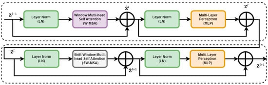
Figure 4.
Enhanced feature extraction with two successive Swin Transformer blocks.
The standard Transformer [26] architecture and its adaptation for image classification utilized global self-attention, resulting in quadratic complexity concerning the number of patches (Equation (1)). To address this, the methodology employed self-attention within local windows, dividing the image into non-overlapping windows. Each window comprises × patches ( = 7 throughout the study), with computational complexity evaluated specifically for the window-based self-attention (Equation (2)), highlighting its scalability for large numbers of patches.
where h and w are the height and width of the patch, respectively, is the embedding dimension set to 96, and is the size of the window set to 7. The Swin Transformer employed shifted window partitioning to enhance modeling without sacrificing computational efficiency. This method alternated between standard and shifted window configurations, facilitating inter-window connections. In consecutive blocks, output features were computed using Equation (3):
where and represented features from and modules, respectively. and denoted window-based multi-head self-attention with regular and shifted window partitioning, enabling connections between neighboring windows in the previous layer.
Swin Transformer’s shifted window partitioning technique increased the number of windows, potentially resulting in smaller window sizes. To handle this efficiently, a batch computation approach was proposed. Instead of padding smaller windows to × and masking padded values, a more efficient method was devised. This method cyclically shifted windows towards the top-left direction while maintaining the number of batched windows, ensuring computational efficiency. Finally, to calculate the self-attention, a relative position bias matrix B [32] was incorporated into each head to assess similarity (Equation (4)).
where , , and were matrices representing query, key, and value, respectively, with dimensions.
2.3.4. Data Augmentation and Training
Throughout our study, we employed the Swin Transformer’s tiny variant as our backbone to perform the classification of knotweed species. We utilized a dropout rate of 0.2, indicating that 20% of the units in the Swin Transformer backbone layer were randomly set to zero during training. This helped prevent the model from relying too heavily on specific features and encouraged it to learn more robust and generalizable representations. This regularization technique prevented overfitting, especially with limited training samples. The global average pooling layer (neck) was employed to aggregate spatial information across the feature maps generated by the backbone. This pooling operation computed the average value of each feature map channel, condensing spatial information into a single value per channel. A linear classifier head was chosen to produce class predictions based on the features extracted by the backbone and condensed by the neck. The head received input from 768 (4 × 4 × 16) channels, indicating the dimensionality of the feature representation produced by the backbone. Additionally, the label smooth loss with a smoothing value of 0.1 was employed to prevent overfitting by smoothing the one-hot encoded target labels, encouraging the model to generalize better.
where represents the label smoothing value (0.1). The cross-entropy () loss is the standard cross-entropy loss. Smoothed cross-entropy loss is the smoothed version of the cross-entropy loss, where instead of using one-hot encoded labels, each true label is replaced with a smoothed distribution over all classes. This smoothed distribution assigns a probability of to each non-true class and 1 − probability to the true class.
We also employed two augmentation techniques: Mixup [33] and CutMix [34], with each assigned specific α (degree of interpolation) values to regulate their impact. Mixup (α = 0.8) facilitated the blending of image pairs and their corresponding labels, thereby generating synthetic training samples that interpolated between the original samples in the input space. Conversely, CutMix (α = 1.0) orchestrated the cutting and pasting of patches from one image onto another, effectively amalgamating pixel values and labels from disparate images. We selected α values based on recommendations from two studies [33,34], which balanced the trade-off between data augmentation and label smoothing. Mixup blended image pairs and their labels to generate synthetic samples, while CutMix combined patches from different images. Preliminary experiments showed these techniques improved training stability and performance for our dataset. The primary goal was to enhance the robustness of the training process rather than to improve accuracy only. Mixup and CutMix introduced variability, helping the model generalize better and prevent overfitting. In addition to data augmentation, we incorporated data preprocessing operations such as random resized cropping, flipping, random augmentation, and random erasing. AdamW was employed as the optimizer with a learning rate of 0.001. Weight decay was set to 0.05, epsilon to 1 × 10⁻⁸, and betas to (0.9, 0.999). The learning policy involved linear learning rate warm-up for the first 20 epochs, transitioning to cosine annealing with a minimum learning rate of 1 × 10⁻⁵ after epoch 20. The training configuration was defined with a maximum of 300 epochs with validation performed at each epoch. Additionally, the learning rate could be dynamically scaled based on the actual training batch size using the automatic scaling of the learning rate mechanism, with a base batch size of 128. All experiments were conducted on a single NVIDIA GeForce RTX 3090 GPU. Other environment details include Python 3.10.12, GCC 11.4.0, CUDA 11.8, PyTorch version 2.3.0 with CUDA toolkit compatibility version 11.2.1, MMPretrain 1.2.0 [35], CuDNN 8.9.2, and Ubuntu 22.04.
3. Results
3.1. Detection of Knotweeds Using Aerial Imagery
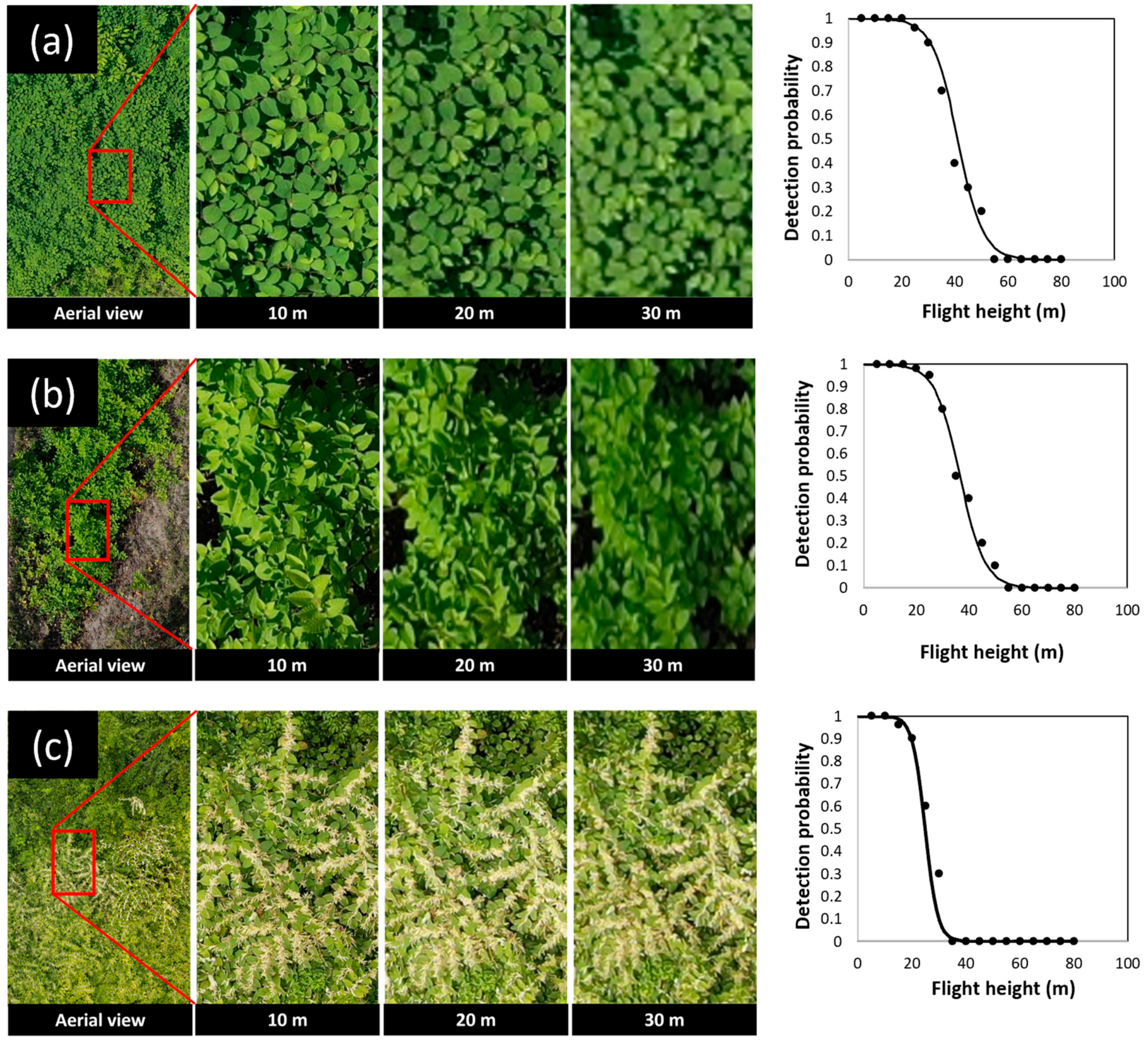
The morphological characteristics, including leaf shape, alternate leaf arrangements, and zigzag-shaped stems of knotweeds, were detectable on RGB images taken by drone in April and June. The relationship between flight height and detectability of Japanese knotweed at the vegetative stage fitted best with logistic regression (χ2 = 30.725, df = 1, p < 0.0001). The results of regression analysis showed that at early and full vegetative stages in April and June, Japanese knotweed was detectable up to 50 m above the canopy. The probability of detection was 100% at ≤35 m above the canopy (Figure 5). At higher flight heights, individual branches located on the margin of the Japanese knotweed patches were readily detectable compared to those located in the center of the patch.

Figure 5.
Example aerial images (RGB) of knotweeds at different flight heights above the canopy and their relationship with the probability of detecting Japanese knotweed (a), giant knotweed (b) at the vegetative stage, and Japanese knotweed at flowering stage (c).
Giant knotweed was also detectable up to 50 m while the probability of detection was 100% at ≤25 m above the canopy (Figure 5). At higher flight heights, the lower resolution of images made the heart-shaped leaf base of giant knotweed not apparent and, thus, visual detection of this species became very challenging. The relationship between flight height and detectability of giant knotweed at the vegetative stage fitted best with logistic regression (χ2 = 15.166, df = 1, p < 0.0001).
Flowers and seed clusters of Japanese and giant knotweeds were detectable on RGB images taken by drone in August, September, and October. The relationship between flight height and detectability of knotweeds at the flowering and seeding stage fitted best with logistic regression (χ2 = 16.62, df = 1, p < 0.0001). The results of regression analysis showed that, at this stage, knotweeds were detectable up to 30 m above the canopy and that the probability of detection was 100% at ≤20 m above the canopy (Figure 5). We found that knotweeds were not detectable on aerial images during winter when the bare bamboo-like stems were the only part of the plants left on the ground (Figure 2d).
There was no significant difference between the temperature and NDVI values of the knotweeds and those of other surrounding vegetation (Figure S1 from Supplementary Materials). The thermal image showed no statistically significant difference for the Japanese knotweed at both the vegetative and flowering stages and for giant knotweed at the vegetative stage with the surrounding vegetation (Table 2). Also, no significant differences in the NDVI values between knotweeds and surrounding plants were found. The NDVI value for Japanese knotweed was 0.89 ± 0.05 while NDVI values for surrounding plants were 0.88 ± 0.06 for common buttonbush (t = 0.1811, df = 2, p = 0.8730), 0.91 ± 0.03 for red clover (t = 0.4851, df = 2, p = 0.6756), 0.90 ± 0.02 (t = 0.2626, df = 2, p = 0.8174) for orchard grass, and 0.91 ± 0.02 (t = 0.5252, df = 2, p = 0.6518) for water wisteria.
Table 2.
Comparison between temperatures in each knotweed species canopy and surrounding vegetation.
3.2. Deep Learning for Knotweed Classification
In our study, we conducted a comparative analysis of various CNNs and Transformers to classify knotweed species, evaluating single-label accuracy, precision, and recall. The empirical results (Table 3) indicated that Swin Transformer outperformed other methods in terms of accuracy, precision, and recall. Swin Transformer achieved superior performance compared to ViT-B, with an accuracy of 99.4758% (0.1686% higher), precision of 99.4713% (0.1768% higher), and recall of 99.483% (0.1585% higher). These empirical results demonstrate the superior performance of the Swin Transformer compared to both CNNs and other transformer architectures, highlighting its effectiveness in the classification task.
Table 3.
Comparison of state-of-the-art baselines and backbones for knotweed species classification.
3.2.1. Evaluation of the Deep Learning Model
During the training process, we monitored the performance metrics of accuracy, precision, recall, and loss across epochs to assess the convergence and effectiveness of our models (Figure 6). The plots for the Swin Transformer model, tasked with classifying three categories—giant knotweed at the vegetative stage, knotweed at the flowering stage, and Japanese knotweed at the vegetative stage—offered insightful glimpses into its performance dynamics. The accuracy plot (Figure 6a) revealed its overall classification proficiency, while precision (Figure 6b) and recall (Figure 6c) provided detailed perspectives on its ability to minimize false positives and false negatives, crucial given class imbalances. Moreover, the loss plot (Figure 6d) traced the model’s optimization journey, showcasing parameter convergence toward minimizing the loss function. These analyses provided a comprehensive understanding of the model’s training process, guiding informed decisions on fine-tuning strategies and model selection for effective classification.
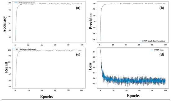
Figure 6.
Training performance metrics for knotweed classification with the Swin Transformer: accuracy (a), precision (b), recall (c), and loss (d) over epochs.
3.2.2. Confusion Matrix
The confusion matrix provides a detailed breakdown of the model’s classification performance across knotweed species. Our results showed the model achieved notable accuracy in predicting giant knotweed, with a classification rate of 95.64% (Table 4). Similarly, the model performed exceptionally well in identifying Japanese knotweed at the flowering and vegetative stages, achieving classification rates of 97.32% and 100%, respectively. These values signify instances where the predicted label matches the true label, demonstrating the model’s ability to differentiate between knotweed species accurately. Conversely, off-diagonal elements represent misclassifications, highlighting areas where the model may struggle to distinguish between specific classes. Analyzing these discrepancies can offer valuable insights for refining the model and improving its performance in practical applications. The evaluation was conducted on a distinct test dataset to assess the model’s predictive efficacy. What is noteworthy is the occurrence of misclassifications, notably, instances where giant knotweed at the vegetative stage was erroneously identified as Japanese knotweed at the flowering stage, and vice versa (see Figure S2 from Supplementary Materials for example). These misclassifications underscore the inherent complexities in automated species differentiation, particularly when dealing with visually similar features. Such misclassifications provide valuable insights into the challenges associated with fine-grained classification tasks within the domain of computer vision and deep learning.
Table 4.
The confusion matrix visualizes the classification performance of the model across different classes: giant knotweed at the vegetative stage, knotweeds at the flowering stage, and Japanese knotweed at the vegetative stage. Each row corresponds to instances from the actual (true) class, while each column represents predictions made by the model for a specific class. The diagonal elements of the matrix indicate the number of accurately classified instances within each class.
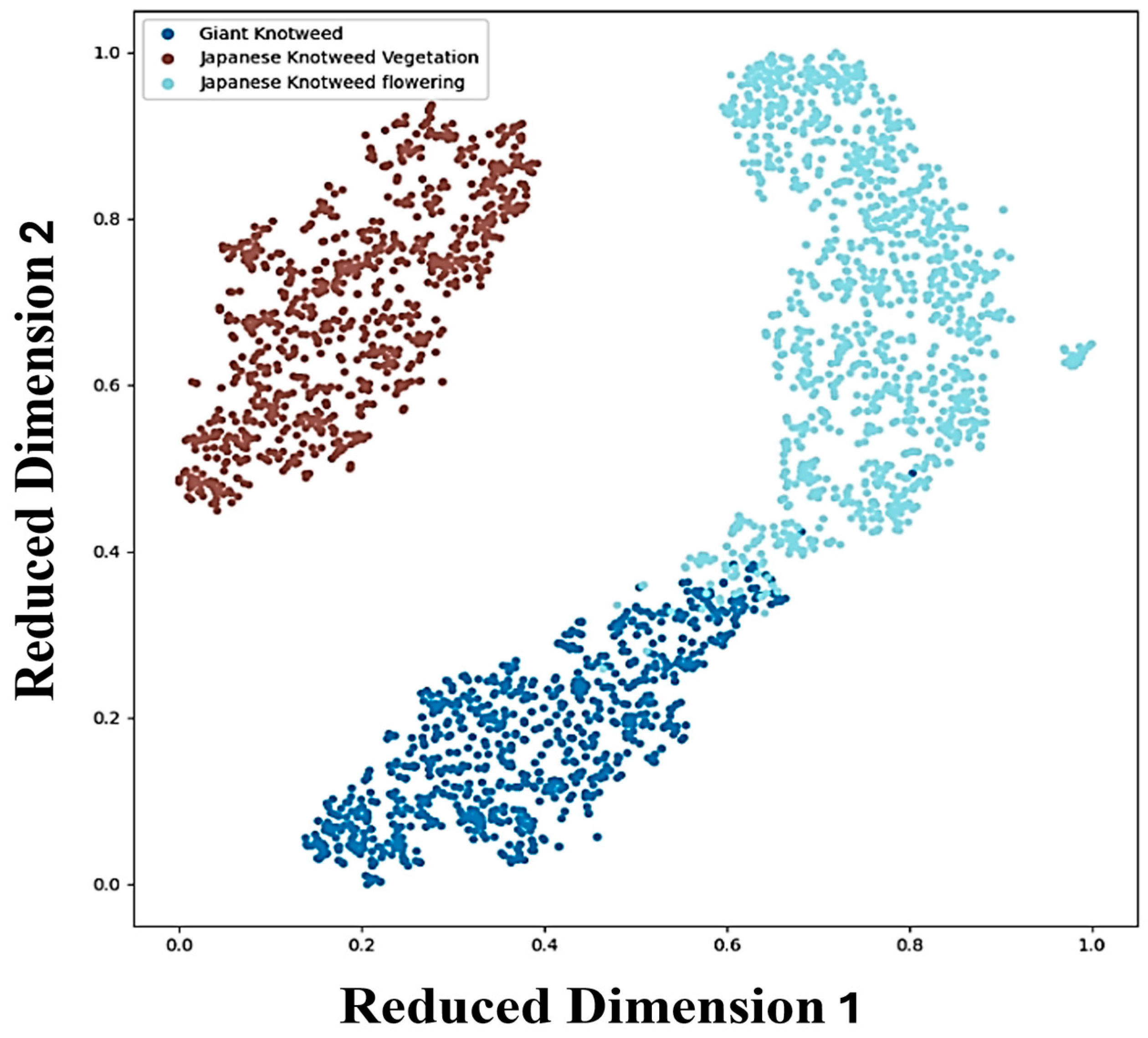
We generated a t-SNE plot (Figure 7) [36] to visualize our knotweed species dataset, illustrating the relationships between different species based on their reduced-dimensional features. Each point on the plot represents the extracted features from knotweed image patches, showcasing distinct clusters corresponding to separate species classes. While separate clusters indicate clear distinctions between species, overlaps between clusters, particularly observed between giant knotweed and Japanese knotweed at the flowering stage, suggest shared characteristics or similarities. This overlap underscores the challenges in accurately distinguishing between closely related species based solely on the extracted features. Variations within clusters might arise from diverse factors, including environmental conditions, growth stages, genetic diversity, and patch variation such as uneven or slightly different growth stages of knotweeds and light conditions affecting drone sensors.
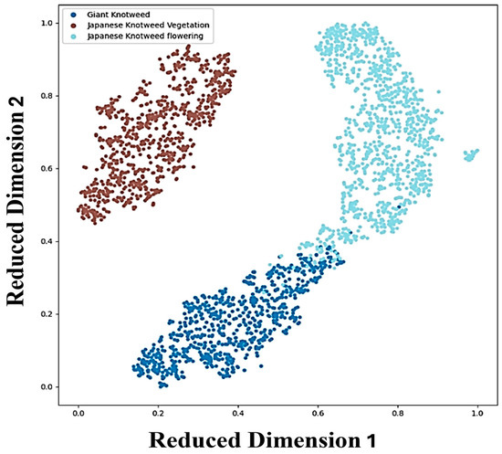
Figure 7.
t-SNE visualization of feature extraction from Swin Transformer for the classification of giant and Japanese knotweeds at the vegetative stage and knotweeds at the flowering stage. The x- and y-axes of the t-SNE plot represent the reduced-dimensional space of the knotweed species dataset, ranging from 0 to 1 to facilitate comparison and visualization of extracted characteristics from the image patches.
4. Discussion
Overall, our findings suggest that identifying knotweeds on aerial images is more achievable during the vegetative stage compared to the flowering or seeding stage. This is because the distinctive leaf shape and zigzag pattern of the stems are more discernible during the vegetative stage. However, knotweed flower clusters emerge from where leaves meet the stem and cover the leaf base and zigzag-shaped stem, making detection more difficult, particularly on aerial images taken at higher flight heights. Color changes, senescence of leaves, and falling petals made it difficult to detect key knotweed morphological characteristics of knotweed species at higher flight heights, especially in the fall. However, this may not affect the current knotweed management because the detection of knotweed patches and the implementation of control measures are generally done before knotweeds reach full vegetative or flowering stages. The results of this study also highlight that the optimum flight height for detecting giant knotweed at the vegetative stage using drones was lower than that for detecting Japanese knotweed. We used a leaf base for identifying the two knotweed species at the vegetative stage. Unlike the flat leaf base of Japanese knotweed, which was detectable up to 35 m with 100% probability, the heart-shaped leaf base of giant knotweed was not 100% detectable at >25 m above the canopy.
Our study clearly demonstrated that drones equipped with an RGB sensor can be used for the detection and identification of invasive knotweed species. Typical drone flights over agricultural lands or forests could be conducted with a small crew, covering large areas in a short amount of time, making drones an attractive tool for invasive plant detection and management. Furthermore, the flexibility of the drone and the modularity of the onboard payload allow for easy retrofits with a wide range of high-resolution imaging payloads. With the implementation of an onboard control system, drone flights could be tailored to meet site-specific monitoring strategies because they can be programmed to cover specific areas that need additional or repeated monitoring. Knotweeds usually inhabit near waterways where chemical control is limited, impractical, and harmful to the aquatic ecosystem with caution considerations required [37]. Aerial releases of natural enemies to control invasive weeds have been successfully tested using drones [38]. Currently, the knotweed psyllid (Aphalara itadori), a natural enemy of Japanese knotweed, is available [39] and thus developing an aerial release method for biological control of knotweed would lead to the possibility of spatially targeted management, particularly in inaccessible areas where ground-based management is difficult or chemical control is limited.
Incorporating AI and deep learning for multi-class classification presents several noteworthy advantages, as demonstrated in our study. It is essential to acknowledge the various approaches employed in similar studies for classifying crops using remote sensing datasets [40,41,42], including thermal [43,44,45], multispectral, and multitemporal [46,47] images. However, since knotweed cannot be reliably identified using thermal or multispectral imagery, we opted to focus our deep learning analysis solely on RGB images. By utilizing images and videos captured by drones and employing deep learning for classification, we gain the ability to access remote or challenging terrains where human accessibility is limited, if not impossible. This capability significantly expands the scope of ecological monitoring and forest health management, enabling us to gather vital data from areas previously inaccessible. Additionally, the automation facilitated by deep learning models makes the process highly cost-effective, as it reduces the need for manual labor and extensive fieldwork. Moreover, employing state-of-the-art deep learning models ensures high accuracy and reliability in species classification, enhancing the overall effectiveness of ecological monitoring efforts. However, it is essential to acknowledge certain limitations and challenges encountered during our study. One notable issue is the potential for misclassification, particularly regarding distinguishing between giant knotweed and Japanese knotweed flowering. This challenge arises due to similarities in appearance, such as flower morphology, which can lead to misinterpretation, especially when images lack complete foliage for reference. Furthermore, our dataset primarily focuses on knotweed species without considering background noise or the presence of other plant species, potentially limiting the model’s generalizability to more diverse ecological settings. Additionally, although we ensured that each annotated image contains only one instance of giant knotweed, the coexistence of multiple knotweed species within the same frame may pose challenges to the model’s accuracy. In addition, the model’s performance under different environmental conditions and with various types of background interference is critical. Evaluating these factors is essential to improve the robustness and generalizability of the Swin Transformer in real-world invasive plant monitoring and vegetation classification scenarios. This includes assessing the Transformer’s ability to accurately classify species amidst diverse and dynamic environmental contexts, as well as its resilience to varying levels of background noise.
To address these limitations and enhance the robustness of our classification system, future research should explore innovative approaches involving the adaptation of per-pixel classification techniques, such as segmentation [48,49] or object recognition [50], to achieve finer-grained species identification. By analyzing individual pixels within an image, we can more accurately delineate between different plant species, even in complex and overlapping scenarios. Additionally, flying drones at higher flight heights or using high-resolution sensors offers several advantages, including mitigating data loss caused by leaf folding due to lower drone flight. This strategic approach not only enhances data collection efficiency but also minimizes the risk of misclassification by capturing clearer and more comprehensive aerial imagery. Overall, these proposed advancements hold significant promise for advancing the field of ecological monitoring and vegetation classification using AI-driven drone technology.
5. Conclusions
This study reports that Japanese knotweed and giant knotweed at their vegetative stage were detectable at ≤35 m and ≤25 m, respectively, above the canopy using an RGB sensor. The flowers of the knotweeds were detectable at ≤20 m. Swin Transformer achieved high precision, recall, and accuracy in automated knotweed detection on aerial images acquired with drones and RGB sensors. The results of this study provide three important implications for knotweed detection and management. Firstly, aerial surveys can accelerate and facilitate detecting knotweed hotspots and monitoring invaded habitats compared to laborious and time-consuming ground surveys. Secondly, automated detection and mapping of knotweed patches and hotspots can be used for site-specific management of knotweeds and planning and prioritizing different control measures (e.g., mechanical, chemical, or biological control). Lastly, employing automated detection with machine learning capabilities opens up new possibilities for knotweed management. Through the integration of the Internet of Things (IoT), it becomes feasible to conduct real-time monitoring and apply herbicides using drones.
Supplementary Materials
The following supporting information can be downloaded at: https://www.mdpi.com/article/10.3390/drones8070293/s1, Figure S1: Example aerial images of Japanese knotweed taken with different optical sensors: RGB (a), thermal (b), and NDVI values from a multispectral sensor (c). The whiter color in (b) indicates higher temperature and the greener color in (c) indicates healthy vegetation. Figure S2: Example outcomes of knotweed species classification utilizing the Swin Transformer model.
Author Contributions
Conceptualization, R.K. and Y.-L.P.; methodology, R.K., Y.-L.P., S.K.V. and K.N.; software, R.K., S.K.V. and K.N.; validation, R.K. and S.K.V.; formal analysis, R.K., S.K.V. and K.N.; investigation, R.K., Y.-L.P., S.K.V. and K.N.; resources, Y.-L.P. and X.L.; data curation, R.K. and S.K.V.; writing—original draft preparation, R.K., S.K.V. and K.N.; writing—review and editing, R.K., Y.-L.P., X.L., S.K.V. and K.N.; visualization, R.K., S.K.V. and K.N.; supervision, Y.-L.P. and X.L.; project administration, Y.-L.P. and X.L.; funding acquisition, Y.-L.P. and X.L. All authors have read and agreed to the published version of the manuscript.
Funding
This research was supported by the USDA NIFA AFRI Foundational and Applied Sciences Grant Program (2021-67014-33757) and the West Virginia Agriculture and Forestry Experiment Station Hatch Project (WVA00785).
Data Availability Statement
Data will be available upon request.
Acknowledgments
We would like to thank Cynthia Huebner at the USDA Forest Service for her help with the identification of knotweed species and for her valuable comments on the study.
Conflicts of Interest
The authors declare no conflicts of interest.
References
- Wilson, L.M. Key to Identification of Invasive Knotweeds in British Columbia; Ministry of Forests and Range, Forest Practices Branch: Kamloops, BC, Canada, 2007. [Google Scholar]
- Parkinson, H.; Mangold, J. Biology, Ecology and Management of the Knotweed Complex; Montana State University Extension: Bozeman, MT, USA, 2010. [Google Scholar]
- Brousseau, P.-M.; Chauvat, M.; De Almeida, T.; Forey, E. Invasive knotweed modifies predator–prey interactions in the soil food web. Biol. Invasions 2021, 23, 1987–2002. [Google Scholar] [CrossRef]
- Kato-Noguchi, H. Allelopathy of knotweeds as invasive plants. Plants 2021, 11, 3. [Google Scholar] [CrossRef] [PubMed]
- Colleran, B.; Lacy, S.N.; Retamal, M.R. Invasive Japanese knotweed (Reynoutria japonica Houtt.) and related knotweeds as catalysts for streambank erosion. River Res. Appl. 2020, 36, 1962–1969. [Google Scholar] [CrossRef]
- Payne, T.; Hoxley, M. Identifying and eradicating Japanese knotweed in the UK built environment. Struct. Surv. 2012, 30, 24–42. [Google Scholar] [CrossRef]
- Dusz, M.-A.; Martin, F.-M.; Dommanget, F.; Petit, A.; Dechaume-Moncharmont, C.; Evette, A. Review of existing knowledge and practices of tarping for the control of invasive knotweeds. Plants 2021, 10, 2152. [Google Scholar] [CrossRef]
- Rejmánek, M.; Pitcairn, M.J. When is eradication of exotic plant pests a realistic goal? In Turning the Tide: The Eradication of Invasive Species, Proceedings of the International Conference on Eradication of Island Invasives, Auckland, New Zealand, 19–23 February 2001; Veitch, C.R., Clout, M.N., Eds.; IUCN SSC Invasive Species Specialist Group: Gland, Switzerland; Cambridge, UK, 2002; 414p. [Google Scholar]
- Hocking, S.; Toop, T.; Jones, D.; Graham, I.; Eastwood, D. Assessing the relative impacts and economic costs of Japanese knotweed management methods. Sci. Rep. 2023, 13, 3872. [Google Scholar] [CrossRef] [PubMed]
- Shahi, T.B.; Dahal, S.; Sitaula, C.; Neupane, A.; Guo, W. Deep learning-based weed detection using UAV images: A comparative study. Drones 2023, 7, 624. [Google Scholar] [CrossRef]
- López-Granados, F. Weed detection for site-specific weed management: Mapping and real-time approaches. Weed Res. 2011, 51, 1–11. [Google Scholar] [CrossRef]
- Hasan, A.S.M.M.; Sohel, F.; Diepeveen, D.; Laga, H.; Jones, M.G. A survey of deep learning techniques for weed detection from images. Comput. Electron. Agric. 2021, 184, 106067. [Google Scholar]
- Lambert, J.P.T.; Hicks, H.L.; Childs, D.Z.; Freckleton, R.P. Evaluating the potential of unmanned aerial systems for mapping weeds at field scales: A case study with Alopecurus myosuroides. Weed Res. 2018, 58, 35–45. [Google Scholar] [CrossRef]
- Singh, V.; Rana, A.; Bishop, M.; Filippi, A.M.; Cope, D.; Rajan, N.; Bagavathiannan, M. Unmanned aircraft systems for precision weed detection and management: Prospects and challenges. Adv. Agron. 2020, 159, 93–134. [Google Scholar]
- Barbizan Sühs, R.; Ziller, S.R.; Dechoum, M. Is the use of drones cost-effective and efficient in detecting invasive alien trees? A case study from a subtropical coastal ecosystem. Biol. Invasions 2024, 26, 357–363. [Google Scholar] [CrossRef]
- Bradley, B.A. Remote detection of invasive plants: A review of spectral, textural and phenological approaches. Biol. Invasions 2014, 16, 1411–1425. [Google Scholar] [CrossRef]
- Lass, L.W.; Prather, T.S.; Glenn, N.F.; Weber, K.T.; Mundt, J.T.; Pettingill, J. A review of remote sensing of invasive weeds and example of the early detection of spotted knapweed (Centaurea maculosa) and baby’s breath (Gypsophila paniculata) with a hyperspectral sensor. Weed Sci. 2005, 53, 242–251. [Google Scholar] [CrossRef]
- Miotto, R.; Wang, F.; Wang, S.; Jiang, X.; Dudley, J.T. Deep learning for healthcare: Review, opportunities and challenges. Brief. Bioinform. 2018, 19, 1236–1246. [Google Scholar] [CrossRef] [PubMed]
- Zhu, X.X.; Tuia, D.; Mou, L.; Xia, G.S.; Zhang, L.; Xu, F.; Fraundorfer, F. Deep learning in remote sensing: A comprehensive review and list of resources. IEEE Geosci. Remote Sens. Mag. 2017, 5, 8–36. [Google Scholar] [CrossRef]
- Zhang, Y.; Yan, J.; Chen, S.; Gong, M.; Gao, D.; Zhu, M.; Gan, W. Review of the applications of deep learning in bioinformatics. Curr. Bioinform. 2020, 15, 898–911. [Google Scholar] [CrossRef]
- Otter, D.W.; Medina, J.R.; Kalita, J.K. A survey of the usages of deep learning for natural language processing. IEEE Trans. Neural Netw. Learn. Syst. 2020, 32, 604–624. [Google Scholar] [CrossRef] [PubMed]
- Simonyan, K. Very deep convolutional networks for large-scale image recognition. arXiv 2015. [Google Scholar] [CrossRef]
- He, K.; Zhang, X.; Ren, S.; Sun, J. Deep residual learning for image recognition. In Proceedings of the IEEE Conference on Computer Vision and Pattern Recognition, Las Vegas, NV, USA, 27–30 June 2016; IEEE: Piscataway, NJ, USA, 2016; pp. 770–778. [Google Scholar]
- Huang, G.; Liu, Z.; Van Der Maaten, L.; Weinberger, K.Q. Densely connected convolutional networks. In Proceedings of the IEEE Conference on Computer Vision and Pattern Recognition, Honolulu, HI, USA, 21–26 July 2017; IEEE: Piscataway, NJ, USA, 2017; pp. 4700–4708. [Google Scholar]
- Tan, M.; Le, Q. Efficientnet: Rethinking model scaling for convolutional neural networks. In Proceedings of the International Conference on Machine Learning, PMLR 97, Long Beach, CA, USA, 9–15 June 2019; pp. 6105–6114. [Google Scholar]
- Vaswani, A.; Shazeer, N.; Parmar, N.; Uszkoreit, J.; Jones, L.; Gomez, A.N.; Kaiser, Ł.; Polosukhin, I. Attention is all you need. In Proceedings of the Advances in Neural Information Processing Systems 2017, Long Beach, CA, USA, 4–9 December 2017; Volume 30. [Google Scholar]
- Dosovitskiy, A.; Beyer, L.; Kolesnikov, A.; Weissenborn, D.; Zhai, X.; Unterthiner, T.; Dehghani, M.; Minderer, M.; Heigold, G.; Gelly, S.; et al. An image is worth 16 × 16 words: Transformers for image recognition at scale. In Proceedings of the 9th International Conference on Learning Representations, ICLR 2021, Virtual, 3–7 May 2021. [Google Scholar]
- Touvron, H.; Cord, M.; Douze, M.; Massa, F.; Sablayrolles, A.; Jegou, H. Training data-efficient image transformers & distillation through attention. In Proceedings of the 38th International Conference on Machine Learning, PLMR 139, Virtual, 18–24 July 2021; pp. 10347–10357. [Google Scholar]
- Liu, Z.; Lin, Y.; Cao, Y.; Hu, H.; Wei, Y.; Zhang, Z.; Lin, S.; Guo, B. Swin transformer: Hierarchical vision transformer using shifted windows. In Proceedings of the IEEE/CVF International Conference on Computer Vision, Nashville, TN, USA, 20–25 June 2021; IEEE: Piscataway, NJ, USA, 2021; pp. 10012–10022. [Google Scholar]
- Naharki, K.; Huebner, C.D.; Park, Y.-L. The detection of tree of heaven (Ailanthus altissima) using drones and optical sensors: Implications for the management of invasive plants and insects. Drones 2023, 8, 1. [Google Scholar] [CrossRef]
- Haykin, S. Neural Networks: A Comprehensive Foundation; Prentice Hall PTR: Upper Saddle River, NJ, USA, 1998. [Google Scholar]
- Raffel, C.; Shazeer, N.; Roberts, A.; Lee, K.; Narang, S.; Matena, M.; Zhou, Y.; Li, W.; Liu, P.J. Exploring the limits of transfer learning with a unified text-to-text transformer. J. Mach. Learn. Res. 2020, 21, 1–67. [Google Scholar]
- Zhang, H.; Cisse, M.; Dauphin, Y.N.; Lopez-Paz, D. mixup: Beyond Empirical Risk Minimization. In Proceedings of the International Conference on Learning Representations, Vancouver, BC, Canada, 30 April–3 May 2018. [Google Scholar]
- Yun, S.; Han, D.; Oh, S.J.; Chun, S.; Choe, J.; Yoo, Y. Cutmix: Regularization strategy to train strong classifiers with localizable features. In Proceedings of the IEEE/CVF International Conference on Computer Vision, Seoul, Republic of Korea, 27 October–2 November 2019; IEEE: Piscataway, NJ, USA, 2019; pp. 6023–6032. [Google Scholar]
- MMPretrain Contributors. OpenMMLab’s Pre-Training Toolbox and Benchmark. 2023. Available online: https://github.com/open-mmlab/mmpretrain (accessed on 28 April 2024).
- Van der Maaten, L.; Hinton, G. Visualizing data using t-SNE. J. Mach. Learn. Res. 2008, 9, 2579–2605. [Google Scholar]
- Grevstad, F.S.; Andreas, J.E.; Bourchier, R.S.; Shaw, R.; Winston, R.L.; Randall, C.B. Biology and Biological Control of Knotweeds; United States Department of Agriculture, Forest Health Assessment and Applied Sciences Team: Fort Collins, CO, USA, 2018. [Google Scholar]
- Park, Y.L.; Gururajan, S.; Thistle, H.; Chandran, R.; Reardon, R. Aerial release of Rhinoncomimus latipes (Coleoptera: Curculionidae) to control Persicaria perfoliata (Polygonaceae) using an unmanned aerial system. Pest Manag. Sci. 2018, 74, 141–148. [Google Scholar] [CrossRef] [PubMed]
- Shaw, R.H.; Bryner, S.; Tanner, R. The life history and host range of the Japanese knotweed psyllid, Aphalara itadori Shinji: Potentially the first classical biological weed control agent for the European Union. Biol. Control 2009, 49, 105–113. [Google Scholar] [CrossRef]
- Kussul, N.; Lavreniuk, M.; Skakun, S.; Shelestov, A. Deep learning classification of land cover and crop types using remote sensing data. IEEE Geosci. Remote Sens. Lett. 2017, 14, 778–782. [Google Scholar] [CrossRef]
- Agilandeeswari, L.; Prabukumar, M.; Radhesyam, V.; Phaneendra, K.L.B.; Farhan, A. Crop classification for agricultural applications in hyperspectral remote sensing images. Appl. Sci. 2022, 12, 1670. [Google Scholar] [CrossRef]
- Orynbaikyzy, A.; Gessner, U.; Conrad, C. Crop type classification using a combination of optical and radar remote sensing data: A review. Int. J. Remote Sens. 2019, 40, 6553–6595. [Google Scholar] [CrossRef]
- Batchuluun, G.; Nam, S.H.; Park, K.R. Deep learning-based plant classification and crop disease classification by thermal camera. J. King Saud Univ.-Comput. Inf. Sci. 2022, 34, 10474–10486. [Google Scholar] [CrossRef]
- Barnes, M.L.; Yoder, L.; Khodaee, M. Detecting winter cover crops and crop residues in the Midwest US using machine learning classification of thermal and optical imagery. Remote Sens. 2021, 13, 1998. [Google Scholar] [CrossRef]
- Chandel, N.S.; Rajwade, Y.A.; Dubey, K.; Chandel, A.K.; Subeesh, A.; Tiwari, M.K. Water stress identification of winter wheat crop with state-of-the-art AI techniques and high-resolution thermal-RGB imagery. Plants 2022, 11, 3344. [Google Scholar] [CrossRef]
- Gadiraju, K.K.; Ramachandra, B.; Chen, Z.; Vatsavai, R.R. Multimodal deep learning-based crop classification using multispectral and multitemporal satellite imagery. In Proceedings of the 26th International Conference on Knowledge Discovery & Data Mining, Virtual, 6–10 July 2020; Association for Computing Machinery: New York, NY, USA, 2020; pp. 3234–3242. [Google Scholar]
- Siesto, G.; Fernández-Sellers, M.; Lozano-Tello, A. Crop classification of satellite imagery using synthetic multitemporal and multispectral images in convolutional neural networks. Remote Sens. 2021, 13, 3378. [Google Scholar] [CrossRef]
- Khan, S.D.; Basalamah, S.; Lbath, A. Weed–Crop segmentation in drone images with a novel encoder–decoder framework enhanced via attention modules. Remote Sens. 2023, 15, 5615. [Google Scholar] [CrossRef]
- Genze, N.; Wirth, M.; Schreiner, C.; Ajekwe, R.; Grieb, M.; Grimm, D.G. Improved weed segmentation in UAV imagery of sorghum fields with a combined deblurring segmentation model. Plant Methods 2023, 19, 87. [Google Scholar] [CrossRef]
- Valicharla, S.K.; Li, X.; Greenleaf, J.; Turcotte, R.; Hayes, C.; Park, Y.-L. Precision detection and assessment of ash death and decline caused by the emerald ash borer using drones and deep learning. Plants 2023, 12, 798. [Google Scholar] [CrossRef]

Disclaimer/Publisher’s Note: The statements, opinions and data contained in all publications are solely those of the individual author(s) and contributor(s) and not of MDPI and/or the editor(s). MDPI and/or the editor(s) disclaim responsibility for any injury to people or property resulting from any ideas, methods, instructions or products referred to in the content. |
© 2024 by the authors. Licensee MDPI, Basel, Switzerland. This article is an open access article distributed under the terms and conditions of the Creative Commons Attribution (CC BY) license (https://creativecommons.org/licenses/by/4.0/).