Abstract
An adaptive tracking control strategy with a prescribe tracking error and the convergence time is proposed for hypersonic vehicles with state constraints and actuator failures. The peculiarity is that constructing a new time scale coordinate translation mapping method, which maps the prescribe time on the finite field to the time variable on the infinite field, and the convergence problem of the prescribe time is transformed into the conventional system convergence problem. The improved Lyapunov function, the improved tuning function, and the adaptive fault-tolerant mechanism are further constructed. Combined with the neural network, the prescribe time tracking control of the speed subsystem and the height subsystem are realized respectively. Combined with the Barbalat lemma and Lyapunov stability theory, the boundedness of the closed-loop system is proved. The simulation results have proven that, compared with other control strategies, it can ensure that the tracking error converges to the prescribe interval in the prescribe time and meets the constraints of the whole state of the system.
1. Introduction
In recent years, the research focus on hypersonic vehicles (HSVs) [1,2,3] has gradually shifted from general controller design to solving control design problems in practical scenarios, such as executing evaluation and reconnaissance, long-range transportation and delivery, and strategic strike missions in [4,5,6]. For the research on the HSV control problem, early works studied many linear feedback control methods, and then proposed nonlinear control methods such as sliding mode control in [7,8,9,10], adaptive backstepping control in [11,12], and fault-tolerant control in [13,14,15,16]. Subsequently, intelligent control methods based on general approximators such as neural networks in [17,18,19] or fuzzy logic systems in [20,21,22,23] were widely studied to solve the nonlinear control problem of HSV with completely unknown dynamics. Furthermore, adaptive control algorithms based on disturbance observers are used to handle unknown system uncertainties in [24,25,26]. In addition to requiring the robustness of the control system, good tracking performance is also the main goal of HSV controller design, and the convergence speed and convergence accuracy are the two important indicators for evaluating the quality of tracking performance. In order to improve the convergence speed of HSV, a finite-time control algorithms was designed to adaptive anti-saturation robust for flexible aspirated HSV under the actuator saturation state in [27]; this paper designed a self-adaptive fixed-time anti-saturation compensator by introducing auxiliary variables and adjusting gain, which not only avoids the influence of tracking error on convergence characteristics, but also reduces the complex calculation burden of inversion control. The finite-time deterministic learning control problem of HSVs with model uncertainty has been studied in [28], and achieved better learning and tracking performance through two stages: offline training and online control. However, the stability time in finite time control depends on the initial conditions of the system, which limits its practical application range. To overcome this limitation, a fixed-time adaptation strategy for HSV actuator faults has been proposed in [29], and both actual constraints and model uncertainty have been taken into account, which obtained a fault-tolerant attitude control rate that allows for fault compensation to be completed within a fixed-time. A fuzzy adaptive fault-tolerant control strategy for the fast fixed time-constrained tracking problem of HSV has been proposed in [30]; by estimating the upper and lower bounds of the actuator parameters for adaptive compensation, a smaller fixed convergence time was derived, and a segmented differentiable switching control rate was introduced to avoid singularity problems. An adaptive neural network control scheme based on the integral barrier Lyapunov function has been proposed in [31] for the fixed-time tracking control problem of HSV under asymmetric time-varying angle of attack constraints, which ensures the error always converges to a bounded compact set by directly designing the asymmetric time-varying angle of attack constraint scheme. The issue of resource consumption in flight control systems has been researched in [32], and the implementation of event triggered fixed-time control for HSVs by switching dynamic event triggering mechanisms has been investigated.
Although the above significant work makes the HSV controller more adapt to practical application needs, there is still room for improvement in the following areas. Firstly, most of the current control schemes are related to finite-time or fixed-time control, and there are relatively few research results that require achieving stability within a pre-set time in specific flight missions. Secondly, for most existing control schemes that address state constraints, prior knowledge of the initial tracking conditions is required, that is, the initial tracking error must meet certain predetermined ranges. Thirdly, when the dynamic equations of hypersonic vehicle are unknown, for established finite time and fixed-time control algorithms, the tracking error can only ensure convergence to an unknown residual set, but cannot guarantee convergence to a predetermined range. Therefore, in the case where the initial tracking conditions are completely unknown, it is worthwhile to conduct in-depth research on how to design a satisfactory controller to ensure that the tracking error asymptotically converges to the predetermined range within a predetermined time. In addition, due to the complex and ever-changing external environment, it may not be possible to ensure accurate tracking of the aircraft without considering the faults of the actuator.
Based on the above discussion, this paper proposes an adaptive asymptotic tracking control scheme with prescribe convergence time and tracking error for HSVs with actuator faults. The main innovative work is as follows:
- A time scale coordinate mapping function was introduced to ensure the asymptotic convergence of the tracking error after transformation, achieving the convergence for the original tracking error within a predetermined time.
- An improved Lyapunov function and a class of improved tuning functions were constructed, while incorporating the Barbalat lemma (if a continuous differentiable function has a finite limit value as time approaches infinity, and its derivative is uniformly continuous, then it tends towards stabilizing at infinity) to ensure that even if the initial tracking conditions are completely unknown, the tracking error can converge to the predetermined range.
- Two adaptive parameters were designed to estimate unknown faults, achieving the adaptive fault-tolerant control of the system and enhancing robustness during actual flight processes.
The rest of this paper is organized as follows: Section 2 establishes the longitudinal motion model of the HSV, Section 3 designs the controllers for the speed subsystem and altitude subsystem of the HSV, Section 4 provides the closed-loop stability analysis of the HSV system, Section 5 and Section 6 list and analyzes the flight simulation results, and Section 7 draws the final conclusion.
2. Longitudinal Motion Model of Hypersonic Aircraft
American scholars Bolender and Doman [33] focused on aspirated hypersonic aircraft and considered the highly integrated propulsion system in the aircraft in the Air Force Research Laboratory. They used oblique shock waves and Prandtl–Mayer expansion theory to solve the impact of oscillating bow shock waves on the propulsion system performance, and derived the motion equation of the flexible aircraft using the Lagrange equation, which captured the inertial coupling effect between rigid body acceleration and flexible body dynamics in structural dynamics, and established a representative longitudinal dynamic nonlinear physical model.
In the longitudinal motion model of HSV, the rigid body states V, h, , and Q, respectively, represent velocity, altitude, trajectory angle (ballistic angle), angle of attack, and pitch angular velocity. The elastic state represents the amplitude of the i order bending mode of the fuselage, while m, g, , and , respectively, represent the mass, gravity acceleration, rotational inertia, damping ratio, and flexible mode frequency of the fuselage.
where T, D, L, M, and , respectively, represent thrust, drag, lift, pitch moment, and generalized elastic force; the parameter fitting values for aerodynamic force and moment are shown above. Among them, , due to the unmeasurable elastic state, it is considered as an unknown disturbance in the control law design. In addition, if the state and control input of the rigid body in the longitudinal motion model are bounded, then the elastic state is also bounded. , S, , and , respectively, represents flight dynamic pressure, reference area, thrust arm, and reference length. The approximate coefficients of the curve fitting model are expressed as
Control input , and , respectively, represents the fuel equivalence ratio, elevator deflection angle and canard deflection angle of HSV, which are implied in aerodynamic forces (moments). It is worth noting that the model adopts a duck layout to eliminate the coupling effect of lifting, so there is a relationship and between the canard deflection angle and the elevator deflection angle, so HSV actually becomes two control inputs: the fuel equivalence ratio and elevator deflection angle .
The control objective of HSV is by designing and controlling the input fuel equivalence ratio and elevator deflection angle , the output signal speed V and height h can accurately track their respective reference commands in the longitudinal motion plane; at the same time, it ensures that, even in the event of actuator failure, the prescribe tracking accuracy can be achieved within the prescribe time set by the designer.
Because the control input fuel equivalence ratio is the decisive factor affecting the thrust, the speed V in the control output signal changes according to the effect of . In addition, since the elevator deflection angle in the control input changes the pitch angle and track angle, the height h in the control output signal is mainly controlled by . At the same time, the flexible dynamics is ignored, and for the elastic state, because it is unmeasurable, it is considered an unknown disturbance for the convenience of modeling and subsequent control law design. Thus, an uncertain simplified HSV model is obtained, which is mainly composed of five rigid body dynamic equations:
where (4) is related to speed V and (5) is related to height h.
The composite disturbance includes external disturbances such as gust, turbulence, and atmospheric disturbance, as well as structural flexibility caused by aerothermoelasticity, and represents the uncertainty and external disturbance in velocity dynamics.
In the four dynamic Equations (5) about height h:
where , , , and represent uncertainty and external disturbance in high dynamics. Since of the actual cruise phase is very small, for simplicity, take . In addition, the thrust control term is usually much smaller than the lift term L, so it can be ignored in the control design process.
3. Controller Design of Hypersonic Vehicle
The simplified HSV model is decomposed into velocity subsystem (including one dynamic equation of velocity V) and altitude subsystem (including four dynamic equations of altitude h, track angle , angle of attack , and pitch angular velocity Q), and the control laws are designed, respectively.
At the same time, the adaptive controller is designed considering actuator failures including control failure and jamming. The form of actuator failure is expressed as follows:
where , h represents the hth failure model of the system and is an unknown number. and represent the occurrence and end time of the jth actuator failure in speed dynamics, and and represent the occurrence and end time of the jth actuator failure in high dynamics. Taking the speed subsystem as an example, note that (11) includes the three following cases:
- When and , no fault occurred.
- When and , partial actuator failure occurs.
- When and , the actuator will no longer be affected by the control input, which means that the actuator fails completely.
Let us recall the following lemmas [34].
Lemma 1.
Let be any nonlinear continuous function defined on the compact set , and use the radial basis function neural network to approximate function , then for any given , select a sufficiently large positive integer l to satisfy
where is the approximation error of neural network and , is the unknown normal number, is the value that makes the minimum among all , i.e.,. In addition, is selected as the common Gaussian function form
where , , and w represent the center, width, and number of Gaussian functions, respectively.
Lemma 2.
For and any constant , the following inequality
3.1. Time Scale Coordinate Mapping
In this section, a time scale coordinate mapping is proposed, which transforms the convergence problem of prescribe time into a general asymptotic convergence problem.
The prescribe convergence time is recorded as , and it is required to achieve the convergence effect within the specified time interval, i.e., . Using the following time scale coordinate mapping method, the specified time in the finite field is mapped to the time in the infinite field.
Matching the above expression to the transformed time leads to
It is easy to draw the following conclusion: is a monotonically decreasing bounded function, satisfying , where is a normal number.
Remark 1.
The design of time scale coordinate mapping function needs to meet the following properties: (1) ; (2) ; (3) The function is differentiable and monotonically increasing, and the derivative is always positive, so as to ensure that the sign after combining with the gain function does not change. It is worth noting that the design of functions is not strictly limited to this form, as long as the above conditions are met, such as exp type, tan type, log type, etc.
3.2. Controller Design of Speed Subsystem
This section aims to design an adaptive tracking control scheme for the speed subsystem under actuator failure, and ensure that the speed tracking error converges to the range prescribed by the designer within the prescribe time. Firstly, the nonlinear dynamic equation of the speed subsystem of HSV is described as
where the fuel equivalence ratio and speed represent the input and output of the speed subsystem, respectively, represents the unknown differentiable nonlinear system function, represents the known differentiable control gain function, and represents the compound disturbance.
The control objective of the HSV speed subsystem is to ensure that the output signal V can stably track the reference instruction with the prescribe tracking accuracy within the prescribe time of the designer, and the speed will not exceed the constrained set , even if the actuator fault occurs, by designing the control input .
Assumption 1.
The reference instruction and its derivatives of order n are smooth and bounded, that is, for any , there is a normal number such that the reference instruction satisfies , and all derivatives of the reference instruction satisfy , .
Using the time scale coordinate mapping method in Section 3.1, the velocity subsystem (18) is rewritten as
Remark 2.
When the original system is transformed into a new system (19), the prescribe time control problem is transformed into a general asymptotic convergence problem. As long as stable convergence can be achieved in the infinite time domain of the new system, stable convergence can be achieved in the original image in the mapping relationship, that is, within a predetermined time period.
Define speed tracking error
Before performing the backstepping process design, first introduce a reduced order function
and a switching function
where is a constant that the designer can design in advance.
Choose an improved quadratic Lyapunov function
Remark 3.
It is worth noting that the key difference between the proposed improved Lyapunov function and the traditional Lyapunov function used in similar studies is the addition of a switching function. In the traditional Lyapunov function, the constraint problem is only handled with an error constraint, but there is a drawback that it is not necessary to deal with the situation that the error itself is within the set interval. Therefore, an improved Lyapunov function is proposed with a switching function, take the following two conditions of the switching function into account: if the error is within the set interval, the function value is 0; if the error exceeds the set interval, the function value is 1. Meanwhile, because the switching function is a piecewise function, singularity may occur during the derivation process. Therefore, the proposed switching function ensures that its n-th power remains its own, which can convert discreteness into continuity and effectively avoid such a singularity problems.
Then, the time derivative of is expressed as
Define an unknown nonlinear function , where
Using the general form of neural network (13) to approximate the unknown function , then
Define
where is a positive design constant.
Next, define
The unknown parameters and will be estimated by designing an adaptive law.
Next, rewrite the time derivative of as
A new switching regulation function is proposed
Construct an auxiliary control law as follows
where is the estimate of , is the estimate of , and there is . , and are positive design constants.
Substituting (35) into (33) yields
where is the weight estimation error of the generalized neural network.
Then, construct the actual smoothing control input as
where is a positive design constant.
The following adaptive update laws are designed as
where is the estimation of and there is an estimation error . projection operator, is a known compact set satisfying .
So far, the design process of adaptive tracking controller for speed subsystem in infinite time domain has been completed.
3.3. Controller Design of Height Subsystem
This section aims to design an adaptive tracking control scheme for the altitude subsystem under actuator failure, and ensure that the altitude tracking error converges to the range prescribed by the designer within the prescribe time. Firstly, the nonlinear dynamic equation of the height subsystem of HSV is described as
where altitude h, track angle , angle of attack , and pitch angular velocity Q represent the four state variables of the system respectively, and elevator deflection angle and altitude represent the input and output of the altitude subsystem, respectively. For the convenience of description, the state variables of the system are recorded as , , where , , , , then represents the unknown differentiable nonlinear system function, represents the known differentiable control gain function, and represents the compound disturbance.
The control objective of the HSV height subsystem is to ensure that the output signal h can stably track the reference instruction with the prescribe tracking accuracy within the prescribe time by the designer, and the state quantity will not exceed the constrained set , even if the actuator fault occurs, by designing the control input .
Assumption 2.
The reference instruction and its n-order derivatives are smooth and bounded, that is, for any , there is a normal number such that the reference instruction satisfies , and the derivatives of the reference instruction satisfy , .
Using the time scale coordinate mapping method in Section 3.1, the height subsystem Equation (41) is rewritten as
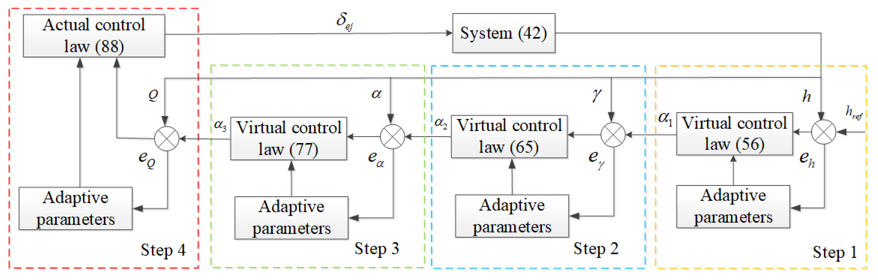
It should be mentioned that backstepping technique is used to construct an adaptive controller for nonlinear system, the recursive design procedure contains four steps. To facilitate the readers’ comprehension, the general block diagram of the proposed control scheme is given in Figure 1.
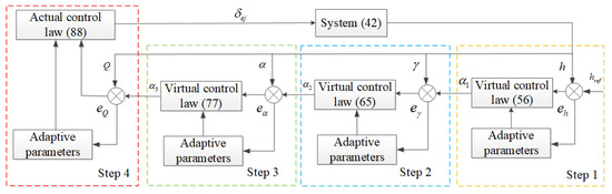
Figure 1.
Block diagram of the height subsystem.
The design of adaptive control law is firstly based on the definition of tracking error
A reduced order function , is introduced before performing the backstepping process design
and a switching function
where a is constant that the designer can design in advance.
According to (21) and (22), the following conclusion can be obtained
and
where n is positive integer.
Next, the detailed controller design process based on backstepping technology is as follows.
3.3.1. Step 1
Firstly, the intermediate control is designed to make the corresponding subsystem (track angle ) toward the equilibrium position.
Consider the altitude subsystem and note the tracking error of altitude h
Choose an improved quadratic Lyapunov function
By introducing , the time derivative of is described as
Define an unknown nonlinear function
Using the general form of neural network (13) to approximate the unknown function , then
where , .
Define
where is a positive design constant.
A new switching regulation function is proposed
Design a virtual controller as follows
where is the estimate of , , , and are positive design constants.
3.3.2. Step 2
Secondly, the intermediate control is designed to make the corresponding subsystem (attack angle ) tend towards equilibrium position.
Consider the tracking error and of track angle
Choose an improved quadratic Lyapunov function
Define an unknown nonlinear function
Using the general form of neural network (13) to approximate unknown functions , to obtain
Similarly, a switching adjustment function is proposed as
Design a virtual controller as follows
where and are positive design constants.
It is worth mentioning that the result of can be obtained through analysis. If , there is obviously , so ; if , then , using Young’s inequality, we obtain
According to the definition in (64) to obtain
3.3.3. Step 3
Thirdly, the intermediate control is designed to make the corresponding (pitch angular velocity Q) subsystem tend towards equilibrium position.
Consider the tracking error of the angle of attack
Choose an improved quadratic Lyapunov function
Define an unknown nonlinear function
Similarly, a switching adjustment function is proposed as
Design a virtual controller as follows
where and are positive design constants.
Similar to Step 2
3.3.4. Step 4
Fourthly, the stabilization of system can be achieved with the actual control input u (elevator deflection angle ) being designed.
Consider the tracking error of the pitch angular velocity Q
Choose an improved quadratic Lyapunov function
Define an unknown nonlinear function
And define
where the unknown parameters and will be estimated by designing an adaptive law.
Next, an auxiliary control law is constructed as follows
where and are positive design constants, is the estimate of and .
Similarly, the switching adjustment function is constructed as follows
Next, construct the actual smoothing control input as
where is a positive design constant.
Design the following adaptive update laws are as
where is the estimation of with estimation error , is a known compact set satisfying .
So far, the design process of the adaptive tracking controller for the height subsystem in the infinite time domain has been completed.
4. Stability Analysis
4.1. Stability Analysis of Speed Subsystem
Theorem 1.
Considering the nonlinear system (18) under Assumption 1, the actual control input (103) is designed by introducing the auxiliary control law (102) and the parameter adaptive update law (104)–(106). The control scheme can ensure that: (1) All the signals of the speed subsystem are bounded; (2) The tracking error can converge to the interval defined by the designer within the prescribe fixed time , i.e., , in which the parameters and can be designed in advance; (3) The speed will not exceed the set of constraints.
Proof.
In order to analyze the stability of the velocity subsystem, the following Lyapunov function is considered
where , , . □
We know the property of the inner projection operator of compact set , so we obtain
Recalling (37) and Lemma 2 to obtain
With inequality , it holds that
According to the result of (97), it is obtained that has the property of non-increasing, so the boundedness of , , and is guaranteed. Since , and are bounded constants, . Because and its derivatives are bounded, . Through similar analysis, all closed-loop signals are bounded.
It is now proven that the proposed control method can allow the tracking error to converge to a range that can be defined by the designer within a predetermined time.
With the help of (97), the following inequality holds
Integrate both sides of (98) to obtain
where indicates .
By applying the Barbalat lemma yields
Therefore, the tracking error asymptotically approaches a prescribe interval in the infinite domain time .
In turn, the adaptive controller in the original nonlinear velocity subsystem (18) is designed. According to the inverse transformation of time scale, in the control law in Section 3.2 is replaced by t, so the prescribe time control is realized through the mapping function from the perspective of time scale.
The auxiliary control law and the actual control input are designed as follows:
The adaptive updating law of parameters is
Similar to the above proof process, consider the following Lyapunov function
where , , .
Along the same lines, we can draw a conclusion
Because the time scale coordinate mapping method is adopted, the prescribe time of the finite field is mapped to the time of the infinite field, which is obtained from (98)–(100)
Therefore, the actual speed tracking error can converge to the interval defined by the designer within the prescribe time . Next, it is proved that the speed will not exceed the set of constraints. Because , and can be designed in advance, if is defined, it can be inferred that there is for , so the conclusion is proved.
So far, the proof of Theorem 1 has been completed.
4.2. Stability Analysis of Altitude Subsystem
Theorem 2.
Considering the nonlinear system (41) under Assumption 2, the actual control input (122) is designed by introducing the auxiliary control law (121) and the parameter adaptive update law(123)–(126). The control scheme can ensure that: (1) all signals of the altitude subsystem are bounded; (2) The tracking error can converge to the interval defined by the designer within the prescribe fixed time , that is, , , in which the parameters and can be designed in advance; (3) All state quantities do not exceed the set of constraints.
Proof.
In order to analyze the stability of the velocity subsystem, the following Lyapunov function is considered
where , , . □
We know the property and of the inner projection operator of compact set , so we obtain
According to (112), is obtained. Therefore, can be further expressed as
According to (88) and Lemma 2, we can obtain
With the inequality yields
According to the result of (116), it is obtained that has the property of non-increasing, so the boundedness of , , and is guaranteed. Since , and are bounded constants, . Because and its derivatives are bounded, . Since is a function of bounded signals, there is , so . Through similar analysis, the boundedness of and Q can be deduced in turn, so all closed-loop signals are bounded.
It is now proven that the proposed control method can allow the height tracking error to converge to a range that can be defined by the designer within a predetermined time.
With the help of (116), the following inequality holds
Take and integrate both sides of (117) to obtain
which indicates that .
Applying the Barbalat lemma yields
Therefore, the tracking error asymptotically approaches a prescribe interval within the time of the infinite domain.
In turn, the adaptive controller in the original nonlinear height subsystem (41) is designed. According to the inverse transformation of time scale, in the control law in Section 3.3 is replaced by t, so the prescribe time control is realized through the mapping function from the perspective of time scale. Similarly, the auxiliary control law and the actual control input are designed as follows:
where the parameter adaptive updating law is
Similarly to the former proof process, consider the following Lyapunov function
where , , .
Along the same lines, we can draw a conclusion
Due to the use of the time scale coordinate mapping method, the prescribe time of the finite field is mapped to the time of the infinite field, as obtained from Equations (117)–(119)
Therefore, the actual height error can converge to the interval defined by the designer within a prescribe time .
Next, it is proven that all state variables will not exceed the set of constraints .
Since and can be designed in advance, if is defined, it can be inferred that . Due to the boundedness of the Lyapunov function , can be obtained. Based on the conclusion of , there must be a normal number such that , and if is defined, there is . Using the similar approach, predefining the value of by the designer, the conclusion of , can be fully guaranteed, that is, none of the state variables will exceed the set of constraints.
At this point, the proof of Theorem 2 was completed.
5. Simulation Results and Analysis
In this section, the simulation results of hypersonic vehicle are given to verify the effectiveness of the proposed controller.
For the longitudinal dynamic model, the initial state is set as velocity ft/s, altitude = 88,000 ft, initial velocity error ft/s, altitude error ft/s, track angle rad, angle of attack rad, pitch angular velocity rad/s, and elastic state quantities , and . The reference trajectories and are generated by a second-order filter , where ft/s and ft. The parameters of the controller are set to , , , ; , , .
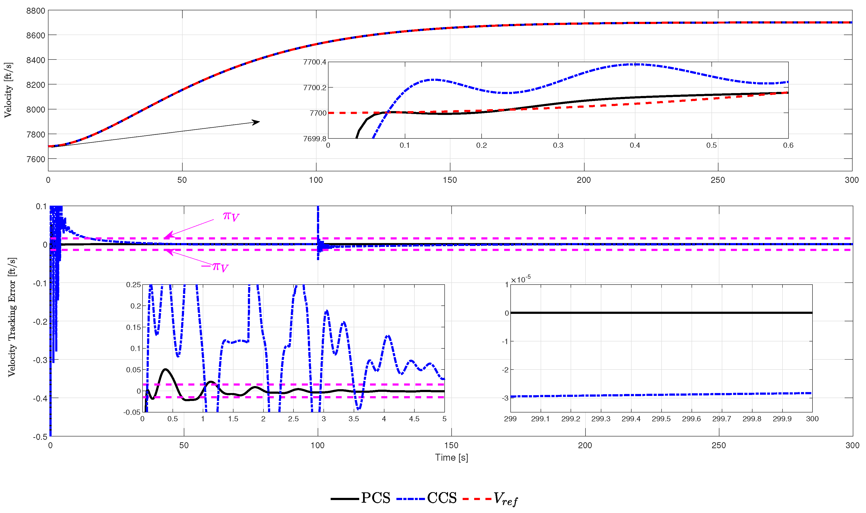
The set scene requires that the tracking error converge to the prescribe range at the prescribe time s, and the height tracking error converge to the prescribe range at the prescribe time s. The analog actuator starts to fail in the 100th second, and the failure parameter is set to , , rad. In order to prove the superiority of the proposed method, it is compared with the traditional control scheme, where PCs represents the proposed control scheme and CCS represents the traditional control scheme.
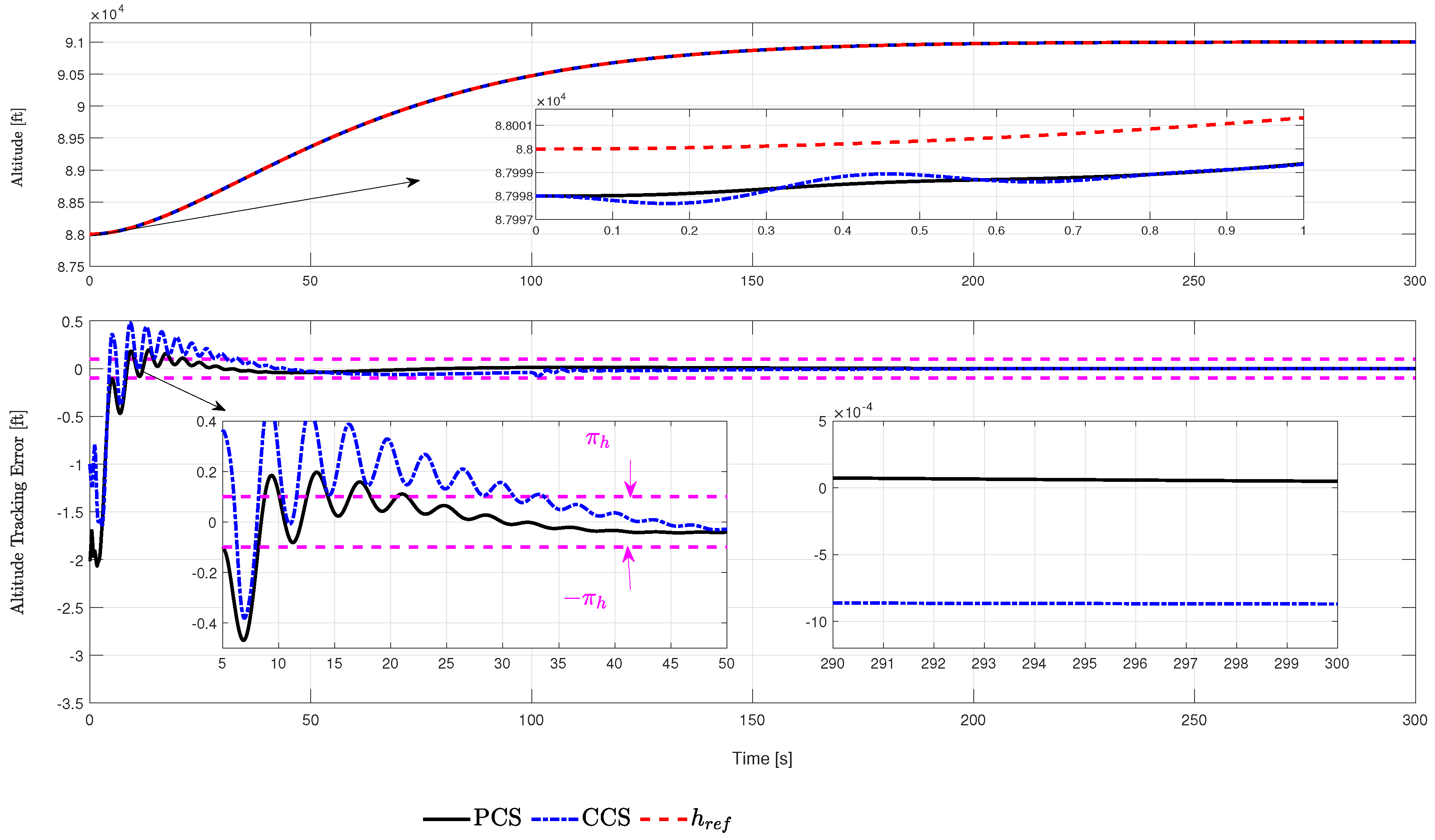
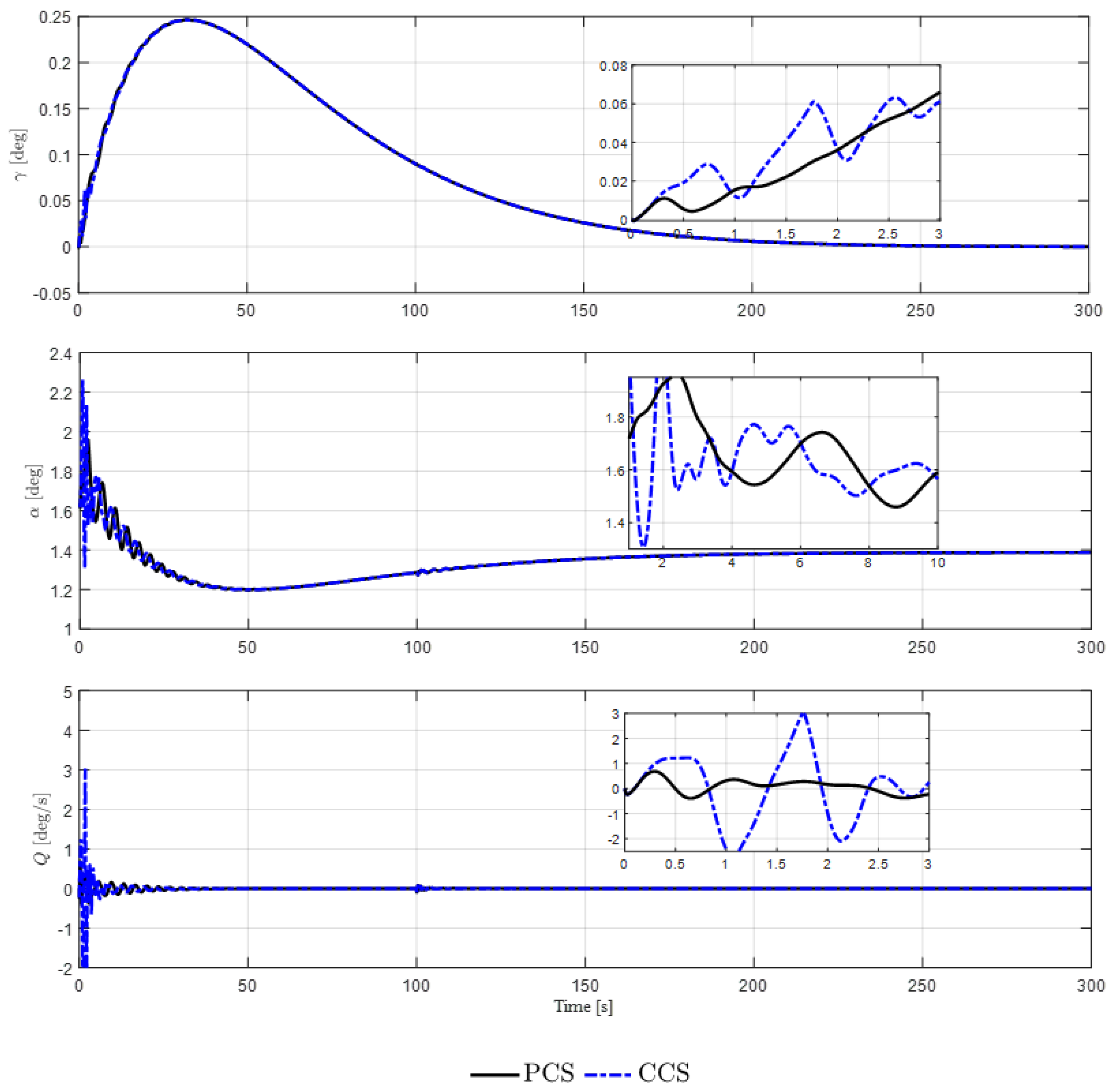
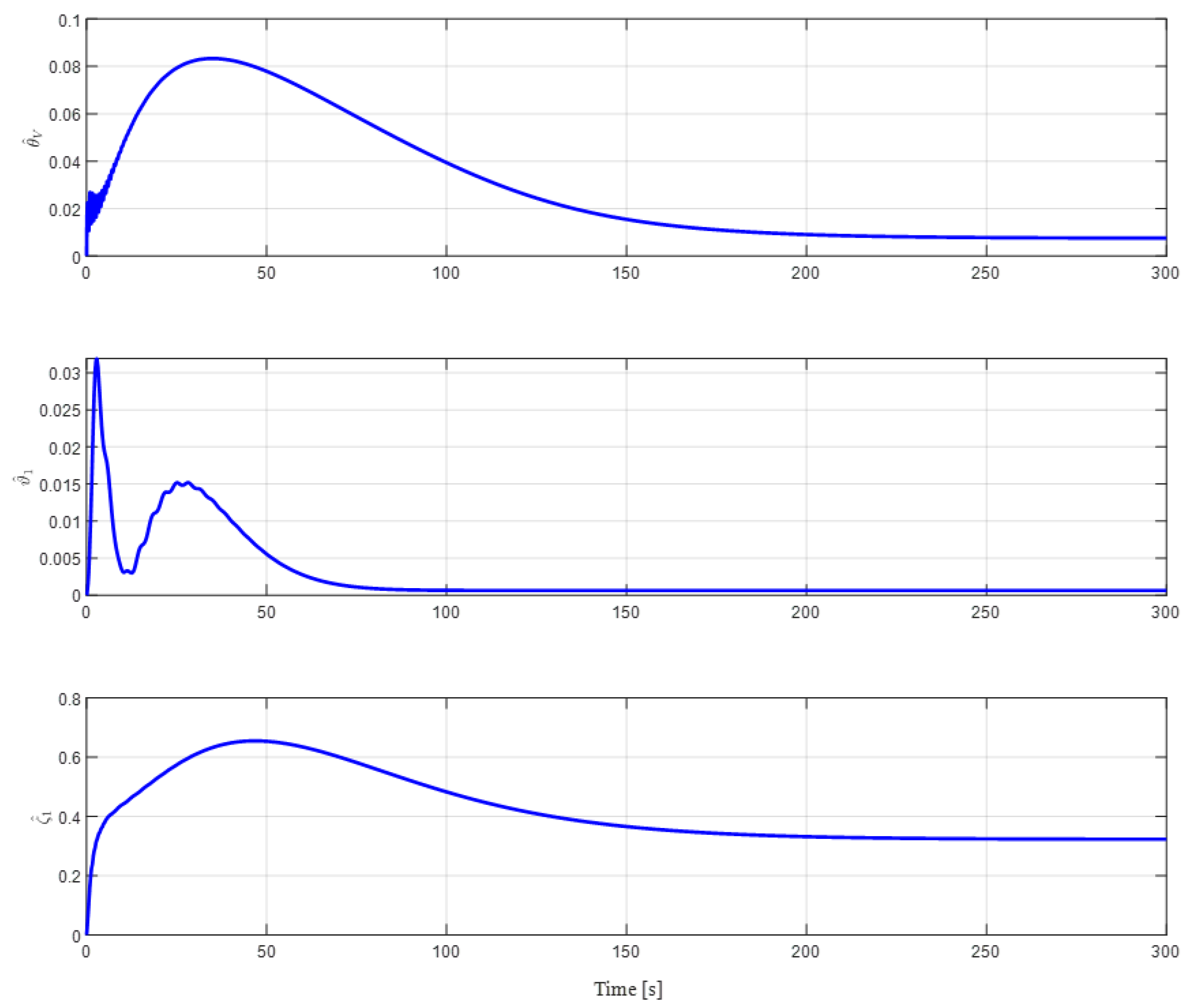
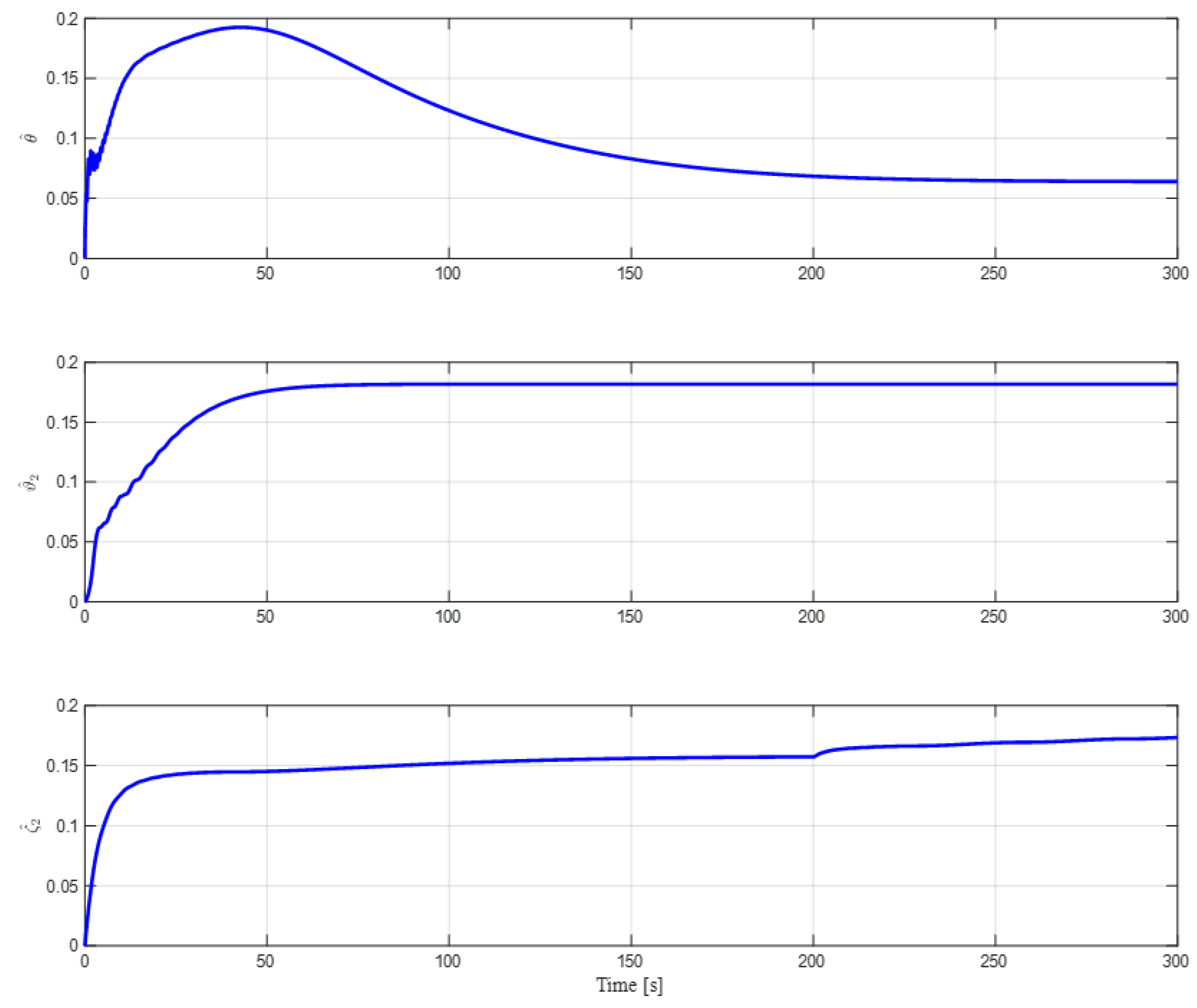
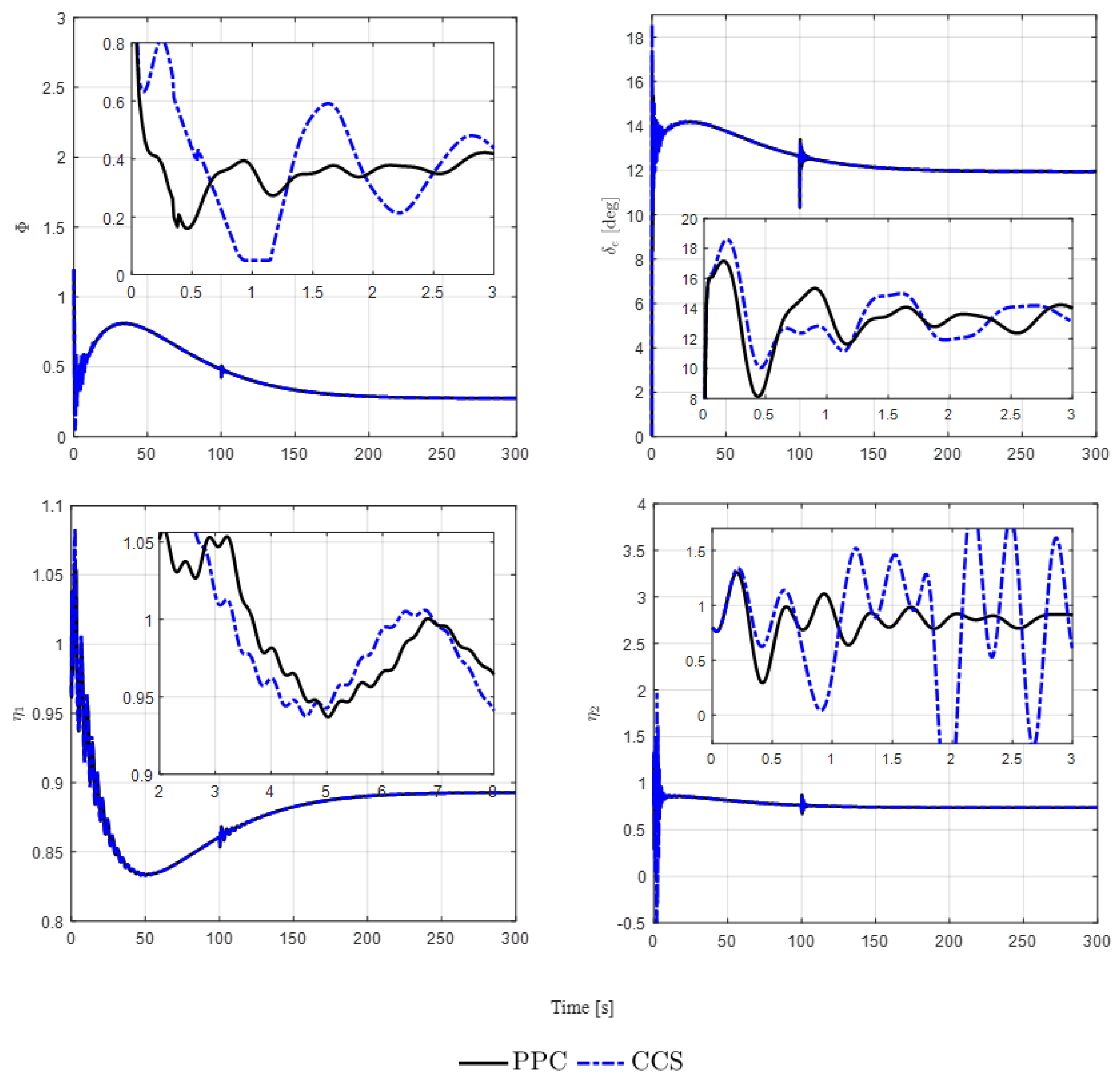
The simulation results are shown in Figure 2, Figure 3, Figure 4, Figure 5, Figure 6 and Figure 7. From Figure 2 and Figure 3, it can be seen that, even considering the actuator fault, the speed and height tracking errors converge to the prescribe range within the prescribe time. In addition to the prescribe time tracking performance, it can also be verified from Figure 2 and Figure 3 that, even if an unknown actuator fault occurs, the speed and height have strong robustness to the tracking of its instructions, will not change greatly and the tracking error can quickly converge to the range prescribed by the designer. Figure 4 shows the three rigid body state quantities , , and Q of HSV. The simulation results show that the state signals are bounded. Figure 5 and Figure 6, respectively, depict the corresponding curves of the adaptive parameters of the HSV speed subsystem and height subsystem. It can be seen that , , , , and are bounded in the process of system control. Figure 7 describes the control input signals and of the designed HSV and the flexible state variables and , it can be concluded that the signals are bounded.
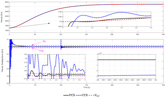
Figure 2.
Speed tracking results with the actuator fault of HSV.
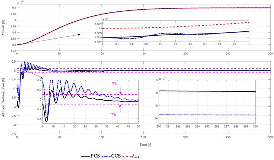
Figure 3.
Height tracking results with the actuator fault of HSV.
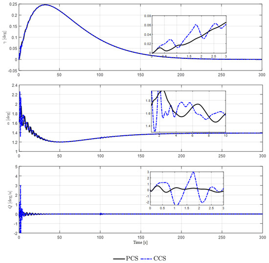
Figure 4.
Response curve of HSV in rigid state , , and Q.
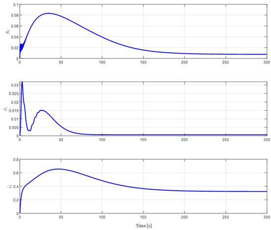
Figure 5.
Adaptive parameters , , and of HSV speed subsystem.
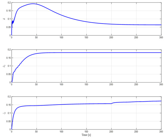
Figure 6.
Adaptive parameters , , and of HSV height subsystem.
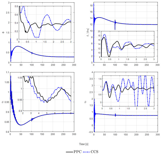
Figure 7.
Actual fuel equivalent ratio , elevator deflection angle , and flexibility state quantity of HSV.
6. Discussion
Compared with the traditional control scheme, the proposed control scheme can meet the different tracking performance requirements, has faster convergence speed and higher convergence accuracy, and better solves the adaptive prescribe time tracking problem with actuator failure. In addition, it is noted that there is no constraint on the tracking error at the beginning of the system performance. This means that, compared with the existing error constraint implementation schemes, the proposed control algorithm does not need to know the initial tracking conditions in advance, and can also achieve the prescribe time tracking performance. Additionally, the selection of actuator fault parameters is based on an appropriate value. If the fault parameters are too large, greater control energy is required and even system stability cannot be ensured. If the fault parameters are too small, the impact of the fault can be ignored, which cannot reflect the progressiveness of the proposed method. Due to the design of two adaptive parameters to estimate unknown faults, the parameters can be adjusted online to achieve adaptive fault-tolerant control when faults occur, thereby enhancing the robustness of the actual flight control system. According to the tracking curve of the speed subsystem, it can be seen that the analog actuator starts to fail in the 100th second. At this time, traditional control methods cannot guarantee that the tracking error converges to the prescribed range of 0.02, and the maximum tracking error even exceeds 0.25 with a chattering phenomenon that occurs. However, the control method proposed in the article can ensure that the tracking error is within the required range.
7. Conclusions
In this paper, the adaptive fault-tolerant tracking control of hypersonic vehicle with prescribe time and tracking error is studied. Firstly, a time scale coordinate mapping function is introduced and the controller is designed in the transformed infinite time domain. An improved Lyapunov function and an improved tuning function are constructed. When the initial tracking conditions are completely unknown, the tracking error converges in the range that can be defined by the designer combined with the Barbalat lemma. At the same time, the online parameter estimation is designed to ensure the adaptive fault-tolerant control of the system. On this basis, it is ensured that the actual tracking errors of speed, altitude, track angle, angle of attack, and pitch rate can converge to the range that can be defined in advance by the designer within the prescribe time. Simulation results verify the effectiveness of the method. The control scheme effectively solves the limitation of the unknown prior knowledge of the initial error, and meets the specific needs of the actual scene. In future research directions, as the system is based on a universal prescribe time architecture, this control strategy is also applicable to other vehicle models, including wing flying aircraft. In addition, this paper focuses on the control of a single aircraft, further research will expand it to the formation control of multiple aircraft.
Author Contributions
Methodology, F.G.; Conceptualization and funding acquisition, W.Z.; data analysis, M.L.; writing, R.Z. All authors have read and agreed to the published version of the manuscript.
Funding
This work was supported by China Postdoctoral Science Foundation (Grant no. 2023M744292).
Data Availability Statement
The data are available from the corresponding author on reasonable request.
Acknowledgments
The authors would like to greatly appreciate the support of National Key Laboratory of Unmanned Aerial Vehicle Technology and The Youth Innovation Team of Shaanxi University. Besides, thanks for the editor and all anonymous reviewers for their comments, which help to improve the quality of this article.
Conflicts of Interest
The authors declare no conflict of interest.
References
- Sun, J.; Pu, Z.; Chang, Y.; Ding, S.; Yi, J. Appointed-Time Control for Flexible Hypersonic Vehicles with Conditional Disturbance Negation. IEEE Trans. Aerosp. Electron. Syst. 2023, 59, 6327–6345. [Google Scholar] [CrossRef]
- Wang, L.; Qi, R.; Wen, L.; Jiang, B. Adaptive Multiple-Model-Based Fault-Tolerant Control for Non-minimum Phase Hypersonic Vehicles with Input Saturations and Error Constraints. IEEE Trans. Aerosp. Electron. Syst. 2023, 59, 519–540. [Google Scholar] [CrossRef]
- Li, B.-Q.; Du, M.-Z.; Zhang, L.-H.; Zong, M.-Z. A comprehensive RFD-FTC-DCA system for hypersonic vehicles with saturation constraints. Int. J. Control 2024, 97, 871–883. [Google Scholar] [CrossRef]
- Lv, M.; De Schutter, B.; Baldi, S. Nonrecursive Control for Formation-Containment of HFV Swarms with Dynamic Event-Triggered Communication. IEEE Trans. Ind. Inform. 2023, 19, 3188–3197. [Google Scholar] [CrossRef]
- Guo, J.; Wang, J.; Guo, Z.; Su, Y. Attitude optimization control of hypersonic flight vehicle considering partially unknown control direction. Trans. Inst. Meas. Control 2023, 45, 1337–1350. [Google Scholar] [CrossRef]
- Lv, M.; De Schutter, B.; Wang, Y.; Shen, D. Fuzzy Adaptive Zero-Error-Constrained Tracking Control for HFVs in the Presence of Multiple Unknown Control Directions. IEEE Trans. Cybern. 2023, 53, 2779–2790. [Google Scholar] [CrossRef] [PubMed]
- Mu, C.; Ni, Z.; Sun, C.; He, H. Air-Breathing Hypersonic Vehicle Tracking Control Based on Adaptive Dynamic Programming. IEEE Trans. Neural Netw. Learn. Syst. 2017, 28, 584–598. [Google Scholar] [CrossRef] [PubMed]
- Basin, M.V.; Yu, P.; Shtessel, Y.B. Hypersonic Missile Adaptive Sliding Mode Control Using Finite- and Fixed-Time Observers. IEEE Trans. Ind. Electron. 2018, 65, 930–941. [Google Scholar] [CrossRef]
- Zhang, Y.; Shou, Y.; Zhang, P.; Han, W. Sliding mode based fault-tolerant control of hypersonic reentry vehicle using composite learning. Neurocomputing 2022, 484, 142–148. [Google Scholar] [CrossRef]
- Hu, X.; Guo, C.; Hu, C.; He, B. Sliding mode learning control for T-S fuzzy system and an application to hypersonic flight vehicle. Asian J. Control 2023, 25, 407–417. [Google Scholar] [CrossRef]
- Zhao, D.; Jiang, B.; Yang, H. Backstepping-Based Decentralized Fault-Tolerant Control of Hypersonic Vehicles in PDE-ODE Form. IEEE Trans. Autom. Control 2022, 67, 1210–1225. [Google Scholar] [CrossRef]
- Bu, X.; Wu, X.; Zhang, R.; Ma, Z.; Huang, J. Tracking differentiator design for the robust backstepping control of a flexible air-breathing hypersonic vehicle. J. Frankl. Inst.-Eng. Appl. Math. 2015, 352, 1739–1765. [Google Scholar] [CrossRef]
- Yu, X.; Li, P.; Zhang, Y. The Design of Fixed-Time Observer and Finite-Time Fault-Tolerant Control for Hypersonic Gliding Vehicles. IEEE Trans. Ind. Electron. 2018, 65, 4135–4144. [Google Scholar] [CrossRef]
- Chao, D.; Qi, R.; Jiang, B. Adaptive fault-tolerant attitude control for hypersonic reentry vehicle subject to complex uncertainties. J. Frankl. Inst.-Eng. Appl. Math. 2022, 359, 5458–5487. [Google Scholar] [CrossRef]
- Han, T.; Hu, Q.; Shin, H.-S.; Tsourdos, A.; Xin, M. Incremental Twisting Fault Tolerant Control for Hypersonic Vehicles with Partial Model Knowledge. IEEE Trans. Ind. Inform. 2022, 18, 1050–1060. [Google Scholar] [CrossRef]
- Wang, L.; Qi, R.; Jiang, B. Adaptive actuator fault-tolerant control for non-minimum phase air-breathing hypersonic vehicle model. ISA Trans. 2022, 126, 47–64. [Google Scholar] [CrossRef] [PubMed]
- Dai, P.; Feng, D.; Feng, W.; Cui, J.; Zhang, L. Entry trajectory optimization for hypersonic vehicles based on convex programming and neural network. Aerosp. Sci. Technol. 2023, 137, 108259. [Google Scholar] [CrossRef]
- Xu, B.; Yang, C.; Pan, Y. Global Neural Dynamic Surface Tracking Control of Strict-Feedback Systems with Application to Hypersonic Flight Vehicle. IEEE Trans. Neural Netw. Learn. Syst. 2015, 26, 2563–2575. [Google Scholar] [CrossRef]
- Bu, X.W.; Xiao, Y.; Lei, H.M. An Adaptive Critic Design-Based Fuzzy Neural Controller for Hypersonic Vehicles: Predefined Behavioral Nonaffine Control. IEEE-ASME Trans. Mechatron. 2019, 24, 1871–1881. [Google Scholar] [CrossRef]
- Wang, P.F.; Wang, J.; Bu, X.W.; Jia, Y.J. Adaptive fuzzy tracking control for a constrained flexible air-breathing hypersonic vehicle based on actuator compensation. Int. J. Adv. Robot. Syst. 2016, 13, 1–11. [Google Scholar] [CrossRef]
- Hu, X.X.; Xu, B.; Hu, C.H. Robust Adaptive Fuzzy Control for HFV with Parameter Uncertainty and Unmodeled Dynamics. IEEE Trans. Ind. Electron. 2018, 65, 8851–8860. [Google Scholar] [CrossRef]
- Chen, H.; Wang, P.; Tang, G. Fuzzy Disturbance Observer-Based Fixed-Time Sliding Mode Control for Hypersonic Morphing Vehicles with Uncertainties. IEEE Trans. Aerosp. Electron. Syst. 2023, 59, 3521–3530. [Google Scholar] [CrossRef]
- Bu, X.; Qi, Q. Fuzzy Optimal Tracking Control of Hypersonic Flight Vehicles via Single-Network Adaptive Critic Design. IEEE Trans. Fuzzy Syst. 2022, 30, 270–278. [Google Scholar] [CrossRef]
- Zhang, H.; Wang, P.; Tang, G.; Bao, W. Fuzzy disturbance observer-based dynamic sliding mode control for hypersonic morphing vehicles. Aerosp. Sci. Technol. 2023, 142, 108633. [Google Scholar] [CrossRef]
- Xu, B.; Wang, D.; Zhang, Y.; Shi, Z. DOB-Based Neural Control of Flexible Hypersonic Flight Vehicle Considering Wind Effects. IEEE Trans. Ind. Electron. 2017, 64, 8676–8685. [Google Scholar] [CrossRef]
- Dong, M.; Xu, X.; Xie, F. Constrained Integrated Guidance and Control Scheme for Strap-Down Hypersonic Flight Vehicles with Partial Measurement and Unmatched Uncertainties. Aerospace 2022, 9, 840. [Google Scholar] [CrossRef]
- Ding, Y.; Yue, X.; Liu, C.; Dai, H.; Chen, G. Finite-time controller design with adaptive fixed-time anti-saturation compensator for hypersonic vehicle. ISA Trans. 2022, 122, 96–113. [Google Scholar] [CrossRef] [PubMed]
- Guo, Y.; Xu, B. Finite-Time Deterministic Learning Command Filtered Control for Hypersonic Flight Vehicle. IEEE Trans. Aerosp. Electron. Syst. 2022, 58, 4214–4225. [Google Scholar] [CrossRef]
- Yu, X.; Li, P.; Zhang, Y. Fixed-Time Actuator Fault Accommodation Applied to Hypersonic Gliding Vehicles. IEEE Trans. Autom. Sci. Eng. 2021, 18, 1429–1440. [Google Scholar] [CrossRef]
- Lv, M.; Li, Y.; Wan, L.; Dai, J.; Chang, J. Fast Nonsingular Fixed-Time Fuzzy Fault-Tolerant Control for HFVs with Guaranteed Time-Varying Flight State Constraints. IEEE Trans. Fuzzy Syst. 2022, 30, 4555–4567. [Google Scholar] [CrossRef]
- Dong, Z.; Li, Y.; Lv, M. Adaptive nonsingular fixed-time control for hypersonic flight vehicle considering angle of attack constraints. Int. J. Robust Nonlinear Control 2023, 33, 6754–6777. [Google Scholar] [CrossRef]
- Zhang, H.; Wang, P.; Tang, G.; Bao, W. Fixed-time sliding mode control for hypersonic morphing vehicles via event-triggering mechanism. Aerosp. Sci. Technol. 2023, 140, 108458. [Google Scholar] [CrossRef]
- Bolender, M.A.; Doman, D.B. Nonlinear Longitudinal Dynamical Model of an Air-Breathing Hypersonic Vehicle. J. Spacecr. Rocket. 2007, 44, 374–387. [Google Scholar] [CrossRef]
- Zhang, W.; Dong, W.; Lv, M.; Liu, Z.; Zhou, Y.; Feng, H. Barrier Lypunov functions-based nonsingular fixed-time switching control for strict-feedback nonlinear dynamics with full state constraints. Int. J. Robust Nonlinear Control 2021, 31, 7862–7885. [Google Scholar] [CrossRef]
Disclaimer/Publisher’s Note: The statements, opinions and data contained in all publications are solely those of the individual author(s) and contributor(s) and not of MDPI and/or the editor(s). MDPI and/or the editor(s) disclaim responsibility for any injury to people or property resulting from any ideas, methods, instructions or products referred to in the content. |
© 2024 by the authors. Licensee MDPI, Basel, Switzerland. This article is an open access article distributed under the terms and conditions of the Creative Commons Attribution (CC BY) license (https://creativecommons.org/licenses/by/4.0/).