Multiple Unmanned Aerial Vehicle (multi-UAV) Reconnaissance and Search with Limited Communication Range Using Semantic Episodic Memory in Reinforcement Learning

Abstract

Unmanned Aerial Vehicles (UAVs) have garnered widespread attention in reconnaissance and search operations due to their low cost and high flexibility. However, when multiple UAVs (multi-UAV) collaborate on these tasks, a limited communication range can restrict their efficiency. This paper investigates the problem of multi-UAV collaborative reconnaissance and search for static targets with a limited communication range (MCRS-LCR). To address communication limitations, we designed a communication and information fusion model based on belief maps and modeled MCRS-LCR as a multi-objective optimization problem. We further reformulated this problem as a decentralized partially observable Markov decision process (Dec-POMDP). We introduced episodic memory into the reinforcement learning framework, proposing the CNN-Semantic Episodic Memory Utilization (CNN-SEMU) algorithm. Specifically, CNN-SEMU uses an encoder–decoder structure with a CNN to learn state embedding patterns influenced by the highest returns. It extracts semantic features from the high-dimensional map state space to construct a smoother memory embedding space, ultimately enhancing reinforcement learning performance by recalling the highest returns of historical states. Extensive simulation experiments demonstrate that in reconnaissance and search tasks of various scales, CNN-SEMU surpasses state-of-the-art multi-agent reinforcement learning methods in episodic rewards, search efficiency, and collision frequency.

1. Introduction

Advancements in flight control systems, endurance capabilities, and sensors have significantly expanded the use of Unmanned Aerial Vehicles (UAVs) in fields such as search and rescue (SAR) [1], military reconnaissance [2], and environmental monitoring [3]. Compared to traditional human-crewed aircraft or satellite reconnaissance methods, coordinating multiple UAVs (multi-UAV) for reconnaissance and search operations offers lower operational costs and greater flexibility. Additionally, UAVs can be equipped with various sensors to perform diverse reconnaissance and search tasks. Therefore, studying multi-UAV collaborative reconnaissance and search (MCRS) is highly important.

However, coordinating multi-UAVs for reconnaissance and search presents numerous challenges. First, effective communication between UAVs is necessary for information fusion. Thus, it is crucial to consider multi-UAV cooperative reconnaissance and search with a limited communication range (MCRS-LCR). Second, precise planning of each UAV’s flight path is required to ensure comprehensive search area coverage while avoiding collisions and path overlaps. Finally, UAVs need to make distributed decisions based on environmental changes and mission requirements, maintaining system robustness in case of a single-point failure. Additionally, target locations are often unknown and may be sparsely distributed over a vast, unexplored area [4]. If reconnaissance sensors have errors and UAVs fail to detect targets on the first attempt, revisiting the area becomes challenging. These factors all contribute to the complexity of the MCRS-LCR problem.

To address the MCRS-LCR problem, current research primarily focuses on UAV cooperative control and search strategies. Cooperative control can be divided into centralized and distributed structures. Distributed control allows UAVs to make autonomous decisions without a command center, enhancing system scalability and resistance to interference. This has become the leading research direction in UAV control [5]. Regardless of the control structure, communication between UAVs is crucial for effective coordination. Oliehoek [6] categorizes communication among multiple agents into explicit, implicit, delayed, costly, and local communication. Based on these classifications, many researchers consider communication factors when exploring UAV target search problems [7,8,9]. However, for the MCRS-LCR problem, questions like “when to communicate” and “what to communicate” still require further investigation.

Regarding reconnaissance search strategies, some studies discretize the reconnaissance space and generate target probability maps to represent the probability distribution of target locations [7,8,10,11,12]. This method accounts for UAV reconnaissance sensor errors and performs well in practical applications. Other studies have developed optimization methods for multi-UAV systems based on heuristic algorithms [13], ant colony algorithms [14], and particle swarm algorithms [15]. However, as the number of UAVs increases and the environmental state space expands, these methods are prone to local optima.

Deep reinforcement learning (DRL) [16] offers powerful learning capabilities, providing new solutions to the MCRS-LCR problem. Multi-agent deep reinforcement learning (MADRL) further extends DRL’s application scope. MADRL commonly employs the Centralized Training with Decentralized Execution (CTDE) framework. During training, agents use global information and share knowledge to enhance collaboration. During execution, each agent chooses actions based on local observations, enabling distributed decision-making. This approach has succeeded significantly in StarCraft II [17], autonomous driving [18], and multi-robot formation [19].

In deep reinforcement learning, agents need to interact with the environment hundreds or thousands of times to reach human-level performance [20], resulting in data inefficiency. Unlike traditional reinforcement learning methods, human learning relies not only on interactions with the environment but also on past experiences stored in the hippocampus [21], a process known as episodic memory. However, recalling detailed episodes is often impossible. Instead, the human brain typically recalls features associated with high rewards. Episodic memory uses these features to guide future behavior (Figure 1). Research suggests that the ventral hippocampus may encode reward-related information and extract abstract features from environmental states [22,23,24], known as memory representation. This suggests that embedding semantic information with rewards into state space encoding can enhance the effectiveness fo episodic memory.

Inspired by hippocampal episodic memory, Blundell et al. [25] proposed introducing episodic memory into reinforcement learning to improve learning efficiency. Zheng et al. [26], Hyungho et al. [27], and Ma [28] have used episodic memory in MADRL. However, the state space dimension in MADRL increases with the number of agents, making extracting semantic features from high-dimensional map state spaces in the MCRS-LCR problem particularly challenging. To efficiently utilize episodic memory by extracting semantic features from high-dimensional map state spaces, we draw an analogy to vision-based state spaces. An encoder–decoder structure with a CNN is used to learn state embedding patterns influenced by the highest returns. We call this method CNN-Semantic Episodic Memory Utilization (CNN-SEMU).

This paper explores the cooperative reconnaissance and search of unknown static targets using multiple UAVs with limited communication range. The main contributions are as follows:

• A communication and information fusion model for the MCRS-LCR problem based on belief maps is proposed. Each UAV maintains a belief map for all UAVs and uses a max-plus-sum approach for information fusion, enabling effective communication.
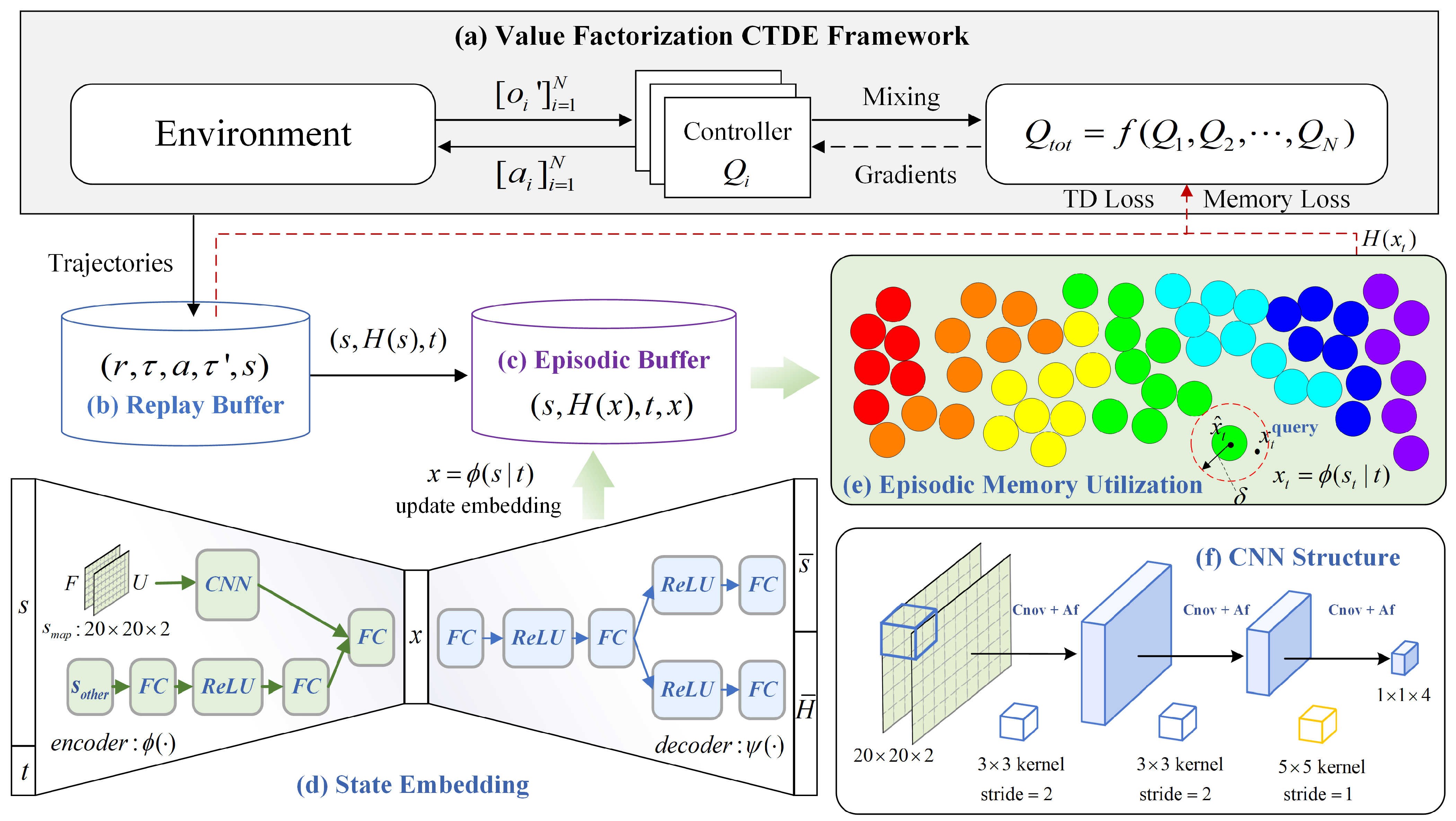
• Episodic memory is introduced into the MCRS-LCR problem. Using the value factorization centralized training with a decentralized execution (CTDE) framework, episodic memory leverages the highest state values stored in memory to generate better Temporal Difference targets, enhancing MADRL performance.
• A new MADRL method called CNN-Semantic Episodic Memory Utilization (CNN-SEMU) is proposed. CNN-SEMU employs an encoder–decoder structure with a CNN to extract semantic features with the highest returns from high-dimensional map state spaces, enhancing the effectiveness of episodic memory.

The rest of the paper is structured as follows: Section 2 introduces related work. Section 3 provides the system description and problem formulation. Section 4 reformulates the MCRS-LCR problem within the reinforcement learning framework. Section 5 introduces episodic memory into multi-UAV reinforcement learning and proposes the CNN-SEMU algorithm. Section 6 presents the experiments. Section 7 concludes the paper.

2. Related Work

This section briefly reviews current research on UAV communication modes, reconnaissance and search strategies, and episodic memory in reinforcement learning. It also identifies the gaps in these studies regarding the MCRS-LCR problem.

2.1. UAV Communication and Search Strategies

Communication between UAVs is crucial for efficient coordination. Explicit and implicit communication models do not consider communication costs, noise, and timing. In explicit communication [6], communication actions are added to the UAV’s action set, allowing UAVs to communicate by executing these actions. In contrast, implicit communication influences other UAVs’ observations through behavior without direct communication actions.

In [9], a communication topology matrix for UAVs is designed, represented as the Nth power of the UAV adjacency communication matrix. Communication between UAVs is achieved by exchanging digital pheromones. This method effectively represents the communication links between UAVs, but the matrix power calculation is computationally expensive. In [8], UAVs communicate by broadcasting the positive and negative detection times to their neighbors, taking the maximum value within the communication range. Although this method reduces communication volume, it does not accurately reflect the cumulative detection counts by neighboring UAVs. In [7], it is assumed that all UAVs are directly interconnected, simplifying calculations, but it may lead to network congestion with many UAVs communicating simultaneously. If UAV reconnaissance and search are likened to marking a chalkboard, implicit communication can be represented as other UAVs within the communication range instantly observing the mark. In this paper, we continue to study multi-UAV information fusion based on implicit communication.

The target probability map provides UAVs with probabilistic information about target distribution, which they use to optimize reconnaissance and search strategies. The studies [8,10,12] treat the existence of a target in each cell as a $0-1$ distributed random variable. The target probability map can be updated using Bayes’ rule given an initial prior probability. However, if the prior probability is unavailable or incorrect, this method may affect the posterior probability calculation. The studies [7,11] use sensor readings as evidence sources and update the target probability map using Dempster–Shafer (DS) evidence theory. This method does not depend on prior probabilities and can effectively handle conflicting evidence when sensor readings are erroneous.

2.2. Episodic Memory in Reinforcement Learning

In single-agent reinforcement learning, Model-Free Episodic Control (MFEC) [25] uses episodic memory to solve sequential decision tasks. It stores the highest returns of explored state–action pairs in a tabular memory and greedily selects actions based on the maximum returns in the table. Since identical states are challenging to reproduce in natural environments, MFEC generalizes and embeds similar states using k-nearest neighbors and random projection techniques. Episodic Memory Deep Q-Networks (EMDQN) [29] use episodic memory to supervise agent training, combining the generalization strength of Deep Q-Networks (DQN) with the fast convergence of Episodic Control (EC), enabling quicker learning of better policies.

In multi-agent reinforcement learning, the state space dimension is usually more extensive, requiring adjustments and extensions to the feature embedding structures and learning frameworks from single-agent reinforcement learning. Zheng et al. [26] proposed Episodic Multi-agent Reinforcement Learning with Curiosity-driven Exploration (EMC), which introduces episodic memory into cooperative MADRL. EMC uses episodic memory to remember high-return states and employs one-step Temporal Difference (TD) memory targets for regularized learning. However, EMC still uses random projection for state embedding. According to the Johnson–Lindenstrauss lemma [30], random projection can approximately preserve the distance relationships of the original space. However, when the original state changes slightly, the embedded space may fluctuate significantly. Hyungho et al. [27] proposed Efficient Episodic Memory Utilization (EMU), which uses an encoder–decoder structure to learn semantic state embeddings, addressing the sparse selection of semantically similar memories caused by random projection. However, extracting semantic features directly from high-dimensional map state spaces is challenging. Additionally, EMU employs episodic incentives, providing extra rewards for states within desirable trajectories, thereby encouraging desirable state transitions. Desirable trajectories are defined as those that achieve the overall goal or exceed a preset reward threshold. However, the overall goal may be challenging in practical tasks, and the preset reward threshold requires additional domain knowledge. For the MCRS-LCR problem, if targets are sparsely distributed over a large area, it will be challenging to discover all targets, making additional episodic incentives less effective. In this paper, we continue to use regularized memory targets to improve one-step TD learning and employ an encoder–decoder structure with a CNN to learn state embedding patterns influenced by the highest returns.

3. System Description and Problem Formulation

This section describes the system model, including the grid reconnaissance environment, the UAV model, the belief probability map model, and the UAV communication and information fusion model. Building on this, the MCRS-LCR is framed as a multi-objective optimization problem.

Table 1. Main notations in Section 3.

Notation	Description
$c_{x,y}$	Cell at row x and column y in the map.
$u_{i,t}$	The position of UAV i at time step t.
$z_k$	The position of the no-fly zone k.
N	Number of UAVs.
$N_Z$	Number of no-fly zones.
$f_{x,y}^i\left(t\right)$	Sensor data from UAV i at time step t for $c_{x,y}$.
$m_{x,y}^t\left(U\right),m_{x,y}^t\left(F\right),m_{x,y}^t\left(E\right)$	Basic probability assignments for the uncertainty and target maps at time step t for $c_{x,y}$.
$m_b\left(U\right),m_b\left(F\right),m_b\left(E\right)$	Sensors’ basic probability assignments for the uncertainty and target maps.
$N_{x,y}^{i,t}(+),N_{x,y}^{i,t}(-)$	At time step t, the positive and negative detection times of UAV i for $c_{x,y}$.
$m_f,m_e$	The belief that the sensor both identified and failed to identify the target.
$R_c$	The communication range of the UAV.
$N{e}_{i,t}$	Neighbors of UAV i at time step t.
$\tau$	The threshold at which the target is deemed to exist.
$d_1$	No-fly zone safety distances.
$d_2$	Safe distance for UAVs to avoid collisions.

summarizes the main symbols used in this section.

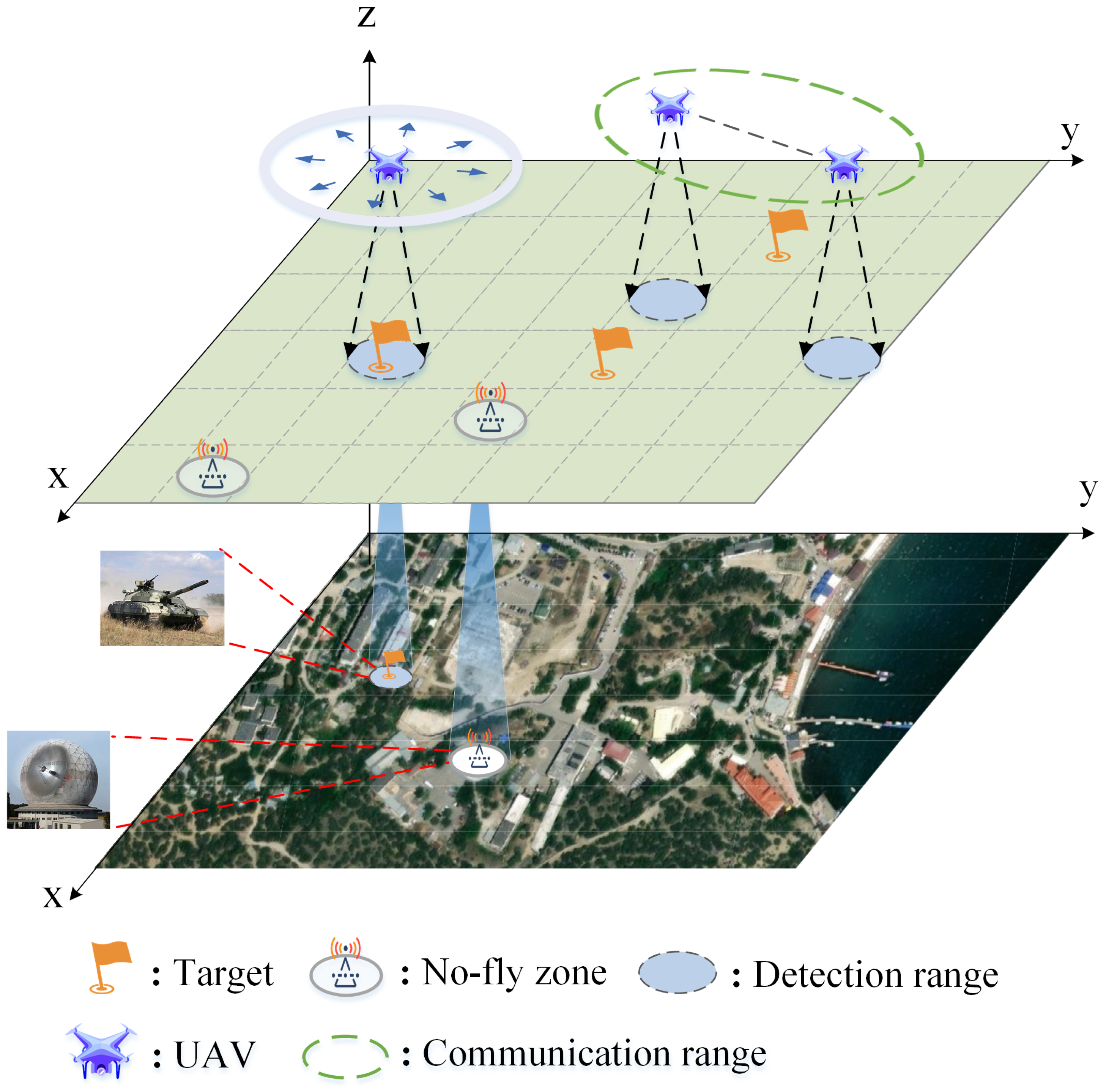
3.1. Reconnaissance Environment Model

As shown in Figure 2, the task area is divided into $L_1\times L_2$ square cells, with the cell in the ith row and jth column denoted as $c_{x,y}$, where $i\in \left\{1,2,\cdots ,L_1\right\}$ and $j\in \left\{1,2,\cdots ,L_2\right\}$. It is assumed that several static targets are distributed within the task area, each occupying one cell, with at most one target per cell. Each cell has two possible states: empty (E), indicating no target is present, or full (F), indicating a target is present. Since there is no prior information about target locations, UAVs must use reconnaissance sensors to search for targets.

Additionally, specific cells in the map are assumed to be inaccessible to UAVs due to no-fly zones or obstacles. UAVs can avoid obstacles using a circular field of view (FOV). Let $z_k$ represent the location of the kth no-fly zone cell, and assume no targets exist within these no-fly zones.

3.2. UAV Model

The distributed UAV system comprises N homogeneous UAVs that collaboratively perform reconnaissance and search tasks. The entire task process is divided into T time steps. At each time step, a UAV searches only the cell at its current position and decides the next step’s search direction, making the action space discrete. The size of each cell depends on the UAV’s reconnaissance performance and the time step setting. For example, if a UAV can complete the reconnaissance of a cell with 100-m sides in 10 min, then the cell size is set to 100 m, and the time step is set to 10 min.

Each UAV has eight possible search directions at each time step. The position of a UAV can be identified by the cell it occupies. Let the position of UAV i at time step t be $u_{i,t}(x,y)$, which is updated by the chosen action a, represented as

$$\left\{\begin{array}{c}{u}_{i,t+1}\left(x\right)=u_{i,t}\left(x\right)+\Delta x\hfill \\ u_{i,t+1}\left(y\right)=u_{i,t}\left(y\right)+\Delta y,\hfill \end{array}\right.$$

(1)

where

$$\Delta (x,y)=\left\{\begin{array}{cc}(-1,0),\hfill & \mathrm{if}a=0\left(\mathrm{left}\right)\hfill \\ (1,0),\hfill & \mathrm{if}a=1\left(\mathrm{right}\right)\hfill \\ (0,-1),\hfill & \mathrm{if}a=2\left(\mathrm{down}\right)\hfill \\ (0,1),\hfill & \mathrm{if}a=3\left(\mathrm{up}\right)\hfill \\ (-1,-1),\hfill & \mathrm{if}a=4(\mathrm{lower}\mathrm{left})\hfill \\ (1,-1),\hfill & \mathrm{if}a=5(\mathrm{lower}\mathrm{right})\hfill \\ (1,1),\hfill & \mathrm{if}a=6(\mathrm{upper}\mathrm{right})\hfill \\ (-1,1),\hfill & \mathrm{if}a=7(\mathrm{upper}\mathrm{left}).\hfill \end{array}\right.$$

(2)

If a UAV’s action would cause it to exceed the task area’s boundaries, that action is removed from the set of possible actions. This discrete action space modeling for UAVs eliminates the need to consider complex dynamics and control issues, such as motion posture and turning radius in continuous space, thereby simplifying the problem and improving path planning efficiency.

Assume all UAVs are equipped with identical reconnaissance sensors and each UAV completes the reconnaissance of its current cell within one step. If UAV i performs reconnaissance in $c_{x,y}$ at time step t, the sensor reading is $f_{x,y}^i\left(t\right)$. If $f_{x,y}^i\left(t\right)=F$, a target is found in $c_{x,y}$; if $f_{x,y}^i\left(t\right)=E$, no target is found. Due to noise and other errors, the sensors may produce false readings, leading to conflicting reconnaissance results. To address this issue, we treat the sensor readings as evidence and use the Dempster–Shafer (DS) evidence theory, as established in [7], to handle these conflicts. By fusing the sensor readings, we can measure the uncertainty of each cell and represent the uncertainty of all cells as a belief probability map.

3.3. Belief Probability Maps

Given that each cell can be in one of two states, E or F, the frame of discernment $\Lambda$ is defined as the power set of these states based on the DS evidence theory:

$$\Lambda =\{E,F,U\},$$

(3)

where $U=\{E,F\}$ represents the uncertain state. A probability can be assigned to each subset in the frame of discernment using the basic probability assignment (BPA) function m. This results in the belief probability map:

$$\sum _{A\in \Lambda }{m}_{x,y}\left(A\right)=\underset{TargetMap}{\underbrace{m_{x,y}\left(E\right)+m_{x,y}\left(F\right)}}+\underset{UncertaintyMap}{\underbrace{m_{x,y}\left(U\right)}}=1,$$

(4)

where the target map $m_{x,y}\left(F\right)$ and $m_{x,y}\left(E\right)$ represent the belief in the presence and absence of a target in $c_{x,y}$, respectively, while the uncertainty map $m_{x,y}\left(U\right)$ represents the uncertainty of $c_{x,y}$. Without prior information, the belief probability map is initialized as $m_{x,y}^{t=0}\left(E\right)=0$, $m_{x,y}^{t=0}\left(F\right)=0$, and $m_{x,y}^{t=0}\left(U\right)=1$.

The core concepts of DS evidence theory are “evidence” and “combination”. “Evidence” refers to sensor readings containing uncertain information, while “combination” refers to the combination rules. According to DS combination rules, sensor readings can be fused as evidence into the belief map at the current time step, thereby updating the belief map for the next time step:

$$\begin{array}{cc}\hfill m_{x,y}^{t+1}(E/F/U)& =m_{x,y}^t\oplus m_b(E/F/U)\hfill \\ \hfill & ={\displaystyle \frac{1}{k}}\sum _{B\cap C=E/F/U}{m}_{x,y}^t\left(B\right)\times m_b\left(C\right),\forall B,C\in \Lambda ,\hfill \end{array}$$

(5)

where

$$k=1-\sum _{B\cap C=\varnothing }{m}_{x,y}^t\left(B\right)\times m_b\left(C\right),\forall B,C\in \Lambda ,$$

(6)

where $m_b$ represents the sensor evidence’s BPA. When a sensor detects a target, this reading can be used as evidence to increase confidence in F. Since no information is provided about the absence of a target, the probability assigned to E is 0. Due to sensor errors, this evidence is not entirely reliable, so the remaining probability is assigned to U. Thus, the evidence for detecting a target is represented as

$$\left\{\begin{array}{c}{m}_b\left(F\right)=m_f\hfill \\ m_b\left(E\right)=0\hfill \\ m_b\left(U\right)=1-m_f.\hfill \end{array}\right.$$

(7)

Likewise, the evidence for the sensor not detecting a target is represented as

$$\left\{\begin{array}{c}{m}_b\left(F\right)=0\hfill \\ m_b\left(E\right)=m_e\hfill \\ m_b\left(U\right)=1-m_e,\hfill \end{array}\right.$$

(8)

where $m_f$ and $m_e$ represent the sensor’s confidence in detecting or not detecting a target, respectively. These values can be obtained from historical statistical data.

3.4. UAV Communication and Information Fusion Model

Each UAV maintains a distributed belief map and cannot access the global map. Therefore, UAVs must enhance their collaboration through information exchange and fusion. While [7] assumes fully connected communication among UAVs, UAVs can only exchange information with their neighbors within the communication range. The neighbors of UAV i are defined as

$$N{e}_{i,t}=\left\{u_{j,t}\right|{∥u_{j,t}-u_{i,t}∥}_2<R_c,j=1,2,\cdots ,N,j\ne i\},$$

(9)

where $R_c$ is the communication range of the UAV. The premise of information fusion is that the belief probability map is independent of the order of detection results. Therefore, we introduce positive and negative detection times. For each cell, a UAV records the positive detection times $N_{x,y}^{i,t}(+)$ and the negative detection times $N_{x,y}^{i,t}(-)$. Their update method is represented as

$$\left\{\begin{array}{cc}{N}_{x,y}^{i,t+1}(+)=N_{x,y}^{i,t}(+)+1\hfill & \mathrm{if}{f}_{x,y}^i\left(t\right)=F\hfill \\ N_{x,y}^{i,t+1}(-)=N_{x,y}^{i,t}(-)+1\hfill & \mathrm{if}{f}_{x,y}^i\left(t\right)=E.\hfill \end{array}\right.$$

(10)

Ref. [7] demonstrated that the state of the belief map depends only on the positive and negative detection times, regardless of the order of detection results. Thus, the recursive formula in Equation (5) can be written to include only the positive and negative detection times. Each UAV can broadcast its positive and negative detection times to its neighbors within the communication range for information fusion, resulting in a distributed belief map for each UAV. It is important to note that our communication model assumes noiseless, instantaneous broadcast communication. This means each UAV broadcasts its messages and immediately receives messages from all other UAVs within its communication range without errors.

Assume each UAV maintains a map of the positive and negative detection times for all UAVs. When UAV j enters the communication range of UAV i, UAV j merges its distributed map with UAV i’s distributed map. After information fusion, the positive and negative detection times for UAV i are represented as

$$N_i=\sum _{q=1}^{N}max(N_{i,q},N_{j,q}),j\ne i.$$

(11)

In the above equation, we denote $N_{x,y}^{i,j,t}(+/-)$ simply as $N_{i,j}$ for conciseness. Equation (11) represents a process of taking the maximum value for each UAV and then summing them. For example, in a multi-UAV system with three UAVs, at time step t, UAV A’s positive detection times for $c_{x,y}$ are $A3B1C0$. This indicates that UAV A’s distributed map records $c_{x,y}$ being detected by UAV A three times, by UAV B once, and by UAV C zero times. When UAV B enters A’s communication range with positive detection times $A1B3C1$ for $c_{x,y}$, the information fusion updates UAV A’s positive detection times to $A3B3C1$, resulting in seven positive detections. In contrast, using the method from [8], which takes the maximum detection times within the communication range, the fused positive detection count would be five, which does not accurately reflect the actual situation.

Denote ${(1-m_f)}^{N_{x,y}^{i,t}(+)}$ as $f_{x,y}^{i,t}$ and ${(1-m_e)}^{N_{x,y}^{i,t}(-)}$ as $e_{x,y}^{i,t}$. Under the initial conditions, the distributed target map and uncertainty map for UAV i after information fusion can be recursively calculated as

$$\left\{\begin{array}{c}{m}_{x,y}^{i,t}\left(E\right)={\displaystyle \frac{f_{x,y}^{i,t}-e_{x,y}^{i,t}\times f_{x,y}^{i,t}}{f_{x,y}^{i,t}+e_{x,y}^{i,t}-e_{x,y}^{i,t}\times f_{x,y}^{i,t}}}\hfill \\ m_{x,y}^{i,t}\left(F\right)={\displaystyle \frac{e_{x,y}^{i,t}-e_{x,y}^{i,t}\times f_{x,y}^{i,t}}{f_{x,y}^{i,t}+e_{x,y}^{i,t}-e_{x,y}^{i,t}\times f_{x,y}^{i,t}}}\hfill \\ m_{x,y}^{i,t}\left(U\right)={\displaystyle \frac{e_{x,y}^{i,t}\times f_{x,y}^{i,t}}{f_{x,y}^{i,t}+e_{x,y}^{i,t}-e_{x,y}^{i,t}\times f_{x,y}^{i,t}}}.\hfill \end{array}\right.$$

(12)

3.5. Problem Formulation

The MCRS-LCR problem requires multi-UAV to reduce uncertainty in the task area and discover as many targets as possible with limited communication. UAVs must avoid no-fly zones and prevent collisions with other UAVs during flight. Therefore, a multi-objective optimization model is established as follows:

Objective function:

$$min\sum _{x=1}^{L_x}\sum _{y=1}^{L_y}{m}_{x,y}^{t=T}\left(U\right),$$

(13)

$$max\sum _{x=1}^{L_x}\sum _{y=1}^{L_y}\mathbb{I}(m_{x,y}^{t=T}\left(F\right)\ge \tau ),$$

(14)

where $\mathbb{I}$ is an indicator function that equals 1 when the condition inside the parentheses is met, and 0 otherwise. $\tau$ represents the threshold for the presence of a target in a cell; when $m_{x,y}^t\left(F\right)\ge \tau$, the cell is considered to contain a target. Equation (13) minimizes the uncertainty in the task area, while Equation (14) maximizes the number of targets discovered. These are complementary objective functions.

Constraints:

$$\left\{\begin{array}{c}0\le u_{i,t}\left(x\right)\le L_x\hfill \\ 0\le u_{i,t}\left(y\right)\le L_y,\hfill \end{array}\right.$$

(15)

$${∥z_k-u_{i,t}∥}_2>d_1,\forall k\in \{1,2,\dots ,N_Z\},$$

(16)

$${∥u_{j,t}-u_{i,t}∥}_2>d_2,i\ne j,$$

(17)

where Equation (15) represents the UAV boundary constraint, while Equations (16) and (17) represent collision avoidance constraints. $d_1$ and $d_2$ are the safe distances for no-fly zones and UAV collision avoidance, respectively. Note that communication only affects the UAV’s observation space and is therefore not included in the constraints.

4. Reformulation

With a large number of UAVs and a vast state space dimension, conventional optimization methods can easily fall into local optima when solving the multi-objective optimization problem established in Section 3.5. Therefore, this section reformulates the multi-objective optimization problem within a decentralized partially observable Markov decision process (Dec-POMDP). Based on this, the state and action spaces of the UAVs are redefined, and a new reward function is designed according to the objectives and constraints of the original problem.

4.1. Dec-POMDP

With limited communication, UAVs cannot observe the global state, necessitating the reformulation of the MCRS-LCR problem as a decentralized partially observable Markov decision process (Dec-POMDP) [6]. A Dec-POMDP is defined as a tuple $\mathrm{M}=(\mathrm{D},\mathrm{S},\mathrm{A},\mathrm{P},\Omega ,\mathrm{O},\mathrm{R},\gamma )$, where $D=\{1,\cdots ,N\}$ is the set of UAVs, S is the finite set of environmental states, A is the joint action set of multi-UAV, P is the state transition function, $\Omega$ is the joint observation set, O is the observation function, R is the immediate reward, and $\gamma$ is the discount factor for rewards.

At each time step, each UAV i makes a local observation $o_i\in \Omega$ and selects an action $a_i$ based on this observation. These individual actions collectively form the joint action $a_i\in A$. The environment state $s\in S$ transitions to the next state $s^{\prime }$ according to the state transition function $P\left(s^{\prime }\right|s,a)$. The UAV team receives a shared immediate reward $r\in R(s,a,s^{\prime })$. Under partially observable conditions, UAV i can use its action–observation history ${\tau }_i\in \Gamma \equiv (\Omega \times A)$ to estimate the environment state. The joint action–observation history is denoted as $\tau \in \Gamma \equiv {\Gamma }^N$.

The policy of UAV i is denoted as ${\pi }_i\left(a_i\right|{\tau }_i)$. The goal of cooperative MADRL is to learn a joint policy $\pi$ that maximizes the joint value function $V^{\pi }\left(\tau \right)=\mathbb{E}[{\sum }_{t=0}^{\infty }{\gamma }^t{r}_t\mid {\tau }_0=\tau ,\pi ]$ or the joint action-value function $Q^{\pi }(\tau ,a)=r+\gamma {\mathbb{E}}_{{\tau }^{\prime }}\left[V^{\pi }\left({\tau }^{\prime }\right)\right]$.

4.2. Observation, State, and Action Spaces

(1) Observation space: The observation space refers to the portion of environmental information that a single UAV can directly perceive. For the MCRS-LCR problem, due to communication constraints, the observation space of UAV i is represented as

$$\begin{array}{cc}\hfill o_i=& \{u_i\left(x\right)/\phantom{u_i\left(x\right)L_x}{L}_x,u_i\left(y\right)/\phantom{u_i\left(y\right)L_y}{L}_y,\hfill \\ & Map{U}_{surround},Map{F}_{surround},\hfill \\ & RelPo{s}_{agents},RelPo{s}_{traps}\},\hfill \end{array}$$

(18)

where $u_i\left(x\right)/\phantom{u_i\left(x\right)L_x}{L}_x$ and $u_i\left(y\right)/\phantom{u_i\left(y\right)L_y}{L}_y$ represent the normalized coordinates of UAV i’s current position relative to the map’s maximum width. Normalizing to the range $[0,1]$ helps maintain scale consistency among different features.

$Map{U}_{surround}$ and $Map{F}_{surround}$ are the distributed uncertainty map and target map F of the eight surrounding movable cells of UAV i, respectively. Each is represented as an eight-dimensional vector:

$$Map{U}_{surround}=\left\{m_{x+\Delta x,y+\Delta y}^i\left(U\right)\right|(\Delta x,\Delta y)\in D_s\},$$

(19)

$$Map{F}_{surround}=\left\{m_{x+\Delta x,y+\Delta y}^i\left(F\right)\right|(\Delta x,\Delta y)\in D_s\},$$

(20)

where $D_s$ defines the relative positions of the eight surrounding cells of UAV i:

$$\begin{array}{cc}\hfill D_s=& \left\{\right(-1,-1),(-1,0),(-1,1),(0,-1),\hfill \\ \hfill & (0,1),(1,-1),(1,0),(1,1)\}.\hfill \end{array}$$

(21)

The observation space includes only the belief maps of the eight surrounding movable cells of the UAV, not the entire local belief map. This reduces input dimensions and simplifies the UAV’s perception mechanism. If a direction is not movable, the corresponding observation vector is set to zero.

$RelPo{s}_{agents}$ and $RelPo{s}_{traps}$ represent the relative positions of UAV i to other UAVs and obstacles, respectively. Using relative positions helps improve the model’s ability to generalize in different environments. UAVs perceive other UAVs and obstacles through a circular field of view (FOV). To ensure fixed input dimensions, each UAV or obstacle is represented by a three-dimensional vector (distance, relative x-position, relative y-position). Vectors outside the FOV are filled with zeros.

(2) State space: The state space provides a comprehensive view of the environment. For algorithms like QMIX [31] and QPLEX [32], the global state s is used during centralized training to calculate the global action-value function. In the MCRS-LCR problem, the state space is represented as

$$s=\{m\left(U\right),m\left(F\right),s_{agents},s_{traps},s_{targets}\},$$

(22)

where $m\left(U\right)$ and $m\left(F\right)$ are the global belief maps, indicating the uncertainty and target presence on the map. $s_{agents}$ represents the agent state, including the normalized positions of all UAVs. $s_{traps}$ represents the no-fly zone state, including the normalized positions of all no-fly zones. $s_{targets}$ represents the target state, including the normalized positions of all targets.

(3) Action space: The UAV’s action space includes eight possible actions. If an action would cause the UAV to exceed the task area boundaries, it is removed from the set of potential actions.

4.3. Reward Functions

In cooperative MADRL, a well-designed reward function can incentivize agents to collaborate and complete tasks. Based on the objective function and constraints of the MCRS-LCR problem, the reward function is designed as follows:

(1) Exploration reward: The exploration reward guides UAVs to explore the task area and reduce environmental uncertainty, thereby minimizing the uncertainty map. The exploration reward at time step t is given by

$$r_{1,t}={\omega }_1\sum _{x=1}^{L_1}\sum _{y=1}^{L_2}(m_{x,y}^{t-1}\left(U\right)-m_{x,y}^t\left(U\right)).$$

(23)

(2) Target discovery reward: For cells with contradictory reconnaissance results, UAVs must conduct multiple reconnaissances to strengthen the belief in the target presence. Therefore, the target discovery reward is given by

$$r_{2,t}={\omega }_2\sum _{x=1}^{L_1}\sum _{y=1}^{L_2}[\mathbb{I}(m_{x,y}^t\left(F\right)\ge \tau )\times \mathbb{I}((x,y)\notin D_{find})],$$

(24)

where $\mathbb{I}$ is the indicator function, and $D_{find}$ is the set of discovered targets. The reward is given only when a target is found for the first time.

(3) Collision prevention: A penalty is given when a UAV enters the no-fly zone:

$$r_{3,t}=-{\omega }_3\sum _{i=1}^N\sum _{k=1}^{N_Z}\mathbb{I}({∥u_{i,t}-z_k∥}_2\le d_1).$$

(25)

To avoid collisions between UAVs, a penalty is given when the distance between them is less than the safe distance:

$$r_{4,t}=-{\omega }_4\sum _{i=1}^N\sum _{i=i+1}^N\mathbb{I}({∥u_{i,t}-u_{j,t}∥}_2\le d_2).$$

(26)

Therefore, the total reward at time step t can be expressed as

$$r_t=r_{1,t}+r_{2,t}+r_{3,t}+r_{4,t}.$$

(27)

5. Methodology

This section introduces the CNN-Semantic Episodic Memory Utilization (CNN-SEMU) algorithm (Figure 3), which comprises six modules. First, we explain how to construct and update the episodic buffer. Next, we highlight the shortcomings of current embedding methods in addressing the MCRS-LCR problem. Then, we incorporate the CNN module into the state embedding network by drawing an analogy to vision-based state spaces. Finally, we detail the algorithm’s training process.

5.1. Value Factorization CTDE Framework

Centralized training with decentralized execution (CTDE) is a commonly used learning paradigm in multi-agent systems [33,34]. This approach also applies to the MCRS-LCR problem reformulated under the Dec-POMDP framework. During the centralized training phase, all UAVs collaborate using global information to learn and determine the optimal joint action-value function $Q_{tot}^{\ast }(\tau ,a;\theta )$. The parameter $\theta$ is learned by minimizing the one-step TD loss:

$$\mathcal{L}\left(\theta \right)={\mathbb{E}}_{\tau ,a,r,{\tau }^{\prime }\in \mathcal{D}}\left[{(y(\tau ,a)-Q_{tot}(\tau ,a;\theta ))}^2\right],$$

(28)

where $y(\tau ,a)=r+\gamma {max}_{a^{\prime }}{Q}_{tot}({\tau }^{\prime },a^{\prime };{\theta }^{-})$ is the one-step TD target, $\mathcal{D}$ is the replay buffer, and ${\theta }^{-}$ is the target network parameter.

During the decentralized execution phase, due to partial observability of the environment, each UAV can only access its local observation history and make decisions based on its action-value function $Q_i({\tau }_i,a_i)$. To achieve this, value decomposition is typically used. According to the IGM principle [35], the joint action-value function $Q_{tot}$ is decomposed into the individual contributions $Q_i({\tau }_i,a_i)$ of each agent.

5.2. Episodic Memory

Figure 3 illustrates the framework of the CNN-Semantic Episodic Memory Utilization (CNN-SEMU) algorithm. Figure 3a shows the standard value factorization CTDE module, where the Mixing Network combines each agent’s action-value function into the joint action-value function $Q_{tot}$ using a function f. The function f can be implemented using methods like QMIX [31], QPLEX [32], and VDN [36]. Figure 3b depicts the replay buffer, which stores the trajectories $(r,\tau ,a,{\tau }^{\prime },s)$ generated from agent–environment interactions. In addition to the replay buffer, CNN-SEMU includes an episodic buffer (Figure 3c). The episodic buffer stores the highest returns $H\left(s\right)$ of historical states, used for the regularization part of the one-step TD loss in the value factorization module, expressed as

$${\mathcal{L}}_{memory}\left(\theta \right)={\mathbb{E}}_{\tau ,a,r,{\tau }^{\prime },s\in \mathcal{D}}\left[{(H\left(s\right)-Q_{tot}(\tau ,a;\theta ))}^2\right].$$

(29)

However, as the number of agents increases, the state space of MADRL grows exponentially, requiring a vast amount of memory to directly use the high-dimensional state space. Therefore, researchers typically do not use the global state s directly. Instead, they employ a state embedding function $\varphi \left(s\right):S\to R^k$ to map the global state s into a $k$-dimensional vector space, which aligns with how memory is represented in the human brain [24]. The embedded state is stored in the episodic buffer as $x=\varphi \left(s\right)$. Additionally, x is used as a key to look up the highest return of the corresponding original state: $H\left(\varphi \left(s\right)\right):S\to R^k\to H$.

When the replay buffer collects a new trajectory with timestamp t, the $H\left(x_t\right)$ in the episodic buffer is updated:

$$H\left(x_t\right)=\left\{\begin{array}{cc}max\{H\left({\widehat{x}}_t\right),R_t(s_t,a_t)\},\hfill & \mathrm{if}{∥{\widehat{x}}_t-x_t∥}_2<\delta \hfill \\ R_t(s_t,a_t),\hfill & \mathrm{otherwise},\hfill \end{array}\right.$$

(30)

where ${\widehat{x}}_t$ is the nearest neighbor to $x_t$ found in the episodic buffer using the nearest neighbor algorithm [37], and $\delta$ is the threshold for measuring the approximate relationship between ${\widehat{x}}_t$ and $x_t$. $R_t(s_t,a_t)$ represents the return given the global state $s_t$ and joint action $a_t$.

The construction and update rules for the episodic buffer are given in Algorithm 1. First, a trajectory is collected from the replay buffer (line 1). Then, a reverse chronological traversal is used to calculate the return $R_t$ (lines 2–4). Next, the encoder computes $x_t$ (line 5), and the nearest neighbor algorithm finds the closest ${\widehat{x}}_t$ in the current episodic buffer (line 6). Last, lines 7–13 handle the update and addition of memories. If the embedded state $x_t$ is sufficiently close to an existing embedded state ${\widehat{x}}_t$ (within the threshold $\delta$) and $x_t$ has a higher return $R_t$, the reward in memory is updated (line 9), and the embedded state in memory is replaced with the new embedded state (line 10: memory shift). If the embedded state $x_t$ is outside the threshold $\delta$, it indicates that $x_t$ is a new state not present in memory and is added to the episodic buffer (line 13).

Algorithm 1 Construction and Update of Episodic Buffer ${\mathcal{D}}_E$

1: $\mathcal{T}=\{r_0,\cdots ,r_T,s_0,\cdots ,s_T\}$: trajectory 2: Initialize $R_{T+1}=0$. 3: for $t=Tto0$ do 4:    set $R_t=r_t+\gamma \times R_{t+1}$. 5:    Compute $x_t=\varphi \left(s_t\right)$. 6:    Use the nearest neighbor algorithm to select the closest neighbor, ${\widehat{x}}_t\in {\mathcal{D}}_E$. 7:    if ${∥{\widehat{x}}_t-x_t∥}_2<\delta$ then 8:      if $H\left({\widehat{x}}_t\right)<R_t$ then 9:         $H\left({\widehat{x}}_t\right)\leftarrow R_t$ 10:        ${\widehat{x}}_t\leftarrow x_t,{\widehat{s}}_t\leftarrow s_t$ (memory shift) 11:      end if 12:    end if 13:    Add memory ${\mathcal{D}}_E\leftarrow (x_t,H\left(x_t\right),s_t)$ 14: end for

For the state embedding function $\varphi \left(s\right)$, EMC [26] uses random projection. While this method effectively reduces dimensionality, it imposes random weights on the state vectors, causing them to be randomly distributed in the embedding space. This reduces the range of the threshold $\delta$, potentially preventing the recall of similar states with higher returns and only recalling identical states. EMU [27] proposes a trainable encoder–decoder structure to extract important features with reward semantics from the global state. Although the embedding space is smoother compared to random projection, the state space dimension of MCRS-LCR is enormous (as indicated by Equation (22)). Extracting features with return semantics in such a high-dimensional state space is very challenging.

In vision-based environments such as autonomous driving [38] and robotic navigation [39], the input to the state space is typically images or video frames. Agents can use computer vision techniques, such as convolutional neural network (CNN), to extract image features and understand the current environmental state. Both images and grid maps discretize the environment into small units (pixels or grids), each with specific values representing certain environmental features. Inspired by this, convolution operations can extract features from grid maps. Additionally, Equation (4) indicates that the belief map comprises three parts: E, F, and U, whose sum always equals 1. If each map is considered a channel, there must be correlations between these channels.

Figure 3d shows the state embedding network structure of CNN-SEMU. As illustrated, we split the state into the map state $s_{map}$ and the other parts of the state $s_{other}$. The $s_{map}$ includes the target map F and the uncertainty map U, which are processed through a CNN to extract grid map features. The $s_{other}$ is processed directly through a fully connected network (FC), and the extracted features are combined with the grid map features extracted by the CNN to form the final embedded state x. The decoder reconstructs the embedded state x into a mirror image $\overline{s}$ of the original state s and outputs a predicted reward $\overline{H}$ through another head to ensure that the embedded state x contains information about the highest return. The final loss function is expressed as

$$\begin{array}{cc}\hfill \mathcal{L}(\varphi ,\psi )={\mathbb{E}}_{s,H,t\in {\mathcal{D}}_E}& [{\left(H-{\psi }_H\left(\varphi (s\mid t)\right)\right)}^2\hfill \\ & +{\lambda }_1\parallel s-{\psi }_s\left(\varphi (s\mid t)\right){\parallel }_2^2],\hfill \end{array}$$

(31)

where $\varphi \left(s\right|t)$ is the encoder state embedding function, with the additional input of time step t to improve feature extraction quality [27]. ${\mathcal{D}}_E$ is the episodic buffer, ${\psi }_H$ represents the decoder branch predicting the highest return, ${\psi }_s$ represents the decoder branch reconstructing the global state s, and ${\lambda }_1$ is the scaling factor that adjusts the ratio between the prediction loss and reconstruction loss.

When the encoder–decoder structure is updated, the mapping relationship between the original and embedded states ($\varphi \left(s\right):S\to R^k$) and the key–value pair mapping ($R^k\to H$) change. Therefore, it is necessary to store the state key–value pairs $(s,H(x),x)$ in the episodic buffer and periodically update the embeddings in the episodic buffer (update embedding).

Figure 3f shows the CNN network structure used to extract map features. Using a $20\times 20\times 2$ map as an example, the first and second convolutional layers use $3\times 3$ kernels with a stride of 2 to extract primary and higher-level features from the input map. The third layer uses a $5\times 5$ kernel with a stride of 1 to cover a larger receptive field, integrating the local features extracted by the previous layers into a more global feature representation.

Figure 3e visualizes the utilization of episodic memory, where the rainbow-colored circles from red to purple represent embedded states with low to high return values. During model training, a batch of global states $s_t$ with timestamps is sampled from the replay buffer and encoded into $x_t$ through state embedding. Then, $x_t$ queries past experiences in the episodic buffer. Using an encoder–decoder structure with CNN allows the embedded space to maintain a more approximate positional structure to the original state space. Therefore, $x_t$ can retrieve memories from ${\widehat{x}}_t$ within a larger threshold $\delta$, efficiently utilizing episodic memory.

The total loss function for training the $Q_{tot}$ network is expressed as

$$\begin{array}{cc}\hfill {\mathcal{L}}_{\theta }={\mathbb{E}}_{\tau ,a,r,{\tau }^{\prime }\in \mathcal{D}}& [{(y(\tau ,a)-Q_{tot}(\tau ,a;\theta ))}^2\hfill \\ & +\lambda {(H(\varphi \left(s\right),a)-Q_{tot}(\tau ,a;\theta ))}^2],\hfill \end{array}$$

(32)

where $H(\varphi \left(s_t\right),a_t)=r_t+\gamma H\left(\varphi \left(s_{t+1}\right)\right)$ is the one-step TD memory target and $\lambda$ is the regularization factor.

5.3. Model Training

Algorithm 2 outlines the training process of CNN-SEMU. In line 7, the value factorization CTDE algorithm includes methods such as VDN, QMIX, and QPLEX. In line 8, $t_{emb}$ represents the update period for the episodic buffer. Line 11, update embedding, indicates that when the encoder–decoder structure is updated, all embedded states x in the episodic buffer need to be updated immediately to maintain the matching relationship between key–value pairs.

Algorithm 2 CNN-SEMU

1: Initialize parameters $\theta$, ${\theta }^{-}$, $\varphi$ and $\psi$. 2: while episode ≤ max−episode do 3:    UAVs interact with the environment using $\epsilon -$ greedy algorithm based on $Q_i^{\theta }$, execute an episode, and obtain a trajectory $\mathcal{T}$. 4:    Run Algorithm 1 to update the episodic buffer ${\mathcal{D}}_E$. 5:    Store $\mathcal{T}$ in replay buffer ${\mathcal{D}}_E$. 6:    Sample a random batch of trajectories ${\mathcal{T}}_{i=1}^{M_1}$ from $\mathcal{D}$ with batch size $M_1$. 7:    Run the value factorization CTDE algorithm with ${\mathcal{T}}_{i=1}^{M_1}$ and update $\theta$ using Equation (32). 8:    if $t_{env}mod{t}_{emb}==0$ then 9:       Sample a random batch of ${(s,H,t)}_{i=1}^{M_2}$ from ${\mathcal{D}}_E$ with batch size $M_2$. 10:      update $\varphi$ and $\psi$ using Equation (31). 11:      update all $x\in {\mathcal{D}}_E$ with new $\varphi$ (Update embedding) 12:    end if 13: end while

6. Experiments

This section evaluates the effectiveness of the model and algorithm through extensive experiments. First, the experimental setup is introduced. Next, the impact of communication conditions on reconnaissance search effectiveness is analyzed. Then, CNN-SEMU is compared with other baselines, and the effect of state embedding on algorithm performance is examined. Finally, key parameters influencing the algorithm are analyzed through parameter experiments, and their impact on the embedding space is discussed.

6.1. Experimental Environment Setup

To ensure the generality of the results, we evaluated the algorithm on maps of three different sizes: $10\times 10$, $15\times 15$, and $20\times 20$, with detailed explanations provided for the $20\times 20$ map. The specific environmental settings are shown in

Table 2. Map scene settings.

Map Size	Number of UAVs	Number of Targets	Number of No-Fly Zones	Dimension of State Space	Dimension of Observation Space	Dimension of Action Space	Episodic Length
$10\times 10$	4	6	3	226	36	8	50
$15\times 15$	8	12	6	502	57	8	70
$20\times 20$	10	20	10	880	75	8	100

. To ensure target discovery, the episodic length was set so that the UAVs could cover the task area at least twice.

In each episode, the positions of the UAVs, targets, and no-fly zones are initialized randomly. During UAV movement, the positions of the targets and no-fly zones are unknown and fixed. UAVs can detect the positions of no-fly zones and other UAVs through their FOV. Other parameters used in the experiments are shown in

Table 3. Experimental parameter settings.

Description	Value
UAV communication range ($R_c$)	5
FOV radius ($R_{sight}$)	4
No-fly zone safety distances ($d_1$)	1
Collision safety distance between UAVs ($d_2$)	1
$m_f$	0.8
$m_e$	0.8
${\omega }_1$	1
${\omega }_2$	1
${\omega }_3$	1
${\omega }_4$	1
Episodic latent dimension ($dim\left(x\right)$)	4
Episodic buffer capacity	1 M
Target discovery threshold ($\tau$)	0.95
Reconstruction loss scale factor (${\lambda }_1$)	0.1
Regularized scale factor ($\lambda$)	0.1
State-embedding difference threshold ($\delta$)	0.0013

. To better compare with baseline algorithms, the episodic latent dimension follows the settings in [26,27], and the reconstruction loss scaling factor ${\lambda }_1$ follows the settings in [27].

The experiments were conducted on a server with multiple NVIDIA GeForce RTX 4090 GPUs, each with 24 GB of memory and 90 GB of RAM. Unless otherwise specified, each experiment data point averages 160 samples, with 32 episodes tested per random seed during training, using five random seeds.

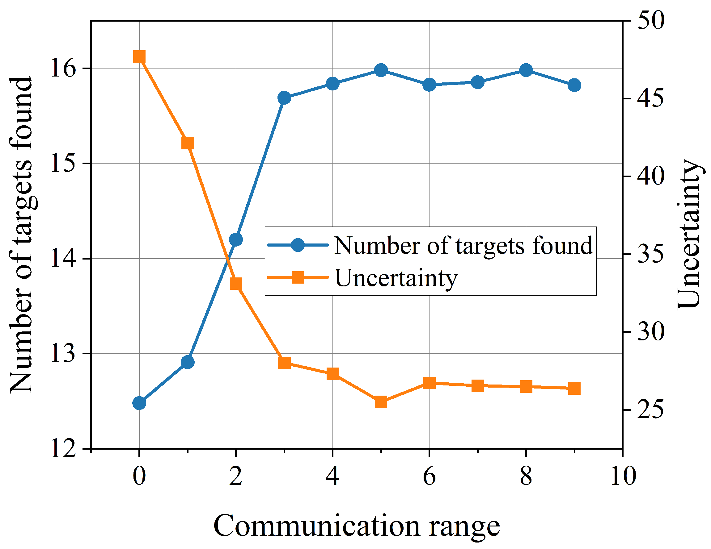
6.2. Communication Model Analysis

To test the effectiveness of the proposed UAV communication and information fusion model, this section analyzes the performance of multi-UAV cooperative reconnaissance under different communication conditions. The communication model was tested using the standard QMIX [31] in a $20\times 20$ map.

Figure 4 shows the distributed uncertainty map U of UAV i under different communication conditions, depicted using contour maps. Redder colors indicate higher uncertainty, while bluer colors indicate lower uncertainty. Compared to heat maps, contour maps more clearly describe the numerical changes in uncertainty across the map. Figure 4a,b shows the uncertainty maps with communication, where UAV i achieves compelling environmental exploration through real-time information sharing. Over time, the overall map becomes bluer, indicating reduced uncertainty. In contrast, Figure 4c,d shows the uncertainty maps without communication, where UAV i is unaware of the reconnaissance results of other UAVs, leaving most of the map red. The scattered blue areas on the right side of the map indicate no-fly zones. Comparing Figure 4a and Figure 4c at the same time shows that UAV i in Figure 4c is likely to continue exploring the red areas already covered by other UAVs, while UAV i in Figure 4a uses the communication mechanism to gain a comprehensive understanding of the entire map, effectively avoiding overlapping trajectories and improving reconnaissance efficiency.

Figure 5 tests the impact of communication distance on the number of targets discovered and the level of uncertainty. As the communication distance increases, the number of targets discovered gradually rises, and uncertainty gradually decreases, eventually converging to a stable value. This indicates that increasing the communication distance enhances information exchange opportunities among UAVs, improving their cooperative reconnaissance and search capabilities. In the $20\times 20$ map, when the communication distance of the UAVs reaches 5, the number of targets discovered and the level of uncertainty have already converged to optimal values, indicating that a larger communication distance is not necessary to achieve the best communication effect.

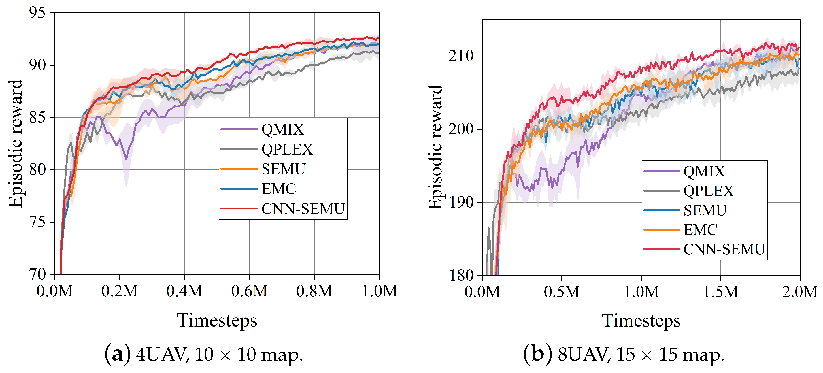
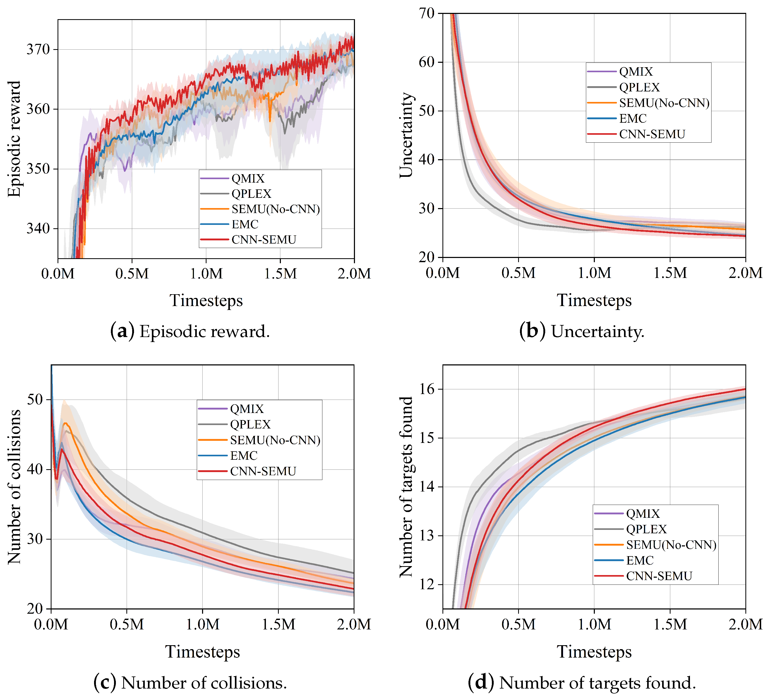
6.3. Baseline Experiment Analysis

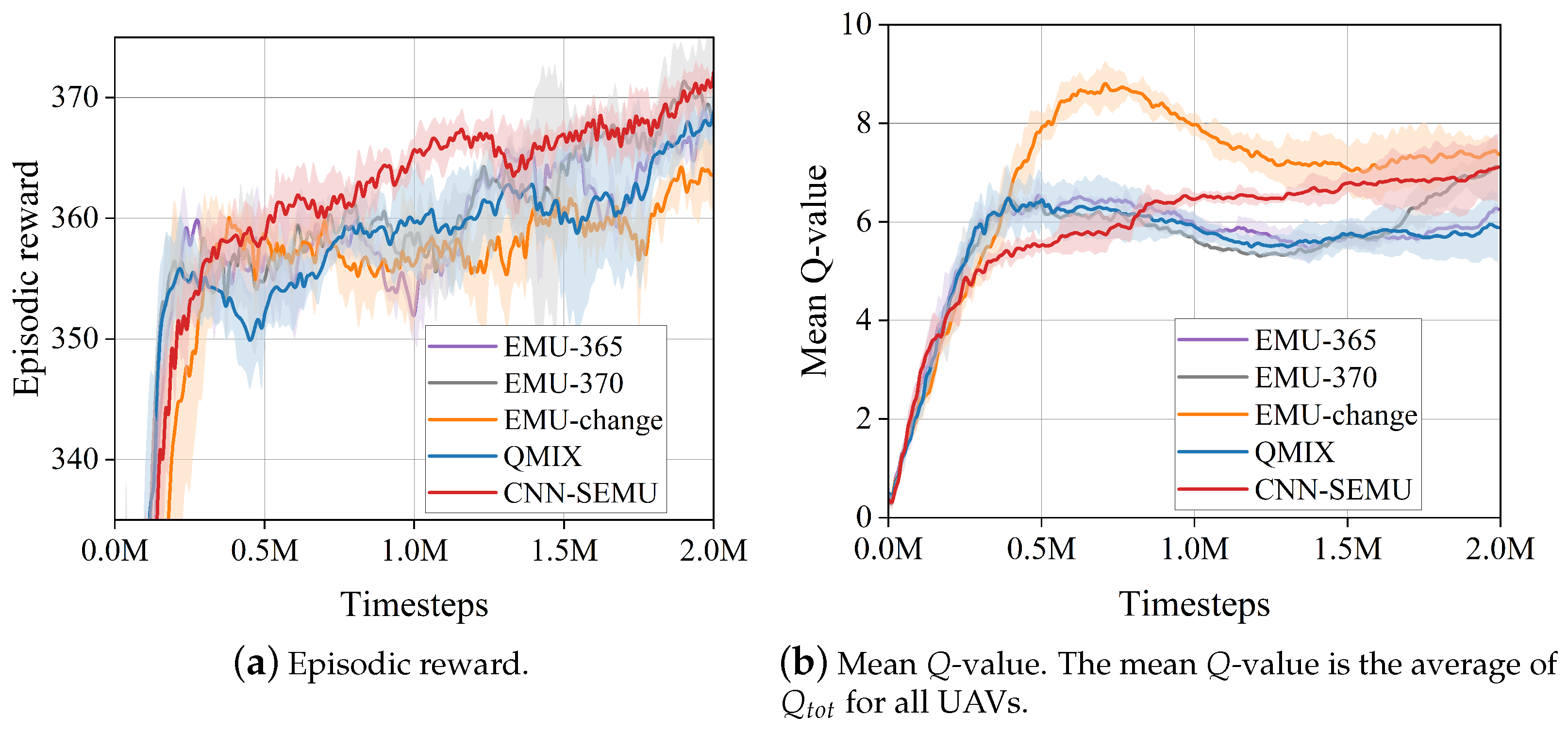
CNN-SEMU can be integrated with any value decomposition-based MADRL framework. In this paper, we implemented CNN-SEMU based on the QMIX algorithm. The experiments compared EMC and EMU, both using QMIX as the basic framework, and included state-of-the-art MADRL algorithms like QMIX and QPLEX as baselines. Additionally, we conducted an ablation study by removing the CNN structure from CNN-SEMU (denoted as SEMU).

Figure 6 compares the episodic rewards of CNN-SEMU and baseline algorithms on $10\times 10$ and $15\times 15$ maps. The results show that CNN-SEMU achieves the best performance in smaller task scenarios.

Figure 7 shows the experimental results of 10 UAVs on $20\times 20$ map. The experiment compared four metrics: episodic reward, uncertainty, number of collisions, and number of targets found. As shown in Figure 7a, CNN-SEMU achieved the best performance, and all three episodic memory-based methods outperformed QMIX and QPLEX, demonstrating the effectiveness of episodic memory. QPLEX had the fastest convergence in uncertainty and the number of targets found in the early stages of training but the slowest convergence in the number of collisions. Additionally, CNN-SEMU converged the fastest and to better values in uncertainty, the number of collisions, and the number of targets found.

Episodic methods improve sampling efficiency by recalling the highest returns of historical states and using one-step memory TD loss to estimate the action–state value function more quickly and accurately. This results in better performance compared to non-episodic QMIX and QPLEX. As shown in Figure 7a, SEMU, which only uses the encoder–decoder structure, performs worse than EMC with random projection in the later stages of training. This is because it is challenging to directly extract features in the high-dimensional (880) map state space. In contrast, CNN-SEMU uses CNN to extract map features, achieving semantically meaningful embeddings that can recall similar states with higher returns. It is worth noting that CNN-SEMU initially performs worse than QMIX in the early stages of training, as the embedding network has not yet captured the important features of the high-dimensional map state space.

Comparison with EMU

EMU also uses an encoder–decoder structure for state embedding. However, unlike the one-step TD memory target, EMU introduces episodic incentives to provide additional rewards for states on desirable trajectories. Episodic incentives are defined as

$$r_p=\gamma {\displaystyle \frac{N_{\xi }\left(s^{\prime }\right)}{N_{call}\left(s^{\prime }\right)}}(H\left(f_{\varphi }\left(s^{\prime }\right)\right)-\underset{a^{\prime }}{max}{Q}_{{\theta }^{-}}(s^{\prime },a^{\prime })),$$

(33)

where $N_{call}\left(s^{\prime }\right)$ represents the total number of times state $s^{\prime }$ is visited in the episodic buffer, and $N_{\xi }\left(s^{\prime }\right)$ represents the number of desirable visits. The final loss function is expressed as

$$\mathcal{L}\left(\theta \right)={\mathbb{E}}_{\tau ,a,r,{\tau }^{\prime }\in \mathcal{D}}\left[{(r_p+y(\tau ,a)-Q_{tot}(\tau ,a;\theta ))}^2\right].$$

(34)

EMU defines desirable trajectories as those with episodic rewards exceeding a preset threshold $R_{\mathrm{thr}}$. In StarCraft II, the maximum reward is obtained when all enemy units are eliminated, and [27] sets this maximum reward as the threshold $R_{\mathrm{thr}}$. For the MCRS-LCR problem, discovering all targets is challenging, making it difficult to determine the maximum overall episodic reward. In the comparative experiments, using a $20\times 20$ map as an example, we set $R_{\mathrm{thr}}$ to 365 and 370 based on the results in Figure 7a. Additionally, we set a periodically updated $R_{\mathrm{thr}}$ that can be adjusted based on the episodic rewards tested during training. This allows states initially deemed desirable to be re-evaluated as undesirable as cognition updates. However, when the desirability of states in the episodic buffer changes, it becomes difficult to determine $N_{\xi }\left(s^{\prime }\right)$. Therefore, we omit $N_{\xi }\left(s^{\prime }\right)/N_{call}\left(s^{\prime }\right)$ from Equation (33) and denote this method as EMU-change.

In the comparative experiments with EMU, we used the same CNN-based embedding structure. As shown in Figure 8a, CNN-SEMU exhibited the best performance, while EMU-365/370 performed similarly to QMIX. This is because EMU only receives episodic incentives when the recalled state is desirable, resulting in EMU-365/370 rarely receiving the $r_p$ signal during training. Figure 8b shows that EMU-365/370 maintains a similar average $Q-value$ to QMIX, indicating that the episodic incentive $r_p$ did not take effect. Figure 8b displays the $Q_{tot}$ average value for all UAVs. It is evident that the EMU-change has a much higher average $Q-value$ than the other algorithms, indicating it received the $r_p$ signal. However, as shown in Figure 8a, the EMU-change performs worse than QMIX. This may be because, although the desirability update enhances the episodic incentive effect, it overestimates the action–state value function. In contrast, CNN-SEMU can quickly and accurately estimate the action-state value function.

6.4. State Embedding Analysis

This subsection examines how the proposed algorithm alters the embedding space, affecting performance. Figure 9 shows the t-SNE [40] visualization results of $20K$ randomly sampled state samples from a $1M$ memory episodic buffer in a $20\times 20$ map task. Since the state vectors have no labels, we label each state vector with its corresponding highest return H.

Figure 9a shows the state vectors before embedding. State vectors with similar colors are clustered together, indicating that state vectors with similar returns are closely arranged in space before embedding. Figure 9b shows the embedded state space using EMC random projection. Although random projection approximately preserves the distance relationships between state vectors, the embedded states are scattered in space with almost no clustering effect. Figure 9c shows the embedding representation of CNN-SEMU without the CNN structure, achieving primary clustering but still less effective than in Figure 9d.

CNN-SEMU achieves good clustering of similar return embeddings, resulting in a smoother embedding space. This indicates that the encoder–decoder with a CNN structure can effectively extract features with reward semantics. Additionally, this clustering makes selecting episodic memory around $x_t$ safer (Figure 3e), ensuring that the memories queried within a certain threshold are closely related states. This allows a larger $\delta$ to be chosen, effectively utilizing more memories.

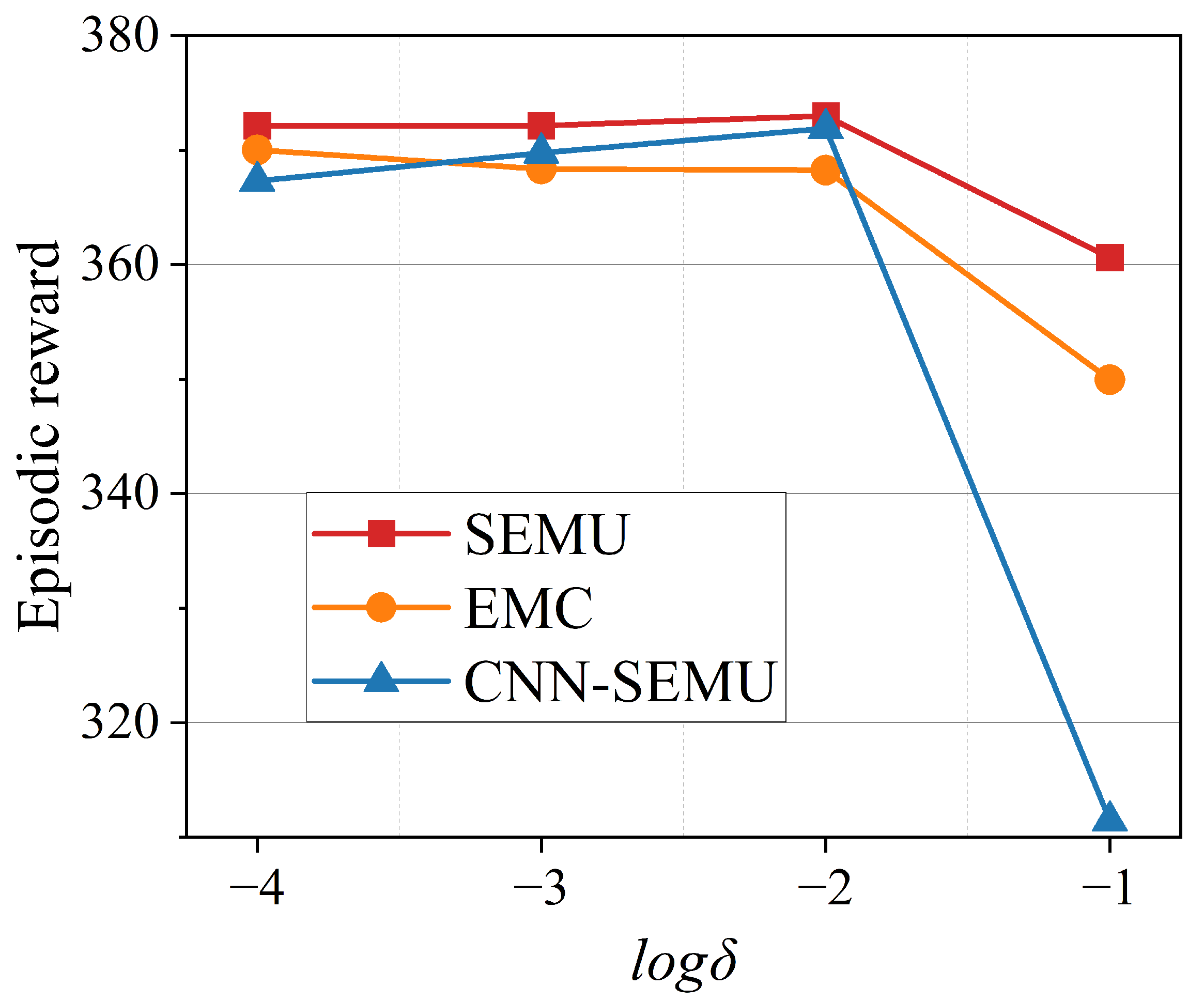
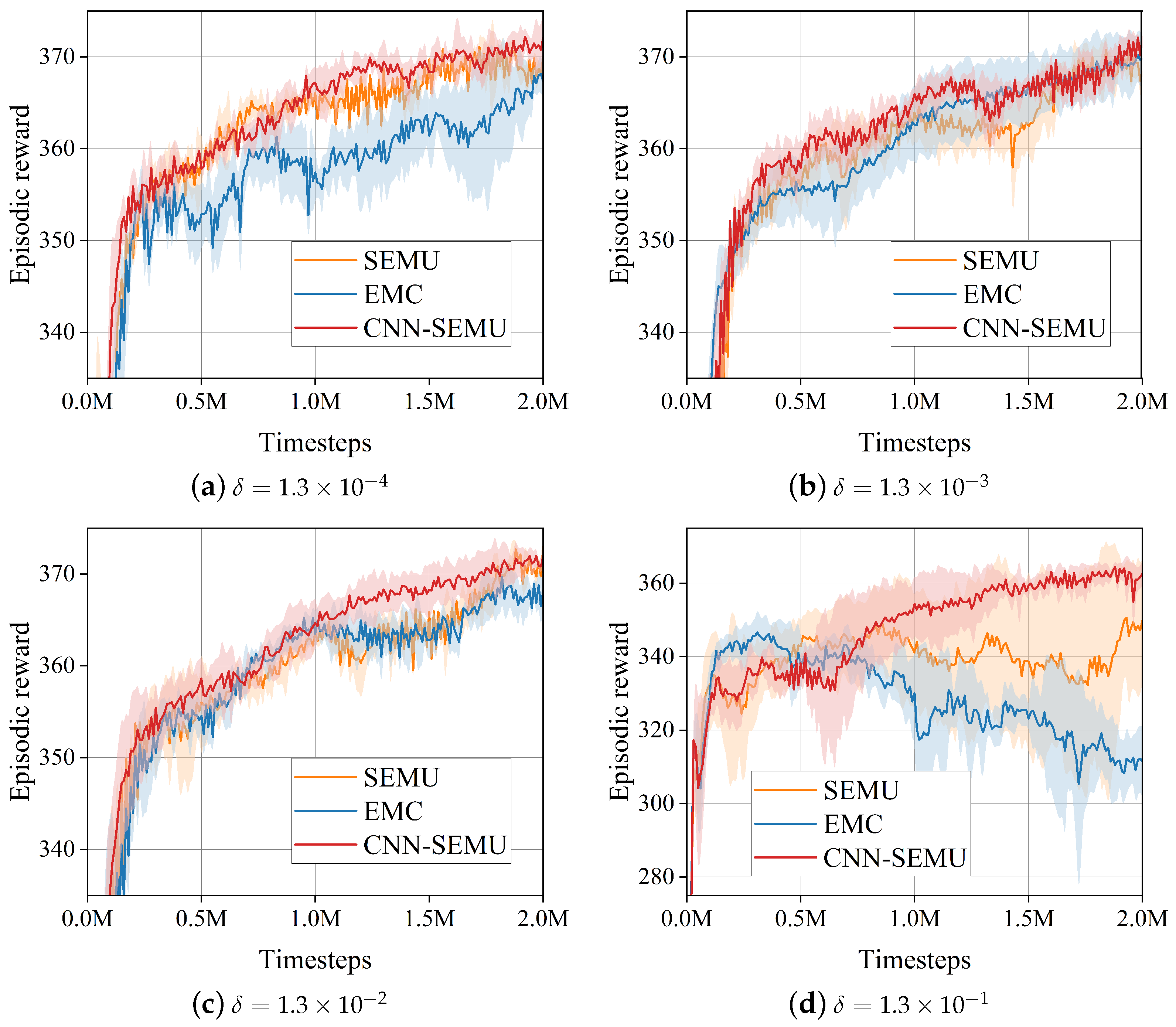
6.5. Hyperparametric Analysis

Selecting appropriate hyperparameters is essential for model training. This section examines the impact of critical hyperparameters $\lambda$ and $\delta$ on algorithm performance. The hyperparameter experiments are conducted using a $20\times 20$ map as an example.

(1) Sensitivity analysis of regularization factor $\lambda$

$\lambda$ controls the proportion of one-step TD memory loss in Equation (32). In this subsection, we examine the stability of CNN-SEMU’s performance under different settings of $\lambda$ ($[0.01,0.05,0.1,0.5,1]$). As shown in Figure 10, when $\lambda$ is 0.01, 0.05, or 0.1, CNN-SEMU achieves optimal performance. However, when $\lambda$ is too large (0.5 or 1), the algorithm’s performance degrades significantly. This may be because excessive recall of historical states causes the algorithm to get stuck in local optima.

(2) Sensitivity analysis of the state-embedding difference threshold $\delta$

$\delta$ influences the update and usage of the episodic buffer during training through Equation (30). In this section, we study the impact of different $\delta$ values on three episodic-based methods: EMC, SEMU, and CNN-SEMU. EMC constructs the embedding space using random projection, CNN-SEMU uses an encoder–decoder structure with CNN, and SEMU is a variant of CNN-SEMU without the CNN structure.

Ref. [27] proposed a method to determine the appropriate threshold $\delta$, expressed as

$$\delta \le {\displaystyle \frac{{(2\times 3{\sigma }_x)}^{dim\left(x\right)}}{M}},$$

(35)

where M is the capacity of the episodic buffer, and ${\sigma }_x$ represents the standard deviation of x in the episodic buffer. When $dim\left(x\right)=4$, $M=1\times {10}^6$, and ${\sigma }_x$ is approximately 1, $\delta$ can be calculated as $\delta \le 0.0013$. Therefore, in this subsection, we set the $\delta$ range to $[1.3\times {10}^{-4},1.3\times {10}^{-3},1.3\times {10}^{-2},1.3\times {10}^{-1}]$ to study its impact on episodic-based methods.

Figure 11 shows the episodic reward at the end of training for different $\delta$ settings, with the horizontal axis on a logarithmic scale. From Figure 11, it is evident that CNN-SEMU achieves the best training performance across various $\delta$ values and performs well over a broader range of $\delta$. When $\delta =1.3\times {10}^{-1}$, the episodic reward for EMC drops sharply. This is because EMC uses random projection to construct the embedding space, resulting in a disordered distribution (as shown in Figure 9b). Within the $\delta =1.3\times {10}^{-1}$ range, it is possible to retrieve states with significantly different reward values, and this excessive recall can disrupt the training process.

To demonstrate both training efficiency and effectiveness,

Table 4. The effect of $\delta$ on episodic reward according to training time.

Timesteps (M)	0.67			1.33			2.00
$\mathit{\delta }$	EMC	SEMU	CNN-SEMU	EMC	SEMU	CNN-SEMU	EMC	SEMU	CNN-SEMU
$1.3\times {10}^{-4}$	355.69	363.22	359.17	360.20	365.63	369.16	367.30	370.01	372.11
$1.3\times {10}^{-3}$	356.03	358.62	361.91	365.62	360.33	363.02	369.75	368.35	372.34
$1.3\times {10}^{-2}$	359.43	358.84	359.77	361.68	361.30	368.24	366.49	369.74	371.91
$1.3\times {10}^{-1}$	339.95	343.10	337.03	321.97	342.96	358.17	311.41	349.96	362.51

The optimal results of each parameter experiment are highlighted in bold.

lists the episodic reward based on training time, and Figure 12 shows the training curves for different $\delta$ values. As shown in Table 4, CNN-SEMU, which uses an encoder–decoder structure with CNN, converges faster and to a higher episodic reward in most cases. This indicates that in the smoother state space constructed by CNN-SEMU, it is safe to retrieve memories from a wider range of $\delta$. However, when $\delta =1.3\times {10}^{-1}$, CNN-SEMU’s performance declines, suggesting that although CNN-SEMU is robust to a wide range of $\delta$, excessively large $\delta$ can still recall completely unrelated states. Therefore, selecting an appropriate $\delta$ helps improve algorithm performance. When $\delta =1.3\times {10}^{-3}$, CNN-SEMU converges to the highest value, indicating that the choice of $\delta$ in Equation (35) is reasonable.

As shown in Figure 12, a larger $\delta$ results in higher episodic reward variance than a smaller $\delta$. When $\delta =1.3\times {10}^{-1}$, both EMC and SEMU fail to find the optimal strategy and exhibit larger error bands, validating our previous analysis. Although larger $\delta$ can recall more similar states, it may also recall completely unrelated states. In contrast, CNN-SEMU uses semantic embedding with CNN, clustering states with the same reward in the embedding space. This makes the space smoother and reduces the likelihood of recalling unrelated states.

7. Conclusions and Future Work

This paper focuses on the multi-UAV cooperative reconnaissance and search problem with a limited communication range (MCRS-LCR) for unknown static targets. We propose a cooperative communication and information fusion model based on belief maps. For the MCRS-LCR problem, we introduce a new multi-agent reinforcement learning method based on episodic memory called CNN-SEMU. CNN-SEMU uses an encoder–decoder structure with CNN to construct the embedding space, extracting high-return semantic features from the high-dimensional map state space, making the embedding space smoother. Ultimately, CNN-SEMU improves reinforcement learning sampling efficiency through one-step memory TD targets, thereby enhancing learning. Extensive baseline simulations demonstrate that CNN-SEMU outperforms state-of-the-art multi-agent reinforcement learning methods in episodic rewards, search efficiency, and collision frequency. State embedding and parameter sensitivity analyses reveal the reasons for CNN-SEMU’s superior performance. This is due to the encoder–decoder with a CNN structure, which achieves better semantic state embeddings.

Future research will optimize communication methods between UAVs to reduce unnecessary load. We will also consider constraints such as communication delay and bandwidth to address practical challenges. Currently, our research focuses on the reconnaissance and search of static targets. Moving forward, we will extend our research to include dynamic target reconnaissance and address the challenges of transitioning from simulation to reality.

References

1. Wu, J.; Sun, Y.; Li, D.; Shi, J.; Li, X.; Gao, L.; Yu, L.; Han, G.; Wu, J. An Adaptive Conversion Speed Q-Learning Algorithm for Search and Rescue UAV Path Planning in Unknown Environments. IEEE Trans. Veh. Technol. 2023, 72, 15391–15404. [Google Scholar] [CrossRef]
2. Li, X.; Lu, X.; Chen, W.; Ge, D.; Zhu, J. Research on UAVs Reconnaissance Task Allocation Method Based on Communication Preservation. IEEE Trans. Consum. Electron. 2024, 70, 684–695. [Google Scholar] [CrossRef]
3. Liu, K.; Zheng, J. UAV Trajectory Optimization for Time-Constrained Data Collection in UAV-Enabled Environmental Monitoring Systems. IEEE Internet Things J. 2022, 9, 24300–24314. [Google Scholar] [CrossRef]
4. Senthilnath, J.; Harikumar, K.; Sundaram, S. Metacognitive Decision-Making Framework for Multi-UAV Target Search without Communication. IEEE Trans. Syst. Man Cybern. Syst. 2024, 54, 3195–3206. [Google Scholar] [CrossRef]
5. Xia, J.; Zhou, Z. The Modeling and Control of a Distributed-Vector-Propulsion UAV with Aero-Propulsion Coupling Effect. Aerospace 2024, 11, 284. [Google Scholar] [CrossRef]
6. Oliehoek, F.A.; Amato, C. A Concise Introduction to Decentralized POMDPs; SpringerBriefs in Intelligent Systems, Springer International Publishing: Cham, Switzerland, 2016. [Google Scholar] [CrossRef]
7. Zhang, B.; Lin, X.; Zhu, Y.; Tian, J.; Zhu, Z. Enhancing Multi-UAV Reconnaissance and Search Through Double Critic DDPG with Belief Probability Maps. IEEE Trans. Intell. Veh. 2024, 9, 3827–3842. [Google Scholar] [CrossRef]
8. Shen, G.; Lei, L.; Zhang, X.; Li, Z.; Cai, S.; Zhang, L. Multi-UAV Cooperative Search Based on Reinforcement Learning with a Digital Twin Driven Training Framework. IEEE Trans. Veh. Technol. 2023, 72, 8354–8368. [Google Scholar] [CrossRef]
9. Yan, K.; Xiang, L.; Yang, K. Cooperative Target Search Algorithm for UAV Swarms with Limited Communication and Energy Capacity. IEEE Commun. Lett. 2024, 28, 1102–1106. [Google Scholar] [CrossRef]
10. Chung, T.H.; Burdick, J.W. Analysis of Search Decision Making Using Probabilistic Search Strategies. IEEE Trans. Rob. 2012, 28, 132–144. [Google Scholar] [CrossRef]
11. Yang, Y.; Polycarpou, M.M.; Minai, A.A. Multi-UAV Cooperative Search Using an Opportunistic Learning Method. J. Dyn. Syst. Meas. Contr. 2007, 129, 716–728. [Google Scholar] [CrossRef]
12. Liu, S.; Yao, W.; Zhu, X.; Zuo, Y.; Zhou, B. Emergent Search of UAV Swarm Guided by the Target Probability Map. Appl. Sci. 2022, 12, 5086. [Google Scholar] [CrossRef]
13. Zhang, C.; Zhou, W.; Qin, W.; Tang, W. A novel UAV path planning approach: Heuristic crossing search and rescue optimization algorithm. Expert Syst. Appl. 2023, 215, 119243. [Google Scholar] [CrossRef]
14. Yue, W.; Xi, Y.; Guan, X. A New Searching Approach Using Improved Multi-Ant Colony Scheme for Multi-UAVs in Unknown Environments. IEEE Access 2019, 7, 161094–161102. [Google Scholar] [CrossRef]
15. Zhang, W.; Zhang, W. An Efficient UAV Localization Technique Based on Particle Swarm Optimization. IEEE Trans. Veh. Technol. 2022, 71, 9544–9557. [Google Scholar] [CrossRef]
16. Mnih, V.; Kavukcuoglu, K.; Silver, D.; Rusu, A.A.; Veness, J.; Bellemare, M.G.; Graves, A.; Riedmiller, M.; Fidjeland, A.K.; Ostrovski, G.; et al. Human-level control through deep reinforcement learning. Nature 2015, 518, 529–533. [Google Scholar] [CrossRef]
17. Samvelyan, M.; Rashid, T.; De Witt, C.S.; Farquhar, G.; Nardelli, N.; Rudner, T.G.J.; Hung, C.M.; Torr, P.H.S.; Foerster, J.; Whiteson, S. The StarCraft multi-agent challenge. In Proceedings of the International Joint Conference on Autonomous Agents and Multiagent Systems, AAMAS, Montreal, Canada, 13–17 May 2019; Volume 4, pp. 2186–2188. [Google Scholar]
18. Wang, Y.; Zhang, J.; Chen, Y.; Yuan, H.; Wu, C. An Automated Learning Method of Semantic Segmentation for Train Autonomous Driving Environment Understanding. IEEE Trans. Ind. Inf. 2024, 20, 6913–6922. [Google Scholar] [CrossRef]
19. Li, J.; Liu, Q.; Chi, G. Distributed deep reinforcement learning based on bi-objective framework for multi-robot formation. Neural Netw. 2024, 171, 61–72. [Google Scholar] [CrossRef] [PubMed]
20. Bellemare, M.G.; Naddaf, Y.; Veness, J.; Bowling, M. The Arcade Learning Environment: An evaluation platform for general agents. J. Artif. Intell. Res. 2013, 47, 253–279. [Google Scholar] [CrossRef]
21. Squire, L.R. Memory systems of the brain: A brief history and current perspective. Neurobiol. Learn. Mem. 2004, 82, 171–177. [Google Scholar] [CrossRef]
22. Biane, J.S.; Ladow, M.A.; Stefanini, F.; Boddu, S.P.; Fan, A.; Hassan, S.; Dundar, N.; Apodaca-Montano, D.L.; Zhou, L.Z.; Fayner, V.; et al. Neural dynamics underlying associative learning in the dorsal and ventral hippocampus. Nat. Neurosci. 2023, 26, 798–809. [Google Scholar] [CrossRef]
23. Turner, V.S.; O’Sullivan, R.O.; Kheirbek, M.A. Linking external stimuli with internal drives: A role for the ventral hippocampus. Curr. Opin. Neurobiol. 2022, 76, 102590. [Google Scholar] [CrossRef]
24. Eichenbaum, H. Prefrontal–hippocampal interactions in episodic memory. Nat. Rev. Neurosci. 2017, 18, 547–558. [Google Scholar] [CrossRef] [PubMed]
25. Blundell, C.; Uria, B.; Pritzel, A.; Li, Y.; Ruderman, A.; Leibo, J.Z.; Rae, J.; Wierstra, D.; Hassabis, D. Model-free episodic control. arXiv 2016, arXiv:1606.04460. [Google Scholar]
26. Zheng, L.; Chen, J.; Wang, J.; He, J.; Hu, Y.; Chen, Y.; Fan, C.; Gao, Y.; Zhang, C. Episodic Multi-agent Reinforcement Learning with Curiosity-driven Exploration. Adv. Neural Inf. Process. Syst. 2021, 5, 3757–3769. [Google Scholar]
27. Na, H.; Seo, Y.; Moon, I.C. Efficient episodic memory utilization of cooperative multi-agent reinforcement learning. arXiv 2024, arXiv:2403.01112. [Google Scholar]
28. Ma, X.; Li, W.J. State-based episodic memory for multi-agent reinforcement learning. Mach. Learn. 2023, 112, 5163–5190. [Google Scholar] [CrossRef]
29. Lin, Z.; Zhao, T.; Yang, G.; Zhang, L. Episodic memory deep q-networks. In Proceedings of the Twenty-Seventh International Joint Conference on Artificial Intelligence, IJCAI, Stockholm, Sweden, 13–19 July 2018; Volume 2018-July, pp. 2433–2439. [Google Scholar] [CrossRef]
30. Johnson, W.B.; Lindenstrauss, J.; Schechtman, G. Extensions of Lipschitz maps into Banach spaces. Isr. J. Math. 1986, 54, 129–138. [Google Scholar] [CrossRef]
31. Rashid, T.; Samvelyan, M.; De Witt, C.S.; Farquhar, G.; Foerster, J.; Whiteson, S. QMIX: Monotonic value function factorisation for deep multi-agent reinforcement Learning. In Proceedings of the International Conference on Machine Learning (ICML 2018), Stockholm, Sweden, 10–15 July 2018; Volume 10, pp. 6846–6859. [Google Scholar]
32. Wang, J.; Ren, Z.; Liu, T.; Yu, Y.; Zhang, C. QPLEX: Duplex Dueling Multi-Agent Q-Learning. arXiv 2020, arXiv:2008.01062. [Google Scholar]
33. Azzam, R.; Boiko, I.; Zweiri, Y. Swarm Cooperative Navigation Using Centralized Training and Decentralized Execution. Drones 2023, 7, 193. [Google Scholar] [CrossRef]
34. Khan, A.A.; Adve, R.S. Centralized and distributed deep reinforcement learning methods for downlink sum-rate optimization. IEEE Trans. Wireless Commun. 2020, 19, 8410–8426. [Google Scholar] [CrossRef]
35. Son, K.; Kim, D.; Kang, W.J.; Hostallero, D.; Yi, Y. QTRAN: Learning to factorize with transformation for cooperative multi-agent reinforcement learning. In Proceedings of the International Conference on Machine Learning, ICML 2019, Long Beach, CA, USA, 9–15 June 2019; Volume 2019-June, pp. 10329–10346. [Google Scholar]
36. Sunehag, P.; Lever, G.; Gruslys, A.; Czarnecki, W.M.; Zambaldi, V.; Jaderberg, M.; Lanctot, M.; Sonnerat, N.; Leibo, J.Z.; Tuyls, K.; et al. Value-decomposition networks for cooperative multi-agent learning based on team reward. In Proceedings of the International Joint Conference on Autonomous Agents and Multiagent Systems, AAMAS, Stockholm, Sweden, 10–15 July 2018; Volume 3, pp. 2085–2087. [Google Scholar]
37. Wang, M.; Xu, X.; Yue, Q.; Wang, Y. A comprehensive survey and experimental comparison of graph-based approximate nearest neighbor search. Proc. VLDB Endow. 2021, 14, 1964–1978. [Google Scholar] [CrossRef]
38. Liu, Q.; Zhou, S. LightFusion: Lightweight CNN Architecture for Enabling Efficient Sensor Fusion in Free Road Segmentation of Autonomous Driving. IEEE Trans. Circuits Syst. II Express Briefs 2024. early access. [Google Scholar] [CrossRef]
39. Zhang, Y.; Wilker, K. Visual-and-Language Multimodal Fusion for Sweeping Robot Navigation Based on CNN and GRU. J. Organ. End User Comput. 2024, 36, 1–21. [Google Scholar] [CrossRef]
40. Van der Maaten, L.; Hinton, G. Visualizing data using t-SNE. J. Mach. Learn. Res. 2008, 9, 2579–2605. [Google Scholar]
Figure 1. An example of episodic memory is a child’s encounter with an ice cream truck, a highly rewarding experience. When the child hears the truck’s music, they recall the previous scene of buying ice cream, including the music (a), the park location (b), the queue of customers (c), and the truck itself (d). The brain constructs episodic memories by recognizing these key features and associating them with positive experiences, guiding the child’s behavior, such as running outside when the music is heard.
Drones 08 00393 g001
Figure 2. System model: UAVs have eight possible movement directions. They coordinate reconnaissance and target search through a limited communication range with other UAVs while avoiding no-fly zones.
Drones 08 00393 g002
Figure 3. An overview of CNN-SEMU. (a) Standard value factorization CTDE framework. (b) Replay buffer. (c) Episodic buffer. (d) State embedding module. (e) Scenario memory utilization. (f) CNN structure.
Drones 08 00393 g003
Figure 4. Distributed uncertainty map U of UAV i under different communication conditions.
Drones 08 00393 g004
Figure 5. The effect of the communication range on the number of targets found and the uncertainty.
Drones 08 00393 g005
Figure 6. Comparison of CNN-SEMU and baseline algorithms on episodic reward.
Drones 08 00393 g006
Figure 7. Performance comparison of CNN-SEMU and baseline algorithms on 20 × 20 Map.
Drones 08 00393 g007
Figure 8. Performance comparison of CNN-SEMU and EMU.
Drones 08 00393 g008
Figure 9. Visualization of embedded and original states sampled from D E using t-SNE. The rainbow-colored circles, from red to purple, represent embedded states with low to high reward values.
Drones 08 00393 g009
Figure 10. The effect of hyperparameter λ on CNN-SEMU performance.
Drones 08 00393 g010
Figure 11. Episodic reward at the end of training for different values of δ .
Drones 08 00393 g011
Figure 12. The effect of δ on episodic reward.
Drones 08 00393 g012