A Robust Hybrid Iterative Learning Formation Strategy for Multi-Unmanned Aerial Vehicle Systems with Multi-Operating Modes

Abstract

This paper investigates the formation control problem of multi-unmanned aerial vehicle (UAV) systems with multi-operating modes. While mode switching enhances the flexibility of multi-UAV systems, it also introduces dynamic model switching behaviors in UAVs. Moreover, obtaining an accurate dynamic model for a multi-UAV system is challenging in practice. In addition, communication link failures and time-varying unknown disturbances are inevitable in multi-UAV systems. Hence, to overcome the adverse effects of the above challenges, a hybrid iterative learning formation control strategy is proposed in this paper. The proposed controller does not rely on precise modeling and exhibits its learning ability by utilizing historical input–output data to update the current control input. Furthermore, two convergence theorems are proven to guarantee the convergence of state, disturbance estimation, and formation tracking errors. Finally, three simulation examples are conducted for a multi-UAV system consisting of four quadrotor UAVs under multi-operating modes, switching topologies, and external disturbances. The results of the simulations show the strategy’s effectiveness and superiority in achieving the desired formation control objectives.

1. Introduction

In recent years, unmanned aerial vehicles (UAVs), which are aircraft capable of autonomous flight and load-carrying, have garnered significant attention from researchers in both the scientific and engineering communities. Compared to the single UAV systems, multi-UAV systems composed of groups of homogeneous/heterogeneous UAVs have the advantage of collaborative task execution and a wide range of applications in complex task scenarios [1], such as multi-satellite systems [2], persistent reconnaissance [3,4], and cargo transportation [5]. Formation control, one of the most fundamental coordinating control problems of multi-UAV systems [6,7], entails ensuring that any neighboring UAVs keep a fixed deviation while tracking the desired trajectory. Hitherto, several formation keeping methods have been well studied, including behavioral-based methods [8], artificial potential field methods [9], and distributed leader–follower methods [10,11]. Additionally, as a typical model-free intelligent algorithm, reinforcement learning is also widely used in motion planning and formation problems of multi-UAV systems [12,13]. Specifically, the design of leader–follower formation control for multi-UAV systems depends on a well-constructed communication graph, where each UAV can only interact with its neighboring UAVs [14].

For the control problem of leader–follower formation tracking, numerous researchers have proposed a variety of control algorithms, considering UAVs’ dynamic models to be nonlinear, strongly coupled, time-varying, and underactuated. In [15], Gong et al. present an event-triggered distributed formation algorithm, which, compared to centralized algorithms, facilitates the more efficient and flexible task execution of multi-satellite systems. In [11], a neural adaptive sliding mode controller is proposed to address the uncertainty and unmodeled dynamic models of multi-UAV systems. In [16], the optimization control technique is utilized in the design of a distributed leader–follower formation tracking scheme, and in [17], for multi-UAV systems subject to multi-constraints, a model predictive control scheme is proposed to achieve a formation flight. Additionally, a recurrent neural network-based leader–follower consensus formation control method for small-size nonlinear UAVs is presented in [18]. Based on the aforementioned methods for multi-UAV systems and considering the conservation of communication resources, the distributed formation control method is generally regarded as efficient because it requires information only from local neighboring UAVs rather than all UAVs [19].

However, in certain application scenarios, UAVs must switch between different operating modes to adapt to various working environments. For example, an amphibious robot described in [20] is designed with multi-mode operations to work flexibly in different environments, such as beaches, grasslands, seabeds, and underwater. In [21], the researchers present a novel self-reconfigurable modular robotic system with multi-mode locomotion and conduct an experiment with two locomotion modes: inchworm-type mode and quadruped-walker mode. In [22], the researchers develop a soft crawling robot with three locomotive modes (inchworm-like motion, creeping, and tumbling) to enhance the locomotion ability of untethered robots in narrow spaces. Therefore, this paper considers a class of multi-UAV systems composed of the individual UAVs with multi-operating modes, such as those described in [20,21], and it significantly enhances the application potential of multi-UAV systems in diverse working environments. Additionally, in [23], the dynamical system with multi-operating modes is described as a switched dynamic system consisting of a finite number of sub-modes, and such switching behavior complicates the designs of formation control algorithms of multi-UAV systems with multi-operating modes.

Meanwhile, the switching behaviors, resulting from the communication link failures or cyber-attacks, may occur in the communication topology, and many researchers have studied the formation control of multi-UAV systems with switching communication topologies. For instance, in [24], Zou et al. assume that the switching topologies are uniformly jointly connected, and design an adaptive controller to address the formation tracking of multiple vertical takeoff and landing UAVs. In [25], the inner–outer distributed second-order controller is presented for the formation tracking of multi-rotors under switching topologies with velocities and acceleration saturation constraints. In [26], under Markovian random switching topologies, a distributed formation control strategy combining the unknown parameter observer is put forward for a group of quadrotor UAVs. However, up to now, no literature has been found that addresses multi-UAV systems with multi-operating modes and switching communication topologies.

In addition, most existing formation tracking studies [26,27] are valid in the infinity time domain. However, this characteristic also imposes limitations on dealing with finite-time practical tasks. Unlike other control algorithms that investigate the convergence/stability of controlled systems in the infinite time domain, iterative learning control (ILC)-based methods aim to improve the tracking performance of repetitive dynamic systems in the iteration domain by learning from previous iterations. In [28], the researchers design a double proportional–derivative-type (PD-type) ILC control strategy for leader–follower formation tracking of a class of linear multiple quadrotor UAV systems. For the nonlinear and non-affine multi-UAV systems, Fu et al. use a data-driven ILC with a dynamic linearization approximation approach to handle the point–point leader–follower formation tracking problem in [29]. In [30], a derivative-type (D-type) ILC-based leader–follower formation control algorithm is constructed for a team of quadrotors. However, existing ILC-based formation control schemes [29,30] are difficult to apply to multi-UAV systems with multi-operating modes due to the presence of switching operating modes.

Motivated by the preceding discussions, we focus on an application scenario of repeat cargo transportation of multi-UAV systems. Thus, UAVs are required to have the ability to carry cargoes, and each UAV has two operating modes: on-load mode (i.e., the UAV is working under carrying cargoes), and no-load mode (i.e., the UAV is working without carrying cargoes). However, some dynamic parameters, including total mass, center of mass, and rotational inertia, undergo substantial variations when releasing heavy payloads. Developing a dynamic model to encompass various payload scenarios and designing a single flight controller throughout the mission are highly challenging [31]. Thus, a class of multi-UAV systems with multi-operating modes are considered. This paper investigates a hybrid iterative learning formation strategy for multi-UAV systems under multi-operating modes, switching communication topologies and unknown external disturbances. The contributions and novelty of this paper are summarized as follows.

• We propose a hybrid robust iterative learning formation control strategy that combines a state and disturbance iterative learning observer (ILO), and an iterative learning controller for multi-UAV systems under multi-operating modes. In contrast to the existing literature on formation control for multi-UAV systems [32,33], this paper extends the application fields of multi-UAV system formation control from the single operating mode to the multi-operating mode.
• The proposed method does not depend on the accurate dynamic model of multi-UAV systems, and the control input in the current iteration is updated by utilizing the stored data from previous iterations.
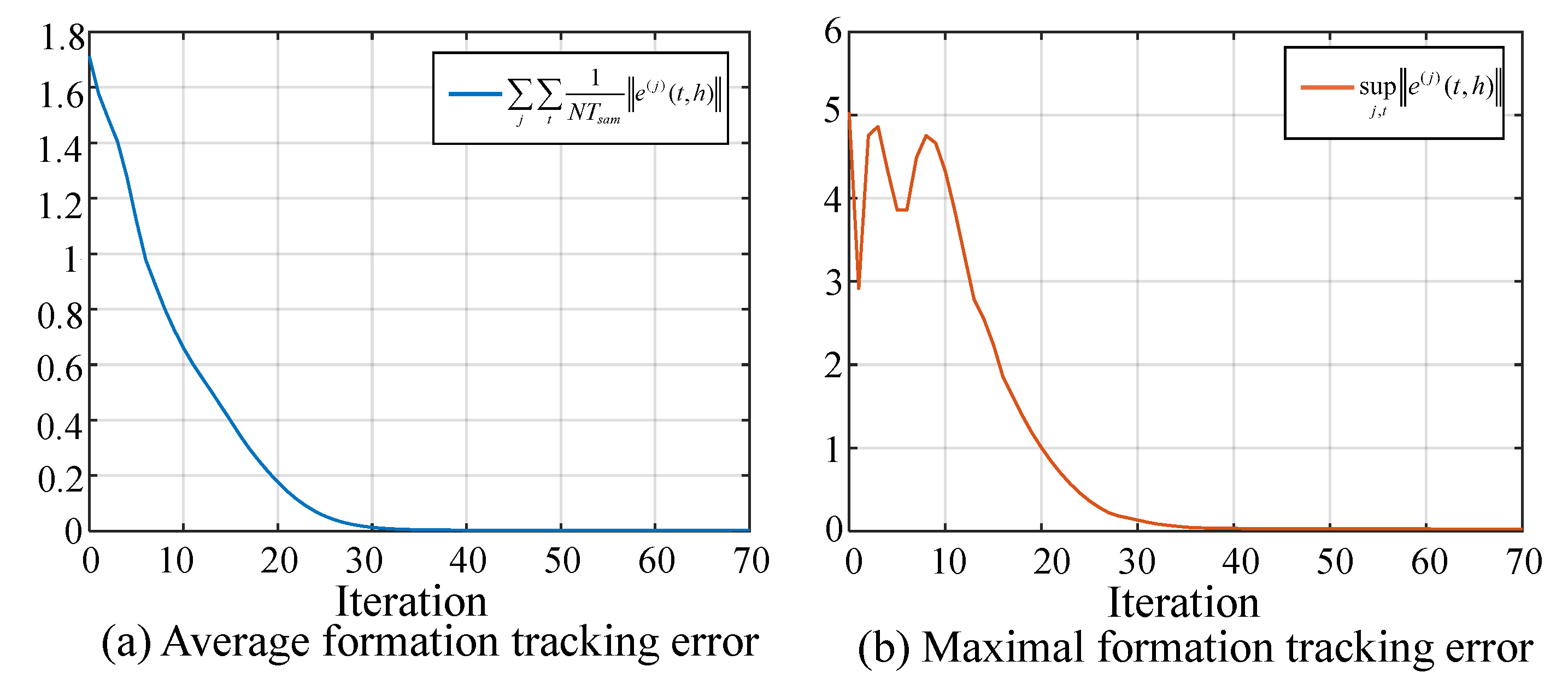
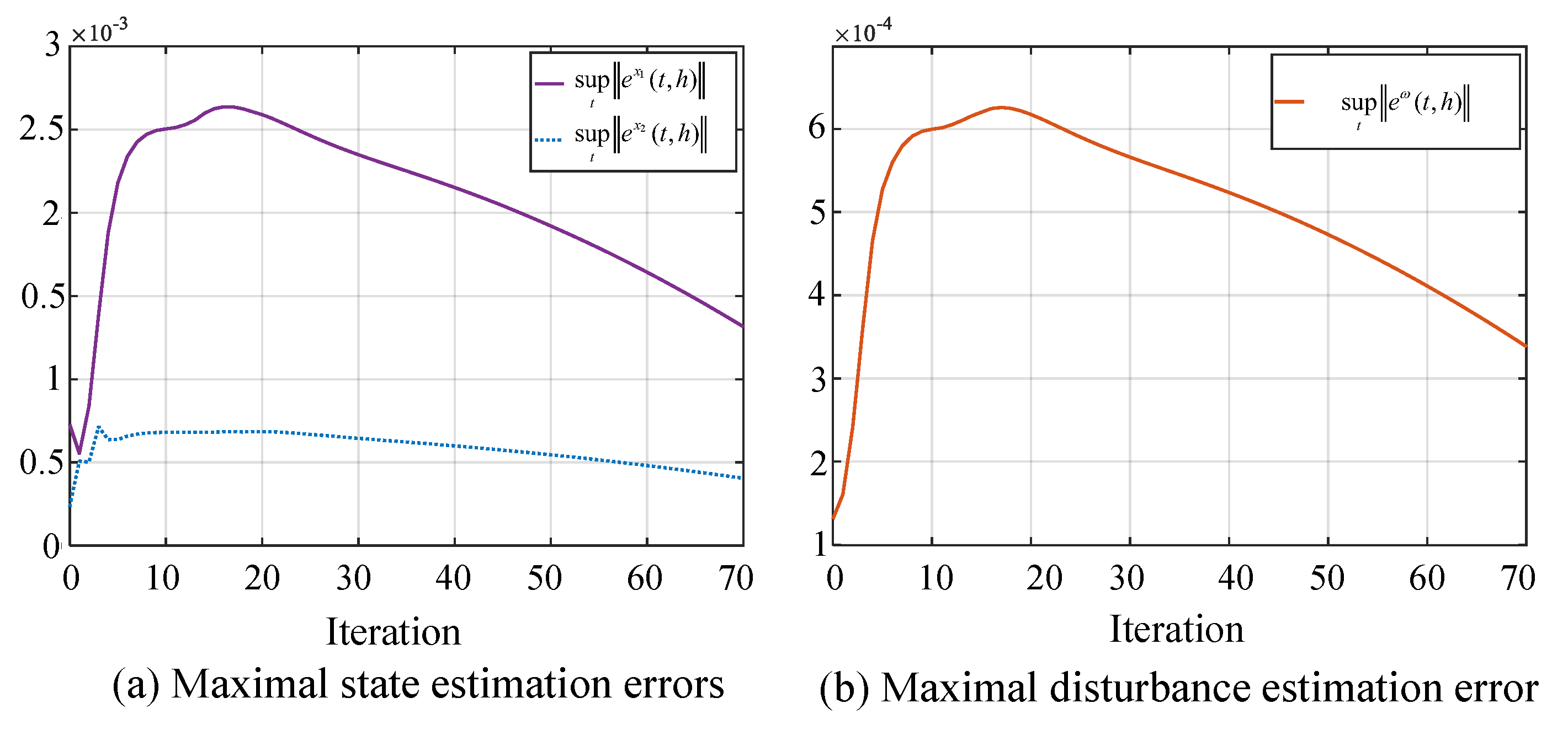
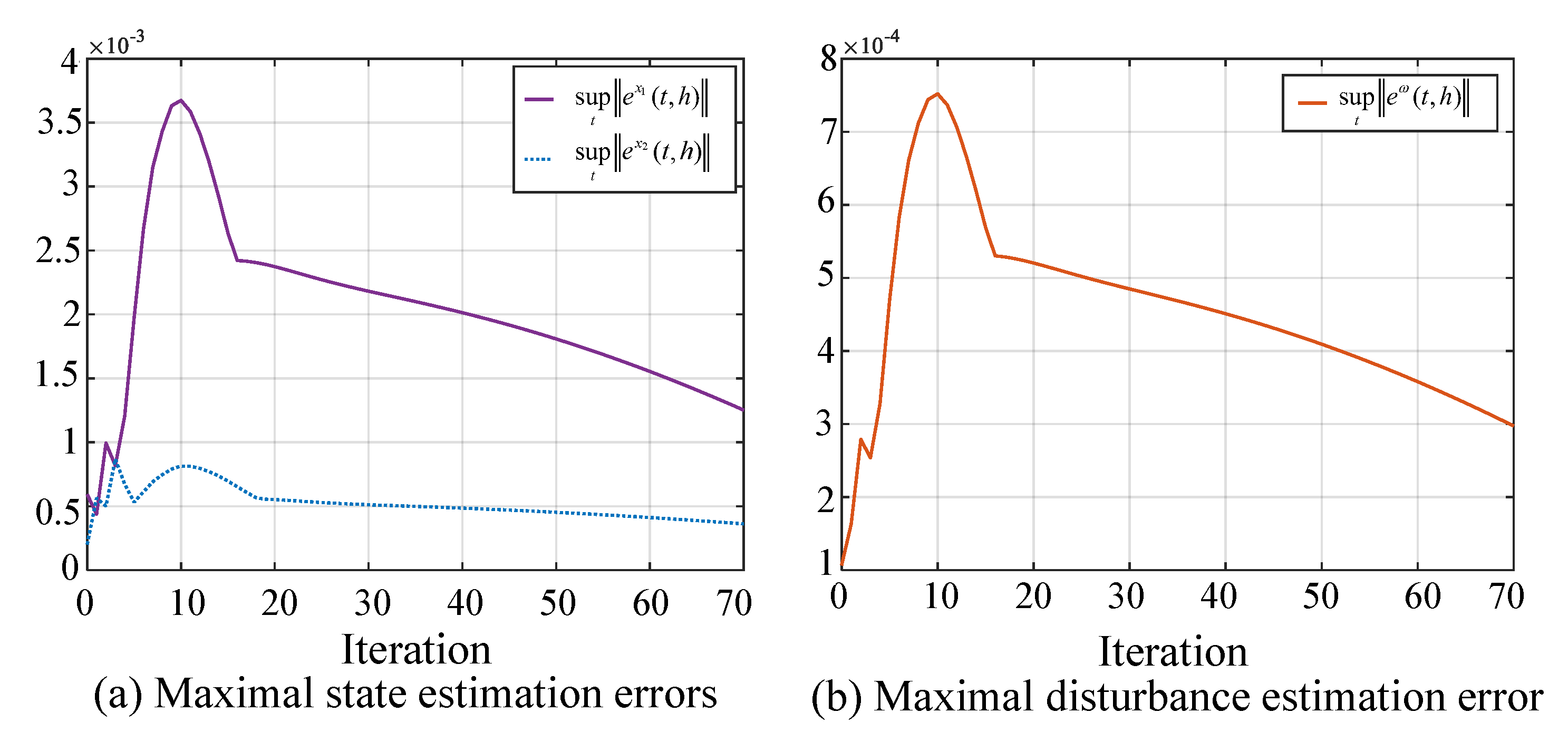
• Compared to iterative learning works for multi-UAV systems [28,29], an iteration-fixed initial state assumption is not required in this paper. Detailed theoretical results are described to ensure the convergence of state and disturbance estimated errors and the formation tracking error with the proposed hybrid formation control strategy.
• Three simulation experiments with a multi-UAV system composed of four quadrotor UAVs are conducted to demonstrate the effectiveness and the superiority of the proposed formation strategy in dealing with the finite-time formation tracking.

The rest of this paper is structured as follows. Section 2 presents the communication topology theory and the general second-order nonlinear dynamic model of multi-UAV systems, along with the key assumptions and lemmas. Section 3 proposes the hybrid iterative learning formation control strategy, and the detailed theoretical results are presented in Section 4. The simulation is conducted in Section 5 and Section 6, concluding the paper.

Notation 1.

“⊗” denotes the Kronecker product. $\parallel a\parallel$ and $\parallel A\parallel$ are the vector norm and matrix norm, respectively. $I_n=diag\{1,1,\dots ,1\}$, $1_n={\{1,1,\dots ,1\}}^T$ and ${\mathbf{0}}_n={\{0,0,\dots ,0\}}^T$. $A\prec B$ denotes the matrix ($A-B$) is negative-definite. ${\mathbb{Z}}^{+}$ is the set of all non-negative integers. For two vectors $a=(a_1,a_2,a_3)\in {\mathbb{R}}^n$ and $b=(b_1,b_2,b_3)\in {\mathbb{R}}^n$, their cross product is $a\times b=(a_2{b}_3-a_3{b}_2,a_3{b}_1-a_1{b}_3,a_1{b}_2-a_2{b}_1)\in {\mathbb{R}}^n$.

2. Problem Formulation

In this section, we offer some prerequisite knowledge of communication graph and formulate the dynamic model of multi-UAV systems under multi-operating modes.

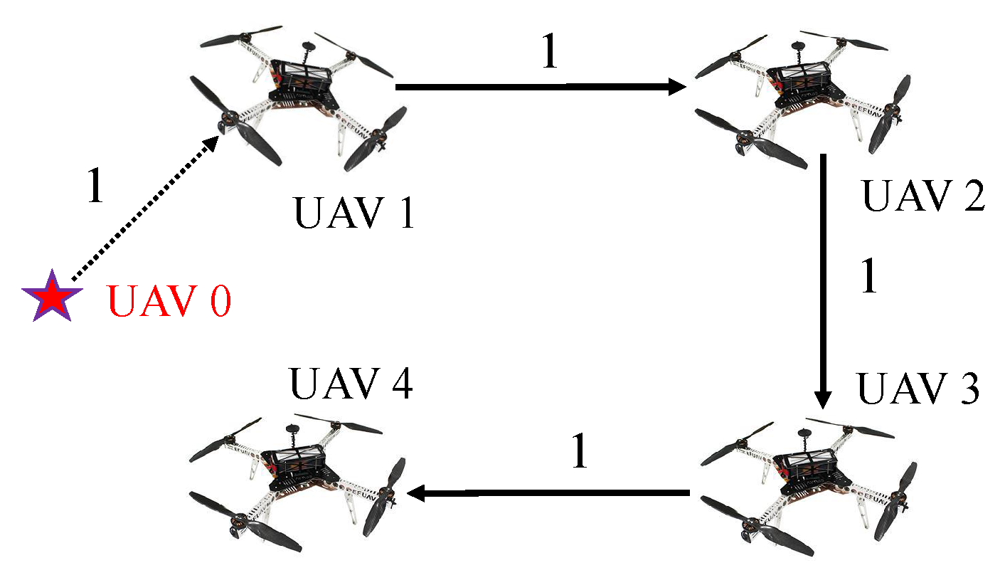
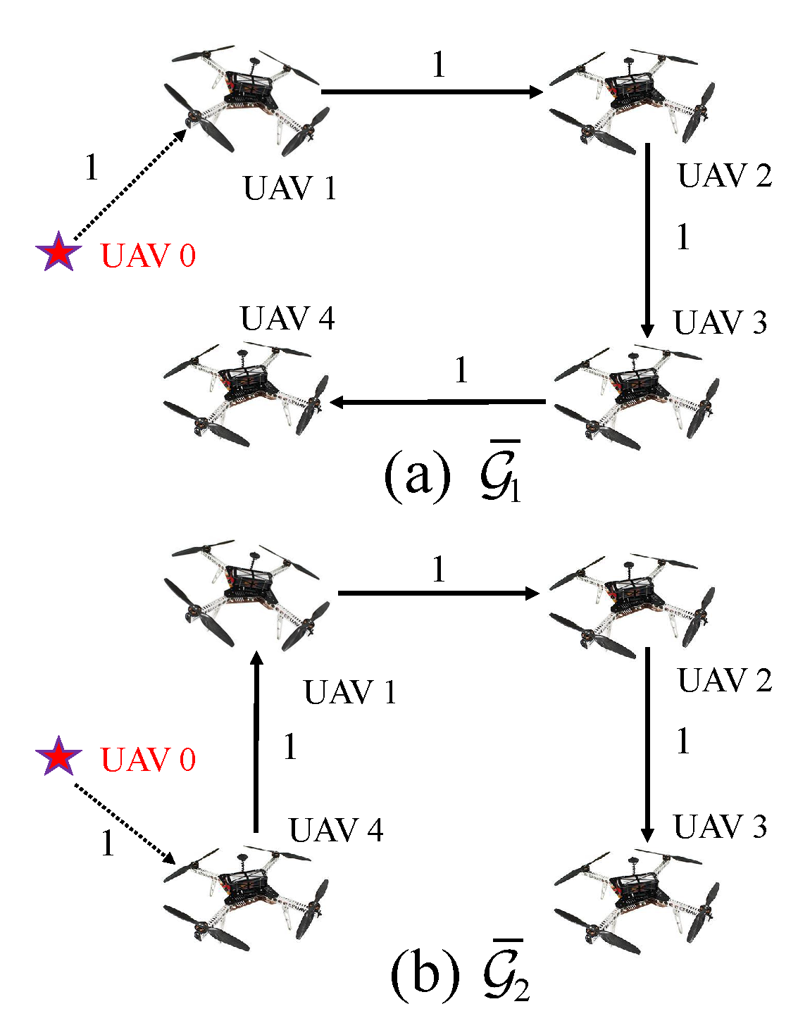
2.1. Communication Topology

A directed graph reflects the connection relationships among UAVs, and is defined by $\mathcal{G}=\{\mathcal{V},\mathcal{E},\mathcal{A}\}$, where $\mathcal{V}=\{v_1,v_2,\dots ,v_N\}$ is the vertex set, $\mathcal{E}$ is the edge set, and $\mathcal{A}$ is the adjacent matrix. If the edge $(j,i)$ belongs to $\mathcal{E}$, then $a^{\left(ij\right)}>0$; otherwise, $a^{\left(ij\right)}=0$. In particular, $a^{\left(ii\right)}=0$. A Laplacian matrix is defined as $\mathcal{L}=(\mathcal{D}-\mathcal{A})\in {\mathbb{R}}^{N\times N}$, where $\mathcal{D}=diag\{{\alpha }^{\left(1\right)},{\alpha }^{\left(2\right)},\dots ,{\alpha }^{\left(N\right)}\}\in {\mathbb{R}}^{N\times N}$ with ${\alpha }^{\left(i\right)}={\sum }_{j=1}^N{a}^{\left(ij\right)}$. In this paper, suppose that the desired trajectory is generated by a leader UAV, and only a portion of the UAVs can exchange information with the leader UAV. Thus, we define $\Pi =diag({\pi }_1,{\pi }_2,\dots ,{\pi }_N)\in {\mathbb{R}}^{N\times N}$ to denote the connection between the UAVs and leader. The graph with a leader UAV is $\overline{\mathcal{G}}=\{\mathcal{V}\cup \left\{0\right\},\overline{\mathcal{E}},\overline{\mathcal{A}}\}$. Then, if all UAVs can form a spanning tree with the leader UAV as the root vertex, this means that the graph $\overline{\mathcal{G}}$ contains a spanning tree.

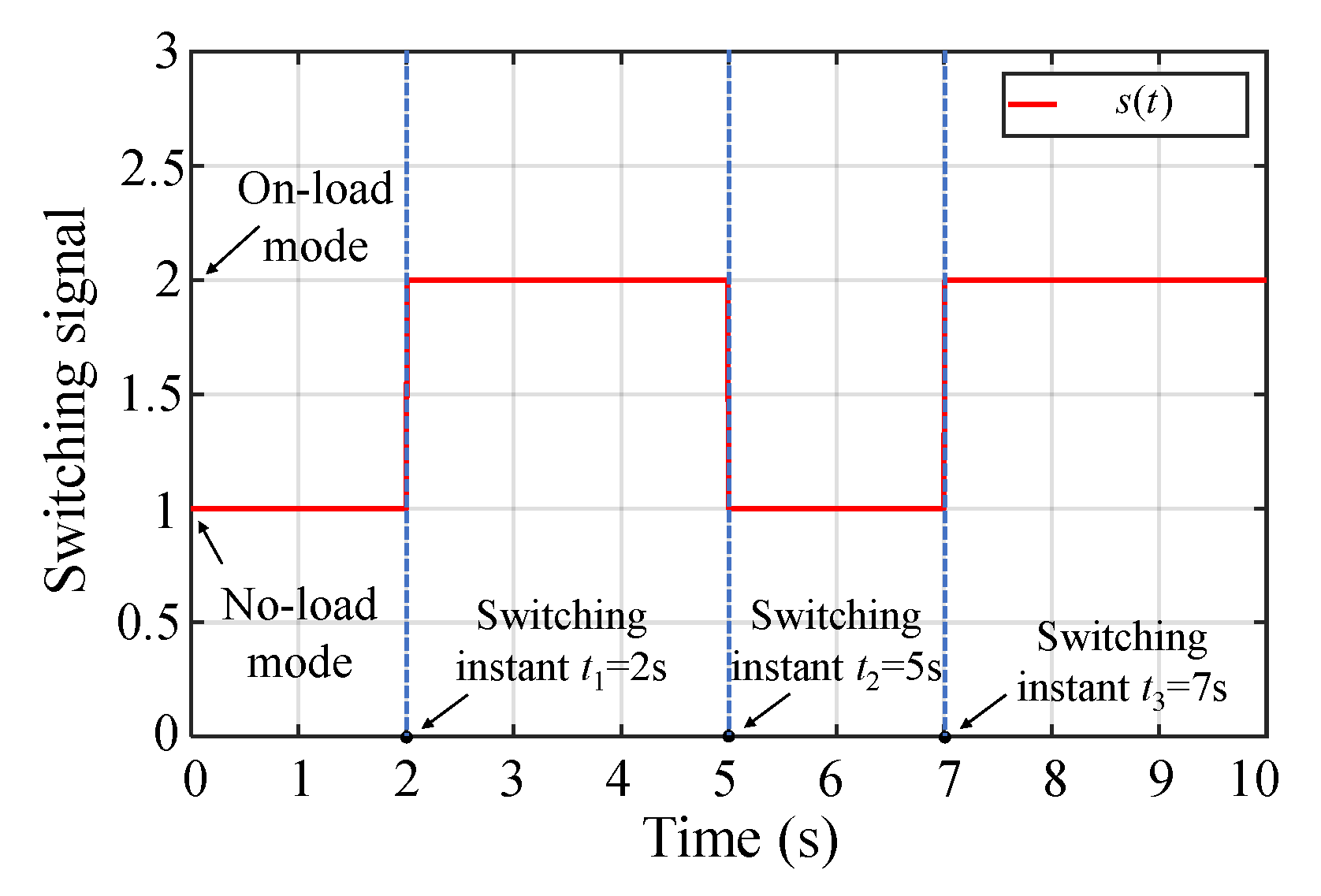
2.2. Multi-UAV Systems with Multi-Operating Modes

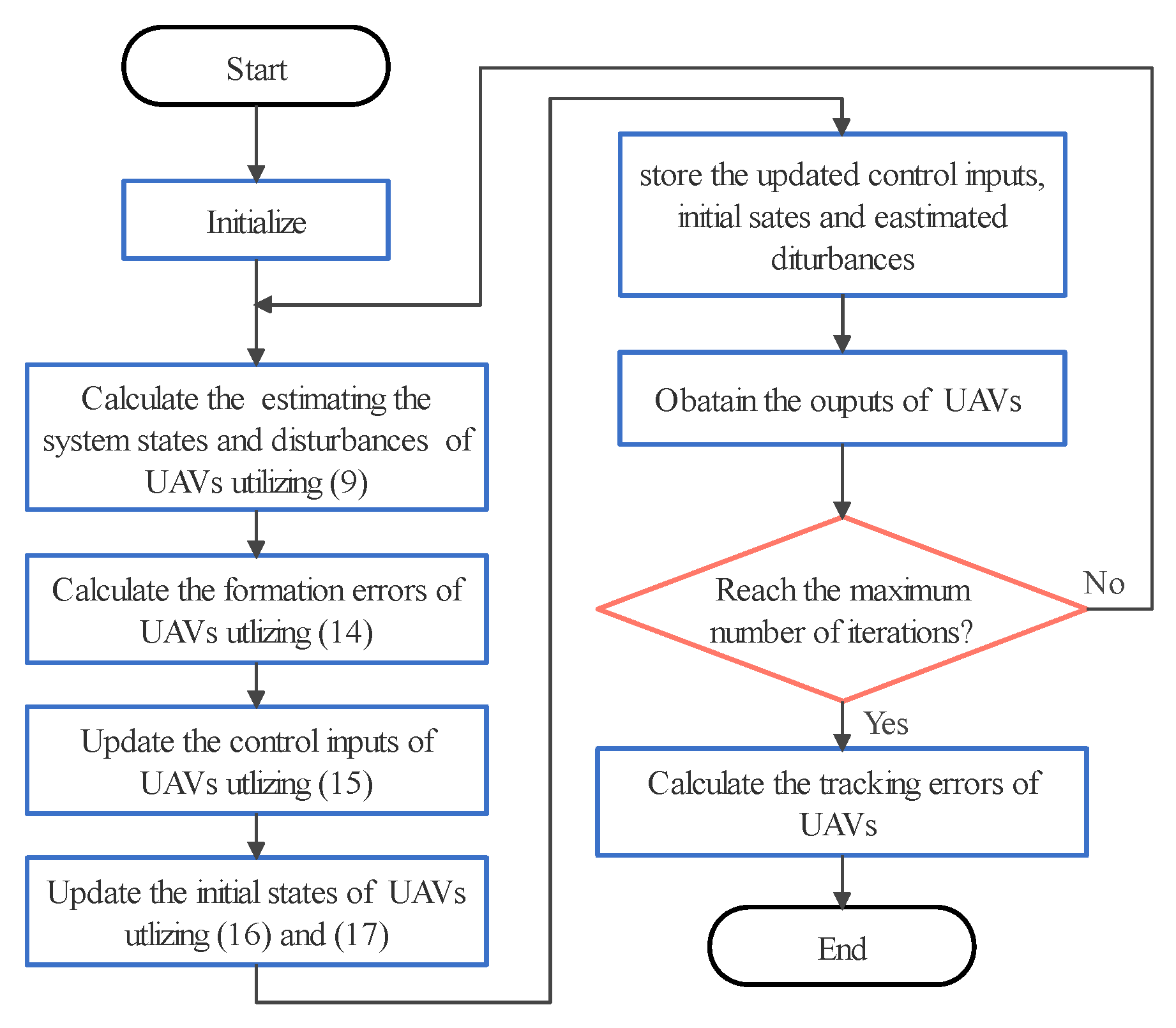
In practical scenarios, the dynamic models of many UAV systems can be described as second-order dynamical systems.Hence, considering the formation tracking issue of multi-UAV systems under multi-operating modes, a general class of second-order nonlinear dynamic models of the j-th UAV at the h-th iteration is expressed as

$$\begin{array}{c}\hfill \left\{\begin{array}{cc}& {\dot{x}}_1^{\left(j\right)}(t,h)=x_2^{\left(j\right)}(t,h)\hfill \\ & {\dot{x}}_2^{\left(j\right)}(t,h)=f_{s\left(t\right)}\left(x_2^{\left(j\right)}(t,h)\right)+B_{s\left(t\right)}{u}^{\left(j\right)}(t,h)+{\omega }_{s\left(t\right)}^{\left(j\right)}(t,h)\hfill \\ & y^{\left(j\right)}(t,h)=C_{s\left(t\right)}{x}_1^{\left(j\right)}(t,h)\hfill \end{array}\right.\end{array}$$

(1)

where $t\in [0,T]$, $h\in {\mathbb{Z}}^{+}$ is the iteration number, and $j\in \{1,2,\dots ,N\}$. ${x_1}^{\left(j\right)}(t,h),{x_2}^{\left(j\right)}(t,h)\in {\mathbb{R}}^n$, $u^{\left(j\right)}(t,h)\in {\mathbb{R}}^p$ and $y^{\left(j\right)}(t,h)\in {\mathbb{R}}^m$ are the state, input, and output of the UAV. ${{\dot{x}}_1}^{\left(j\right)}(t,h),{{\dot{x}}_2}^{\left(j\right)}(t,h)\in {\mathbb{R}}^n$ are first-order time derivatives of ${x_1}^{\left(j\right)}(t,h),{x_2}^{\left(j\right)}(t,h)$. $B_{s\left(t\right)}\in {\mathbb{R}}^{n\times p}$ is a full-of-row rank input matrix and $C_{s\left(t\right)}\in {\mathbb{R}}^{m\times n}$ is an output matrix. $f_{s\left(t\right)}\left({x_2}^{\left(j\right)}(t,h)\right):{\mathbb{R}}^n\to {\mathbb{R}}^n$ is a vector-valued nonlinear function. ${\omega }_{s\left(t\right)}^{\left(j\right)}(t,h)\in {\mathbb{R}}^n$ is a time- and iterative-variant finite external disturbance, and $\parallel {\omega }_{s\left(t\right)}^{\left(j\right)}(t,h)\parallel \le b_{\omega }$, where the positive constant $b_{\omega }$ is a finite bound. $s\left(t\right)\in \{1,2,...,M\}$ is the operating mode switching law; e.g., if $t\in {\Theta }_k=[t_{k-1},t_k)$, $s\left(t\right)=k$.

Remark 1.

For the multi-UAV system (1), the system matrices and vectors exhibit a switching behavior in different operating modes. However, the switching behavior, resulting from communication link failures or cyber-attacks, may occur in the communication topology, referred to as the switching topology ${\overline{\mathcal{G}}}_{s\left(t\right)}\in \{{\overline{\mathcal{G}}}_1,{\overline{\mathcal{G}}}_2,\dots ,{\overline{\mathcal{G}}}_M\}$, and its corresponding Laplacian matrix is $L_{s\left(t\right)}$. In particular, any sub-topology ${\overline{\mathcal{G}}}_k$, ($k\in \{1,2,\dots ,M\}$) can form a spanning tree and the leader is the root vertex.

Here, some assumptions and lemmas contributing to the analysis are firstly given.

Assumption A1.

For any $t\in {\Theta }_k$, the nonlinear function $f_k\left(·\right)$ is assumed to be differentiable with respect to the state x and satisfies the Lipschitz condition $\parallel f_k\left(\tilde{x}\right)-f_k\left(\widehat{x}\right)\parallel \le l_f\parallel \tilde{x}-\widehat{x}\parallel$, where constant $l_f>0$ is the Lipschitz constant.

Remark 2.

Assumption 1 is to provide some prior knowledge for the unknown nonlinear term $f_k\left(·\right)$ of the multi-UAV system (1), and many practical networked systems are considered to be composed of nonlinear individuals that satisfy Assumption 1, e.g., [34,35].

Lemma 1

([36]). The non-negative real sequences $\left\{r_h\right\}\in \mathbb{R}$ and $\left\{q_h\right\}\in \mathbb{R}$ satisfy $r_{h+1}\le ϵr_h+q_h$; if the positive constant $ϵ<1$ and ${lim}_{h\to \infty }{q}_h=q_{\infty }$, then we have ${lim}_{h\to \infty }{r}_h\le q_{\infty }/(1-ϵ)$.

Lemma 2

([37]). For a vector-valued function $f\left(t\right)\in {\mathbb{R}}^n$, where $t\in {\Theta }_k$, its λ-norm is defined by ${\parallel f\left(·\right)}_{{\Theta }_k}{\parallel }_{\lambda }={sup}_{t\in {\Theta }_k}exp(-\lambda t)\parallel f\left(t\right)\parallel$. The following two properties associated with λ-norm are valid, i.e.,

(1) For vector-valued functions $f\left(t\right),g\left(t\right)\in {\mathbb{R}}^n$, if $f\left(t\right)={\int }_{t_{k-1}}^{t}g\left(\tau \right)\mathrm{d}\tau$, then

$$\begin{array}{cc}\hfill & {\parallel f\left(·\right)}_{{\Theta }_k}{\parallel }_{\lambda }\le {\displaystyle \frac{1-exp(-\lambda (t_k-t_{k-1}))}{\lambda }}{\parallel g{\left(·\right)}_{{\Theta }_k}\parallel }_{\lambda }\hfill \end{array}$$

(2)

(2) For vector-valued functions $f\left(t\right),g\left(t\right)\in {\mathbb{R}}^n$, if $f\left(t\right)={\int }_{t_{k-1}}^t{\int }_{t_{k-1}}^{s}g\left(\tau \right)\mathrm{d}\tau$, then

$$\begin{array}{cc}\hfill & {\parallel f\left(·\right)}_{{\Theta }_k}{\parallel }_{\lambda }\le {\displaystyle \frac{{(1-exp(-\lambda (t_k-t_{k-1})))}^2}{{\lambda }^2}}{\parallel g{\left(·\right)}_{{\Theta }_k}\parallel }_{\lambda }\hfill \end{array}$$

(3)

Formation objective: Let $d_j\left(t\right)\in {\mathbb{R}}^m$ be the desired formation deviation between the j-th UAV and the virtual leader UAV, and let $d_{jl}\left(t\right)=d_j\left(t\right)-d_l\left(t\right)\in {\mathbb{R}}^m$ be the desired formation deviation between the j-th UAV and the l-th UAV. For the multi-UAV system (1) with multi-operating modes under the switching law $s\left(t\right)$, and with both the switching communication topology and unknown external disturbance being considered, the formation objective is to design an appropriate control input $u^{\left(j\right)}(t,h)$ such that each each UAV maintains a desired deviation from its neighbor UAVs over a finite time interval [38], i.e.,

$$\begin{array}{cc}\hfill & \underset{h\to +\infty }{lim}(y^{\left(i\right)}(t,h)-y^{\left(j\right)}(t,h))=d_{ij}\left(t\right),i,j\in \mathcal{V},i\ne j.\hfill \end{array}$$

(4)

Then, we define a leader trajectory tracking error as $e^{\left(j\right)}(t,h)=y_d\left(t\right)+d_j\left(t\right)-y^{\left(j\right)}(t,h)$. It is noted that the control objective (4) can be ensured if the formation tracking error $e^{\left(j\right)}(t,h)$ is convergent in the iteration domain. In order to facilitate the analysis later, for any $t\in {\Theta }_k$, the compact form of the multi-UAV system (1) is denoted by

$$\begin{array}{c}\hfill \left\{\begin{array}{cc}& {\dot{x}}_1(t,h)=x_2(t,h)\hfill \\ & {\dot{x}}_2(t,h)=f_k\left(x_2(t,h)\right)+{\tilde{B}}_{k}u(t,h)+{\omega }_k(t,h)\hfill \\ & y(t,h)={\tilde{C}}_k{x}_1(t,h)\hfill \end{array}\right.\end{array}$$

(5)

where $x_1(t,h)={[x_1^{\left(1\right)}{(t,h)}^{\mathrm{T}},\dots ,x_1^{\left(N\right)}{(t,h)}^{\mathrm{T}}]}^{\mathrm{T}}\in {\mathbb{R}}^{Nn}$, $x_2(t,h)={[x_2^{\left(1\right)}{(t,h)}^{\mathrm{T}},\dots ,x_2^{\left(N\right)}{(t,h)}^{\mathrm{T}}]}^{\mathrm{T}}$$\in {\mathbb{R}}^{Nn}$, $u(t,h)=[u^{\left(1\right)}{(t,h)}^{\mathrm{T}},$$\dots ,u^{\left(N\right)}{(t,h)}^{\mathrm{T}}{]}^{\mathrm{T}}\in {\mathbb{R}}^{Np}$, $y(t,h)={[y^{\left(1\right)}{(t,h)}^{\mathrm{T}},\dots ,y^{\left(N\right)}{(t,h)}^{\mathrm{T}}]}^{\mathrm{T}}$$\in {\mathbb{R}}^{Nm}$. $f_k\left(x_2(t,h)\right)=[f_k{\left(x_2^{\left(1\right)}(t,h)\right)}^{\mathrm{T}},\dots ,$$f_k{\left(x_2^{\left(N\right)}(t,h)\right)}^{\mathrm{T}}{]}^{\mathrm{T}}\in {\mathbb{R}}^{Nn}$. ${\omega }_k(t,h)=[{\omega }_k^{\left(1\right)}{(t,h)}^{\mathrm{T}},$$\dots ,$${\omega }_k^{\left(N\right)}{(t,h)}^{\mathrm{T}}{]}^{\mathrm{T}}\in {\mathbb{R}}^{Nn}$. ${\tilde{B}}_k=I_N\otimes B_k$ and ${\tilde{C}}_k=I_N\otimes C_k$. Thus, the compact form of the tracking error is $e(t,h)=1_N\otimes y_d\left(t\right)+d\left(t\right)-y(t,h)$, where $d\left(t\right)={[d_1{\left(t\right)}^{\mathrm{T}},\dots ,d_N{\left(t\right)}^{\mathrm{T}}]}^{\mathrm{T}}$.

3. Methodology

To achieve the formation tracking of multi-UAV systems under switching dynamic modes, switching communication topologies, and external disturbances, this section proposes a hybrid iterative learning formation strategy.

3.1. ILO Design for Multi-UAV Systems

Due to the unmeasurable states and unknown disturbances in the multi-UAV system (1), a hybrid ILO for estimating the system states and disturbances is proposed as

$$\begin{array}{c}\hfill \left\{\begin{array}{cc}& {{\dot{\widehat{x}}}_1}^{\left(j\right)}(t,h)={{\widehat{x}}_2}^{\left(j\right)}(t,h)\hfill \\ & {{\dot{\widehat{x}}}_2}^{\left(j\right)}(t,h)=f_{s\left(t\right)}\left({{\widehat{x}}_2}^{\left(j\right)}(t,h)\right)+B_{s\left(t\right)}{u}^{\left(j\right)}(t,h)+{\widehat{\omega }}_{s\left(t\right)}^{\left(j\right)}(t,h)+K_{s\left(t\right)}^{\left(j\right)}(y^{\left(j\right)}(t,h)-{\widehat{y}}^{\left(j\right)}(t,h))\hfill \\ & {\widehat{y}}^{\left(j\right)}(t,h)=C_{s\left(t\right)}{\widehat{x}}_1^{\left(j\right)}(t,h)\hfill \\ & {\widehat{\omega }}_{s\left(t\right)}^{\left(j\right)}(t,h+1)={\widehat{\omega }}_{s\left(t\right)}^{\left(j\right)}(t,h)+L_{s\left(t\right)}^{\left(j\right)}({\ddot{y}}^{\left(j\right)}(t,h)-{\ddot{\widehat{y}}}^{\left(j\right)}(t,h))\hfill \end{array}\right.\end{array}$$

(6)

where ${\widehat{x}}_1^{\left(j\right)}(t,h)\in {\mathbb{R}}^n$, ${\widehat{x}}_2^{\left(j\right)}(t,h)\in {\mathbb{R}}^n$, ${\widehat{y}}^{\left(j\right)}(t,h)\in {\mathbb{R}}^m$, and ${\widehat{\omega }}_{s\left(t\right)}^{\left(j\right)}(t,h)\in {\mathbb{R}}^n$ are the estimated state, output, and disturbance vectors, respectively. ${{\dot{\widehat{x}}}_1}^{\left(j\right)}(t,h),{{\dot{\widehat{x}}}_2}^{\left(j\right)}(t,h)\in {\mathbb{R}}^n$ are the first-order time derivatives of ${{\widehat{x}}_1}^{\left(j\right)}(t,h),{{\widehat{x}}_2}^{\left(j\right)}(t,h)$. ${\ddot{y}}^{\left(j\right)}(t,h),{\ddot{\widehat{y}}}^{\left(j\right)}(t,h)\in {\mathbb{R}}^m$ are the second-order time derivatives of $y^{\left(j\right)}(t,h),{\widehat{y}}^{\left(j\right)}(t,h)$. $K_{s\left(t\right)}^{\left(j\right)}\in {\mathbb{R}}^{n\times m}$ and $L_{s\left(t\right)}^{\left(j\right)}\in {\mathbb{R}}^{n\times m}$ are the observer gain matrices. The deviation between the initial estimation states and real states are assumed to be finite, i.e., $\parallel x_1^{\left(j\right)}(0,h)-{\widehat{x}}_1^{\left(j\right)}(0,h)\parallel \le b_{x_1}$ and $\parallel x_2^{\left(j\right)}(0,h)-{\widehat{x}}_2^{\left(j\right)}(0,h)\parallel \le b_{x_2}$.

For any $t\in {\Theta }_k$, the compact form of ILO (6) is

$$\begin{array}{c}\hfill \left\{\begin{array}{cc}& {\dot{\widehat{x}}}_1(t,h)={\widehat{x}}_2(t,h)\hfill \\ & {\dot{\widehat{x}}}_2(t,h)=f_k\left({\widehat{x}}_2(t,h)\right)+{\tilde{B}}_{k}u(t,h)+{\widehat{\omega }}_{s\left(t\right)}(t,h)+K_k(y(t,h)-\widehat{y}(t,h))\hfill \\ & \widehat{y}(t,h)={\tilde{C}}_k{\widehat{x}}_1(t,h)\hfill \\ & {\widehat{\omega }}_k(t,h+1)={\widehat{\omega }}_k(t,h)+L_k(\ddot{y}(t,h)-\ddot{\widehat{y}}(t,h))\hfill \end{array}\right.\end{array}$$

(7)

where ${\widehat{x}}_1(t,h)={[{\widehat{x}}_1^{\left(1\right)}{(t,h)}^{\mathrm{T}},\dots ,{\widehat{x}}_1^{\left(N\right)}{(t,h)}^{\mathrm{T}}]}^{\mathrm{T}}\in {\mathbb{R}}^{N{n}_1}$, ${\widehat{x}}_2(t,h)={[{\widehat{x}}_2^{\left(1\right)}{(t,h)}^{\mathrm{T}},\dots ,{\widehat{x}}_2^{\left(N\right)}{(t,h)}^{\mathrm{T}}]}^{\mathrm{T}}$$\in {\mathbb{R}}^{N{n}_2}$, $\widehat{y}(t,h)=[{\widehat{y}}^{\left(1\right)}{(t,h)}^{\mathrm{T}},$$\dots ,{\widehat{y}}^{\left(N\right)}{(t,h)}^{\mathrm{T}}{]}^{\mathrm{T}}\in {\mathbb{R}}^{Nm}$, and ${\widehat{\omega }}_k(t,h)=[{\widehat{\omega }}_k^{\left(1\right)}{(t,h)}^{\mathrm{T}},\dots ,$${\widehat{\omega }}_k^{\left(N\right)}{(t,h)}^{\mathrm{T}}{]}^{\mathrm{T}}\in {\mathbb{R}}^{Nn}$. $K_k=diag\{K_k^{\left(1\right)},\dots ,K_k^{\left(N\right)}\}$ and $L_k=diag\{L_k^{\left(1\right)},\dots ,L_k^{\left(N\right)}\}$.

The estimated state error and disturbance error are defined as

$$\begin{array}{cc}\hfill & e^{x_1}(t,h)=x_1(t,h)-{\widehat{x}}_1(t,h)\hfill \end{array}$$

(8)

$$\begin{array}{cc}\hfill & e^{x_2}(t,h)=x_2(t,h)-{\widehat{x}}_2(t,h)\hfill \end{array}$$

(9)

$$\begin{array}{cc}\hfill & e_{s\left(t\right)}^{\omega }(t,h)={\omega }_{s\left(t\right)}(t,h)-{\widehat{\omega }}_{s\left(t\right)}(t,h)\hfill \end{array}$$

(10)

3.2. ILC Controller Design for Multi-UAV Systems

The distributed formation tracking error of a multi-UAV system (1) is defined as

$$\begin{array}{cc}\hfill {\psi }^{\left(j\right)}(t,h)=& \sum _{i=1}^N\left(a_{s\left(t\right)}^{\left(ij\right)}(y^{\left(i\right)}(t,h)-y^{\left(j\right)}(t,h)+d_{ji}\left(t\right))\right)+{\pi }_{s\left(t\right)}^{\left(j\right)}(y_d\left(t\right)+d_j\left(t\right)-y^{\left(j\right)}(t,h))\hfill \end{array}$$

(11)

where $a_{s\left(t\right)}^{\left(ij\right)}$ is the element of adjacent matrix ${\mathcal{A}}_{s\left(t\right)}\in {\mathbb{R}}^{N\times N}$, and ${\pi }_{s\left(t\right)}^{\left(j\right)}$ is the diagonal element of the leader connected status matrix ${\Pi }_{s\left(t\right)}\in {\mathbb{R}}^{N\times N}$. Then, a distributed ILC control algorithm is proposed as

$$\begin{array}{cc}\hfill u^{\left(j\right)}(t,h+1)& =u^{\left(j\right)}(t,h)+K_{j,s\left(t\right)}^x{\widehat{\eta }}^{\left(j\right)}(t,h)+{\Lambda }_{j,s\left(t\right)}{\dot{\psi }}^{\left(j\right)}(t,h)+{\Gamma }_{j,s\left(t\right)}{\ddot{\psi }}^{\left(j\right)}(t,h)\hfill \\ \hfill & +K_{j,s\left(t\right)}^{\omega }{\tilde{\widehat{\omega }}}_{s\left(t\right)}^{\left(j\right)}(t,h)\hfill \end{array}$$

(12)

where ${\widehat{\eta }}^{\left(j\right)}(t,h)={\widehat{x}}^{\left(j\right)}(t,h+1)-{\widehat{x}}^{\left(j\right)}(t,h)\in {\mathbb{R}}^n$ and ${\tilde{\widehat{\omega }}}_{s\left(t\right)}^{\left(j\right)}(t,h)={\widehat{\omega }}_{s\left(t\right)}^{\left(j\right)}(t,h+1)-{\widehat{\omega }}_{s\left(t\right)}^{\left(j\right)}(t,h)$$\in {\mathbb{R}}^n$. ${\dot{\psi }}^{\left(j\right)}(t,h)$ and ${\ddot{\psi }}^{\left(j\right)}(t,h)$ are the first- and second-order time derivatives of ${\psi }^{\left(j\right)}(t,h)$, respectively. $K_{j,s\left(t\right)}^x\in {\mathbb{R}}^{p\times n}$, ${\Gamma }_{j,s\left(t\right)}\in {\mathbb{R}}^{p\times m}$, ${\Lambda }_{j,s\left(t\right)}\in {\mathbb{R}}^{p\times m}$, and $K_{j,s\left(t\right)}^{\omega }\in {\mathbb{R}}^{p\times n}$ are the gain matrices.

The distributed initial state learning scheme is proposed as

$$\begin{array}{cc}\hfill x_1^{\left(j\right)}(0,h+1)=& x_1^{\left(j\right)}(0,h)+B_1{\Gamma }_{j,1}{\psi }^{\left(j\right)}(0,h)\hfill \end{array}$$

(13)

$$\begin{array}{cc}\hfill x_2^{\left(j\right)}(0,h+1)=& x_2^{\left(j\right)}(0,h)+B_1{\Lambda }_{j,1}{\psi }^{\left(j\right)}(0,h)+B_1{\Gamma }_{j,1}{\dot{\psi }}^{\left(j\right)}(0,h)\hfill \end{array}$$

(14)

The control block diagram of the hybrid iterative learning formation strategy for the multi-UAV system (1) with multi-operating modes are shown in Figure 1.

Remark 3.

In many existing ILC designs for multi-UAV systems [28,29,34], an iteration-fixed initial state assumption is required to make the fixed initial output of the follower UAVs remain identical to the initial output of the leader, (i.e., $y^{\left(j\right)}(0,h)=y_d\left(0\right)$). However, not all UAVs have access to the desired information from the leader UAV in the multi-UAV system, and thus the identical initial state assumption is not applicable anymore. To overcome such a non-identical iteration initial state problem, a distributed initial state learning scheme (13) and (14) is proposed, and the formation tracking objective (4) can be reached by taking any arbitrary initial states.

Remark 4.

The proposed ILC control algorithm (12) is a data-driven control method and does not depend on the accurate dynamic model of multi-UAV systems. Specifically, from (12), we observe that the control input at the current iteration is updated by using the stored data from the previous iteration, and the objective of the new control input is computed in such way as to ensure that the formation tracking error will be reduced in the next iteration. In other words, the ILC control algorithm (12) has the capability to learn from the history of iterative tasks, thereby improving the formation tracking performance. This feature makes the iterative learning-based methods well suited to the formation control problem of multi-UAV systems subject to uncertainties and disturbances.

4. Convergence Analysis

The convergence of the estimation error and formation tracking errors are analyzed at length in this section.

Theorem 1.

Consider the multi-UAV system (1) under Assumption 1; let the hybrid ILO (6) be used if there exists a gain matrix $L_k$ that satisfies

$$\begin{array}{cc}\hfill & \underset{k\in 1,2,\dots ,M}{sup}\parallel I_{Nn}-L_k{\tilde{C}}_k\parallel \le \rho <1\hfill \end{array}$$

(15)

and then, the estimation errors $e^{x_1}(t,h)$, $e^{x_2}(t,h)$ and $e_{s\left(t\right)}^{\omega }(t,h)$ are convergent and bounded in the iteration domain.

Proof. 

For any sub-task interval $t\in {\Theta }_k$, the estimation state errors along the iteration axis are

$$\begin{array}{cc}\hfill e^{x_1}(t,h)& =x_1(t,h)-{\widehat{x}}_1(t,h)=e^{x_1}(t_{k-1},h)+{\int }_{t_{k-1}}^t{e}^{x_2}(\tau ,h)\mathrm{d}\tau \hfill \\ \hfill e^{x_2}(t,h)& =x_2(t,h)-{\widehat{x}}_2(t,h)=e^{x_2}(t_{k-1},h)+{\int }_{t_{k-1}}^t[f_k\left(x_2(\tau ,h)\right)-f_k\left({\widehat{x}}_2(\tau ,h)\right)]\mathrm{d}\tau \hfill \end{array}$$

(16)

$$\begin{array}{cc}\hfill & +{\int }_{t_{k-1}}^t[-K_k{\tilde{C}}_k{e}^{x_1}(\tau ,h)+e_k^{\omega }(\tau ,h)]\mathrm{d}\tau \hfill \end{array}$$

(17)

We take $\lambda$-norms on both sides of (16) and (17) to obtain

$$\begin{array}{cc}\hfill \parallel e^{x_1}{(·,h)}_{{\Theta }_k}{\parallel }_{\lambda }& \le \parallel e^{x_1}(t_{k-1},h)\parallel +{\Delta }_k\left({\lambda }^{-1}\right){\parallel e^{x_2}{(·,h)}_{{\Theta }_k}\parallel }_{\lambda }\hfill \\ \hfill \parallel e^{x_2}{(·,h)}_{{\Theta }_k}{\parallel }_{\lambda }& \le \parallel e^{x_2}(t_{k-1},h)\parallel \hfill \end{array}$$

(18)

$$\begin{array}{cc}\hfill & +{\Delta }_k\left({\lambda }^{-1}\right)[l_f\parallel e^{x_2}{(·,h)}_{{\Theta }_k}{\parallel }_{\lambda }+{\beta }_1\parallel e^{x_1}{(·,h)}_{{\Theta }_k}{\parallel }_{\lambda }+\parallel e_k^{\omega }{(·,h)}_{{\Theta }_k}{\parallel }_{\lambda }]\hfill \end{array}$$

(19)

where ${\Delta }_k\left({\lambda }^{-1}\right)={\displaystyle \frac{1-exp(-\lambda (t_k-t_{k-1}))}{\lambda }}$ and ${\beta }_1=su{p}_1\parallel K_1{\tilde{C}}_1\parallel$. By rearranging (19), we obtain

$$\begin{array}{cc}\hfill \parallel e^{x_2}{(·,h)}_{{\Theta }_k}{\parallel }_{\lambda }\le & {\displaystyle \frac{\lambda }{p_k}}(\parallel e^{x_2}(t_{k-1},h)\parallel +{\Delta }_k\left({\lambda }^{-1}\right){\beta }_1\parallel e^{x_1}(t_{k-1},h)\parallel )\hfill \\ \hfill & +{\displaystyle \frac{1-exp(-\lambda (t_k-t_{k-1}))}{p_k}}{\parallel e_k^{\omega }{(·,h)}_{{\Theta }_k}\parallel }_{\lambda }\hfill \end{array}$$

(20)

where $p_k=\lambda -l_f(1-exp(-\lambda (t_k-t_{k-1})))-c_k{(1-exp(-\lambda (t_k-t_{k-1})))}^2/\lambda$.

On the other hand, the estimation disturbance error along the iteration axis is

$$\begin{array}{cc}\hfill & e_k^{\omega }(t,h+1)={\omega }_k(t,h+1)-{\widehat{\omega }}_k(t,h+1)\hfill \\ \hfill & =e_k^{\omega }(t,h)-L_k{\tilde{C}}_k{\dot{e}}^{x_2}(t,h)+{\tilde{\omega }}_k(t,h)\hfill \\ \hfill & =(I_{Nn}-L_k{\tilde{C}}_k)e_k^{\omega }(t,h)-L_k{\tilde{C}}_k(f_k\left(x_2(t,h)\right)-f_k\left(\widehat{x}(t,h)\right))+L_k{\tilde{C}}_k{K}_k{\tilde{C}}_k{e}^{x_1}(t,h)+{\tilde{\omega }}_k(t,h)\hfill \end{array}$$

(21)

Then, taking $\lambda$-norms on both sides of (21) yields

$$\begin{array}{cc}\hfill & \parallel e_k^{\omega }{(·,h+1)}_{{\Theta }_k}{\parallel }_{\lambda }\le \parallel I_{Nn}-L_k{\tilde{C}}_k\parallel \parallel e_k^{\omega }{(·,h)}_{{\Theta }_k}{\parallel }_{\lambda }+{\beta }_2{l}_f\parallel e^{x_2}{(·,h)}_{{\Theta }_k}{\parallel }_{\lambda }+{\beta }_3{\parallel e^{x_1}{(·,h)}_{{\Theta }_k}\parallel }_{\lambda }+2b_{\omega }\hfill \end{array}$$

(22)

where ${\beta }_2=su{p}_k\parallel L_k{\tilde{C}}_k\parallel$ and ${\beta }_3=\parallel L_k{\tilde{C}}_k{K}_k{\tilde{C}}_k\parallel$. The rest of this proof is given in the following steps:

Step 1: For $t\in {\Theta }_1$ and $t_0=0$, we know $\parallel e^{x_1}(0,h)\parallel \le b_{x_1}$ and $\parallel e^{x_2}(0,h)\parallel \le b_{x_2}$, and substituting (18) and (20) into (22), there is

$$\begin{array}{cc}\hfill \parallel e_1^{\omega }{(·,h+1)}_{{\Theta }_1}{\parallel }_{\lambda }\le & \left[\parallel I_{Nn}-L_1{\tilde{C}}_1\parallel +{\displaystyle \frac{1-exp(-\lambda t_1)}{p_1}}({\beta }_2{l}_f+{\beta }_3{\Delta }_1\left({\lambda }^{-1}\right))\right]\times {\parallel e_k^{\omega }{(·,h)}_{{\Theta }_1}\parallel }_{\lambda }\hfill \\ \hfill & +({\beta }_3+{\displaystyle \frac{\lambda {\beta }_1{\beta }_2{l}_f}{p_2}}{\Delta }_1\left({\lambda }^{-1}\right))b_{x_1}+{\displaystyle \frac{\lambda }{p_1}}{b}_{x_2}+2b_{\omega }\hfill \end{array}$$

(23)

The term $1-exp(-\lambda \left(t_1\right))/p_1$ can be made negligibly small by choosing a sufficiently large $\lambda$, and according to the convergence condition (15), we have

$$\begin{array}{cc}\hfill & \parallel I_{Nn}-L_1{\tilde{C}}_1\parallel +{\displaystyle \frac{1-exp(-\lambda \left(t_1\right))}{p_1}}({\beta }_2{l}_f+{\beta }_3\Delta \left({\lambda }^{-1}\right))\le \rho <1\hfill \end{array}$$

(24)

Thus, by applying Lemma 1 to (23), we derive

$$\begin{array}{c}\hfill \begin{array}{c}\hfill \underset{h\to \infty }{lim}{\parallel e_1^{\omega }{(·,h)}_{{\Theta }_1}\parallel }_{\lambda }\le {\displaystyle \frac{{\overline{\beta }}_1}{1-\rho }}\triangleq {\overline{e}}_1^{\omega }\end{array}\end{array}$$

(25)

where ${\overline{\beta }}_1=({\beta }_3+{\displaystyle \frac{\lambda {\beta }_1{\beta }_2{l}_f}{p_2}}{\Delta }_1\left({\lambda }^{-1}\right))b_{x_1}+{\displaystyle \frac{\lambda }{p_1}}{b}_{x_2}+2b_{\omega }$, and from (20), we have

$$\begin{array}{cc}\hfill \underset{h\to \infty }{lim}{\parallel e^{x_2}{(·,h)}_{{\Theta }_1}\parallel }_{\lambda }& \le {\displaystyle \frac{1-exp(-\lambda t_1)}{p_1}}\underset{h\to \infty }{lim}{\parallel e_1^{\omega }{(·,h)}_{{\Theta }_1}\parallel }_{\lambda }={\displaystyle \frac{1-exp(-\lambda \left(t_1\right)}{p_1}}{\overline{e}}_1^{\omega }\triangleq {\overline{e}}_1^{x_2}.\hfill \end{array}$$

(26)

From (18), we also have

$$\begin{array}{cc}\hfill \underset{h\to \infty }{lim}{\parallel e^{x_1}{(·,h)}_{{\Theta }_1}\parallel }_{\lambda }& \le {\Delta }_1\left({\lambda }^{-1}\right)\underset{h\to \infty }{lim}{\parallel e^{x_1}{(·,h)}_{{\Theta }_1}\parallel }_{\lambda }={\Delta }_1\left({\lambda }^{-1}\right){\overline{e}}_1^{x_2}\triangleq {\overline{e}}_1^{x_1}.\hfill \end{array}$$

(27)

Step 2: For $t\in {\Theta }_2$, substituting (18) and (20) into (22) derives

$$\begin{array}{cc}\hfill & \parallel e_2^{\omega }{(·,h+1)}_{{\Theta }_2}{\parallel }_{\lambda }\hfill \\ \hfill & \le \left[\parallel I_{Nn}-L_2{\tilde{C}}_2\parallel +{\displaystyle \frac{1-exp(-\lambda (t_2-t_1))}{p_2}}({\beta }_2{l}_f+{\beta }_3{\Delta }_2\left({\lambda }^{-1}\right))\right]{\parallel e_2^{\omega }{(·,h)}_{{\Theta }_2}\parallel }_{\lambda }\hfill \\ \hfill & +({\beta }_3+{\displaystyle \frac{\lambda {\beta }_1{\beta }_2{l}_f}{p_2}}{\Delta }_2\left({\lambda }^{-1}\right))\parallel e^{x_1}(t_1,h)\parallel +{\displaystyle \frac{\lambda }{p_2}}\parallel e^{x_1}(t_1,h)\parallel +2b_{\omega }\hfill \end{array}$$

(28)

Similarly, by choosing a sufficiently large $\lambda$ such that the term $1-exp(-\lambda (t_2-t_1))/p_2$ is made negligibly small, and according to the convergence condition (15), we have

$$\begin{array}{cc}\hfill & \parallel I_{Nn}-L_2{\tilde{C}}_2\parallel +{\displaystyle \frac{1-exp(-\lambda (t_2-t_1))}{p_2}}({\beta }_2{l}_f+{\beta }_3\Delta \left({\lambda }^{-1}\right))\le \rho <1\hfill \end{array}$$

(29)

Then, from (27) and (26), we take the limitation on the second term of the right sides of (28) to yield

$$\begin{array}{cc}\hfill \underset{h\to \infty }{lim}& [({\beta }_3+{\displaystyle \frac{\lambda {\beta }_1{\beta }_2{l}_f}{p_2}}{\Delta }_2\left({\lambda }^{-1}\right))\parallel e^{x_1}(t_1,h)\parallel +{\displaystyle \frac{\lambda }{p_2}}\parallel e^{x_1}(t_1,h)\parallel +2b_{\omega }]\hfill \\ \hfill & \le ({\beta }_3+{\displaystyle \frac{\lambda {\beta }_1{\beta }_2{l}_f}{p_2}}{\Delta }_2\left({\lambda }^{-1}\right)){\overline{e}}_1^{x_1}+{\displaystyle \frac{\lambda }{p_2}}{\overline{e}}_1^{x_2}+2b_{\omega }\triangleq {\overline{\beta }}_2\hfill \end{array}$$

(30)

Thus, applying Lemma 1 to (28), we obtain $\underset{h\to \infty }{lim}{\parallel e_2^{\omega }{(·,h)}_{{\Theta }_2}\parallel }_{\lambda }={\displaystyle \frac{{\overline{\beta }}_2}{1-\rho }}\triangleq {\overline{e}}_2^{\omega }$. And from (20), we have

$$\begin{array}{cc}\hfill \underset{h\to \infty }{lim}{\parallel e^{x_2}{(·,h)}_{{\Theta }_2}\parallel }_{\lambda }\le & {\displaystyle \frac{\lambda }{p_2}}(\underset{h\to \infty }{lim}\parallel e^{x_2}(t_1,h)\parallel +{\Delta }_2\left({\lambda }^{-1}\right){\beta }_1\underset{h\to \infty }{lim}\parallel e^{x_1}(t_1,h)\parallel )\hfill \\ \hfill & +{\displaystyle \frac{1-exp(-\lambda (t_2-t_1))}{p_2}}\underset{h\to \infty }{lim}{\parallel e_2^{\omega }{(·,h)}_{{\Theta }_2}\parallel }_{\lambda }\hfill \\ \hfill & ={\displaystyle \frac{\lambda }{p_2}}({\overline{e}}_1^{x_2}+{\Delta }_2\left({\lambda }^{-1}\right){\beta }_1{\overline{e}}_1^{x_1})+{\displaystyle \frac{1-exp(-\lambda (t_2-t_1)}{p_2}}{\overline{e}}_2^{\omega }\triangleq {\overline{e}}_2^{x_2}.\hfill \end{array}$$

(31)

From (18), we have

$$\begin{array}{cc}\hfill \underset{h\to \infty }{lim}{\parallel e^{x_1}{(·,h)}_{{\Theta }_2}\parallel }_{\lambda }& \le \underset{h\to \infty }{lim}\parallel e^{x_1}(t_1,h)\parallel +{\Delta }_2\left({\lambda }^{-1}\right)\underset{h\to \infty }{lim}{\parallel e^{x_1}{(·,h)}_{{\Theta }_2}\parallel }_{\lambda }\hfill \\ \hfill & ={\overline{e}}_1^{x_1}+{\Delta }_2\left({\lambda }^{-1}\right){\overline{e}}_1^{x_2}\triangleq {\overline{e}}_2^{x_1}.\hfill \end{array}$$

(32)

By repeating the procedure of Step 2 in time intervals ${\Theta }_3,{\Theta }_4,\dots ,{\Theta }_M$, we can conclude that the estimation errors $e^{x_1}(t,h)$, $e^{x_2}(t,h)$, and $e_{s\left(t\right)}^{\omega }(t,h)$ are convergent and bounded for all $t\in [0,T]$ with the iteration number tending to infinity. The proof is completed. □

Theorem 2.

Consider the multi-UAV system (1) under Assumption 1. Let the ILC controller (12) be used with the gain matrix $K_k^{\omega }=-{\tilde{B}}_k^T{\left({\tilde{B}}_k{\tilde{B}}_k^T\right)}^{-1}$; if there exists a gain matrix ${\Gamma }_k$ satisfying the following condition, i.e.,

$$\begin{array}{cc}\hfill & \underset{k\in 1,2,\dots ,M}{sup}\parallel I_{Nm}-{\tilde{C}}_k{\tilde{B}}_k{\Gamma }_k{\Psi }_k\parallel \le \kappa <1,\hfill \end{array}$$

(33)

where ${\Psi }_k=({\mathcal{L}}_k+{\Pi }_k)\otimes I_m$, then the formation tracking error is convergent and bounded in the iteration domain.

Proof. 

For any sub-task interval $t\in {\Theta }_k$, the compact form of the ILC algorithm (12) is

$$\begin{array}{cc}\hfill u(t,h+1)=& u(t,h)+K_k^x{\widehat{\eta }}_2(t,h)+{\Lambda }_k{\Psi }_k\dot{e}(t,h)+{\Gamma }_k{\Psi }_k\ddot{e}(t,h)+K_k^{\omega }{\tilde{\widehat{\omega }}}_k(t,h)\hfill \end{array}$$

(34)

where $K_k^x=diag\{K_{1,k}^x,\dots ,K_{N,k}^x\}\in {\mathbb{R}}^{Np\times Nn}$, ${\Lambda }_k=diag\{{\Lambda }_{1,k},\dots ,$${\Lambda }_{N,k}\}\in {\mathbb{R}}^{Np\times Nm}$, ${\Gamma }_k=diag\{{\Gamma }_{1,k},\dots ,{\Gamma }_{N,k}\}\in {\mathbb{R}}^{Np\times Nm}$, $K_k^{\omega }=diag\{K_{1,k}^{\omega },\dots ,K_{N,k}^{\omega }\}\in {\mathbb{R}}^{Np\times Nn}$, $\widehat{\eta }(t,h)={({\widehat{\eta }}^{\left(1\right)}{(t,h)}^{\mathrm{T}},\dots ,{\widehat{\eta }}^{\left(N\right)}{(t,h)}^{\mathrm{T}})}^{\mathrm{T}}\in {\mathbb{R}}^{Nn}$ and  $e(t,h)=(e^{\left(1\right)}{(t,h)}^{\mathrm{T}},\dots ,$$e^{\left(N\right)}{(t,h)}^{\mathrm{T}}{)}^{\mathrm{T}}\in {\mathbb{R}}^{Nm}$. From the compact form (5) of the multi-UAV system, the system states of multi-UAV systems under any k-th operating mode (i.e., $t\in {\Theta }_k$) can be expressed as

$$\begin{array}{cc}\hfill x_2(t,h)& =x_2(t_{k-1},h)+{\int }_{t_{k-1}}^t{f}_k\left(x_2(\tau ,h)\right)\mathrm{d}+{\int }_{t_{k-1}}^t[{\tilde{B}}_{k}u(\tau ,h)+{\omega }_k(\tau ,h)]\mathrm{d}\tau \hfill \end{array}$$

(35)

$$\begin{array}{cc}\hfill x_1(t,h)& =x_1(t_{k-1},h)+{\int }_{t_{k-1}}^t{x}_2(\tau ,h)\mathrm{d}\tau \hfill \end{array}$$

(36)

Thus, according to (36), the deviation of the formation tracking error between two consecutive iterations is derived as

$$\begin{array}{cc}\hfill & e(t,h+1)-e(t,h)=-(y(t_{k-1},h+1)-y(t_{k-1},h))-{\tilde{C}}_k{\int }_{t_{k-1}}^t[x_2(\tau ,h+1)-x_2(\tau ,h)]\mathrm{d}\tau \hfill \end{array}$$

(37)

And from (35), the deviation of the state $x_2(t,h)$ between two consecutive iterations is

$$\begin{array}{cc}\hfill x_2(t,h+1)& -x_2(t,h)\hfill \\ \hfill & =x_2(t_{k-1},h+1)-x_2(t_{k-1},h)+{\int }_{t_{k-1}}^t[f_k\left(x_2(\tau ,h+1)\right)-f_k\left(x_2(\tau ,h)\right)]\mathrm{d}\tau \hfill \\ \hfill & +{\int }_{t_{k-1}}^t[{\tilde{B}}_k\Delta u(\tau ,h)+{\tilde{\omega }}_k(\tau ,h)]\mathrm{d}\tau \hfill \\ \hfill & ={\int }_{t_{k-1}}^t[(A_k(\tau ,h)+{\tilde{B}}_k{K}_k^x){\eta }_2(\tau ,h)-{\tilde{B}}_k{K}_k^x{e}^{{\widehat{\eta }}_2}(\tau ,h)]\mathrm{d}\tau \hfill \\ \hfill & +{\int }_{t_{k-1}}^t[(I_{Nn}+{\tilde{B}}_k{K}_k^{\omega })\tilde{\omega }(\tau ,h)-{\tilde{B}}_k{K}_k^{\omega }{e}^{\tilde{\omega }}(\tau ,h)]\mathrm{d}\tau \hfill \\ \hfill & +{\eta }_2(t_{k-1},h)+{\tilde{B}}_k[{\Lambda }_k{\Psi }_k(e(t,h)-e(t_{k-1},h))+{\Gamma }_k{\Psi }_k(\dot{e}(t,h)-\dot{e}(t_{k-1},h))]\hfill \end{array}$$

(38)

where $A_k(t,h)={\displaystyle \frac{\mathrm{d}{f}_k\left({\overline{x}}_2(t,h)\right)}{\mathrm{d}x}}$ by using Assumption 1 and the Mean Value Theorem [39]. ${\overline{x}}_2(t,h)=x_2(t,h+1)+\theta (x_2(t,h+1)-x_2(t,h))$, $\theta =diag\{{\theta }_1,\dots ,{\theta }_{Nn}\}$ and $(0<{\theta }_l<1,l=1,2,\dots ,Nn)$. Then, the substitution of (38) into (37) yields

$$\begin{array}{cc}\hfill e(t,h+1)=& [I_{Nm}-{\tilde{C}}_k{\tilde{B}}_k{\Gamma }_k{\Psi }_k]e(t,h)-{\tilde{C}}_k{\tilde{B}}_k{\Lambda }_k{\Psi }_k{\int }_{t_{k-1}}^{t}e(\tau ,h)\mathrm{d}\tau \hfill \\ \hfill & -{\tilde{C}}_k{\int }_{t_{k-1}}^t{\int }_{t_{k-1}}^s{\tilde{A}}_k(\tau ,h){\eta }_2(\tau ,h)\mathrm{d}\tau -{\tilde{C}}_k({\eta }_1(t_{k-1},h)\hfill \\ \hfill & +{\tilde{C}}_k{\tilde{B}}_k{K}_k^x{\int }_{t_{k-1}}^t{\int }_{t_{k-1}}^s{e}^{{\widehat{\eta }}_2}(\tau ,h)\mathrm{d}\tau -{\tilde{B}}_k{\Gamma }_k{\Psi }_{k}e(t_{k-1},h))\hfill \\ \hfill & +{\tilde{C}}_k{\tilde{B}}_k{K}_k^{\omega }{\int }_{t_{k-1}}^t{\int }_{t_{k-1}}^s{e}^{\tilde{\omega }}(\tau ,h)\mathrm{d}\tau -{\tilde{C}}_k[{\eta }_2(t_{k-1},h)\hfill \\ \hfill & +{\tilde{C}}_k[{\tilde{B}}_k{\Lambda }_k{\Psi }_{k}e(t_{k-1},h)+{\tilde{B}}_k{\Gamma }_k{\Psi }_k\dot{e}(t_{k-1},h)](t-t_{k-1})\hfill \end{array}$$

(39)

where ${\tilde{A}}_k(t,h)=A_k(t,h)+{\tilde{B}}_k{K}_k^x$. Next, the rest of this proof is given in the following steps:

Step 1: For $t\in {\Theta }_1$ and $t_0=0$, the multi-UAV system (1) is working under the 1-th operating mode and the sub-topology ${\overline{\mathcal{G}}}_1$ is active. The compact forms of initial state learning protocol (13) and (14) are

$$\begin{array}{cc}\hfill & {\eta }_1(0,h)={\tilde{B}}_1{\Gamma }_1{\Psi }_{1}e(0,h)\hfill \end{array}$$

(40)

$$\begin{array}{cc}\hfill & {\eta }_2(0,h)={\tilde{B}}_1{\Lambda }_1{\Psi }_{1}e(0,h)+{\tilde{B}}_1{\Gamma }_1{\Psi }_1\dot{e}(0,h)\hfill \end{array}$$

(41)

Hence, substituting (41) into (38), and choosing the gain matrix $K_1^{\omega }=-{\tilde{B}}_1^{\mathrm{T}}{\left({\tilde{B}}_1{\tilde{B}}_1^{\mathrm{T}}\right)}^{-1}$, we obtain

$$\begin{array}{cc}\hfill & {\eta }_2(t,h)={\int }_0^t[{\tilde{A}}_1(t,h){\eta }_2(\tau ,h)-{\tilde{B}}_1{K}_1^x{e}^{{\widehat{\eta }}_2}(\tau ,h)+e^{\tilde{\omega }}(\tau ,h)]\mathrm{d}\tau +{\tilde{B}}_1[{\Lambda }_1{\Psi }_{1}e(t,h)+{\Gamma }_1{\Psi }_1\dot{e}(t,h)]\hfill \end{array}$$

(42)

And we take the $\lambda$-norms on both sides of (42) to also obtain

$$\begin{array}{cc}\hfill \parallel {\eta }_2{(·,h)}_{{\Theta }_1}{\parallel }_{\lambda }& \le {\displaystyle \frac{b_2\parallel e^{{\widehat{\eta }}_2}{(·,h)}_{{\Theta }_1}{\parallel }_{\lambda }+{\parallel e^{\tilde{\omega }}{(·,h)}_{{\Theta }_1}\parallel }_{\lambda }}{\lambda -b_1(1-exp(-\lambda t_1))}}+{\displaystyle \frac{\lambda (b_3\parallel e{(·,h)}_{{\Theta }_1}{\parallel }_{\lambda }+b_4\parallel \dot{e}{(·,h)}_{{\Theta }_1}{\parallel }_{\lambda })}{\lambda -b_1(1-exp(-\lambda t_1))}}\hfill \end{array}$$

(43)

where $b_1=su{p}_{t,h,k}\parallel {\tilde{A}}_k(t,h)\parallel$, $b_2=su{p}_k\parallel {\tilde{B}}_k{K}_k^x\parallel$, $b_3=su{p}_k\parallel {\tilde{B}}_k{\Lambda }_k{\Psi }_k\parallel$, and $b_4=su{p}_k\parallel {\tilde{B}}_k{\Gamma }_k{\Psi }_k\parallel$. It is noted that ${lim}_{h\to \infty }\parallel e^{x_2}(t,h)\parallel \le {\overline{e}}^{x_2}$ and ${lim}_{h\to \infty }{\parallel e^{\omega }(t,h)\parallel }_{\lambda }\le {\overline{e}}^{\omega }$ from Theorem 1, and thus we know that

$$\begin{array}{cc}\hfill & \underset{h\to \infty }{lim}\parallel e^{{\widehat{\eta }}_2}{(·,h)}_{{\Theta }_1}{\parallel }_{\lambda }\le \underset{h\to \infty }{lim}\parallel e^{{\widehat{\eta }}_2}(t,h)\parallel =\underset{h\to \infty }{lim}\parallel e^{x_2}(t,h+1)-e^{x_2}(t,h)\parallel \le 2{\overline{e}}^{x_2}\triangleq {\overline{e}}^{{\widehat{\eta }}_2}\hfill \end{array}$$

(44)

$$\begin{array}{cc}\hfill & \underset{h\to \infty }{lim}\parallel e_k^{\tilde{\omega }}{(·,h)}_{{\Theta }_1}{\parallel }_{\lambda }\le \underset{h\to \infty }{lim}\parallel e_k^{\tilde{\omega }}(t,h)\parallel =\underset{h\to \infty }{lim}\parallel e_k^{\omega }(t,h+1)-e_k^x(t,h)\parallel \le 2{\overline{e}}_k^{\omega }\triangleq {\overline{e}}_k^{\tilde{\omega }}\hfill \end{array}$$

(45)

Meanwhile, in (43), based on ${lim}_{\lambda \to \infty }{\displaystyle \frac{1}{\lambda -b_1(1-exp(-\lambda t_1))}}=0$ and ${lim}_{\lambda \to \infty }{\displaystyle \frac{\lambda }{\lambda -b_1(1-exp(-\lambda t_1))}}=1$, we can choose a sufficiently large $\lambda$ such that ${\displaystyle \frac{1}{\lambda -b_1(1-exp(-\lambda t_1))}}$$\le 1$ and ${\displaystyle \frac{\lambda }{\lambda -b_1(1-exp(-\lambda t_1))}}\le 2$. Hence, (43) is further written as

$$\begin{array}{cc}\hfill \parallel {\eta }_2{(·,h)}_{{\Theta }_1}{\parallel }_{\lambda }& \le b_2{\overline{e}}^{{\widehat{\eta }}_2}+{\overline{e}}^{\tilde{\omega }}+2[b_3{\parallel e(·,h)\parallel }_{\lambda }+b_4\parallel \dot{e}{(·,h)}_{{\Theta }_1}{\parallel }_{\lambda }]\hfill \\ \hfill & \le b_2{\overline{e}}^{{\widehat{\eta }}_2}+{\overline{e}}^{\tilde{\omega }}+2[(b_3+{\displaystyle \frac{b_4}{{\Delta }_1\left({\lambda }^{-1}\right)}})\parallel e{(·,h)}_{{\Theta }_1}{\parallel }_{\lambda }+{\displaystyle \frac{b_4}{{\Delta }_1\left({\lambda }^{-1}\right)}}\parallel e(0,h)\parallel ]\hfill \end{array}$$

(46)

where the relation ${\int }_0^t\dot{e}(\tau ,h)\mathrm{d}\tau =e(t,h)-e(0,h)$ is utilized. For $t\in {\Theta }_1$, with consideration of the initial state learning algorithms (40) and (41), we take the norms on both sides of (39) to obtain

$$\begin{array}{cc}\hfill \parallel e(t,h+1)\parallel \le & \parallel I_{Nm}-{\tilde{C}}_1{\tilde{B}}_1{\Gamma }_1{\Psi }_1\parallel \parallel e(t,h)\parallel +b_C{b}_3{\int }_0^{t}e(\tau ,h)\mathrm{d}\tau +b_C{\int }_0^t{\int }_0^s[b_1\parallel {\eta }_2(\tau ,h)\parallel \hfill \\ \hfill & +b_2\parallel e^{{\widehat{\eta }}_2}(\tau ,h)\parallel +\parallel e^{\tilde{\omega }}(\tau ,h)\parallel ]\mathrm{d}\tau \hfill \end{array}$$

(47)

where $b_C=su{p}_k\parallel {\tilde{C}}_k\parallel$. We consider (46) and take the $\lambda$-norms on both sides of (47) to deduce

$$\begin{array}{cc}\hfill {\parallel e(·,h+1)}_{{\Theta }_1}{\parallel }_{\lambda }& \le [\parallel I_{Nm}-{\tilde{C}}_1{\tilde{B}}_1{\Psi }_1{\Gamma }_1\parallel +b_C{b}_3{\Delta }_1\left({\lambda }^{-1}\right)\hfill \\ \hfill & +2b_C{b}_1{\Delta }_1\left({\lambda }^{-2}\right)(b_3+{\displaystyle \frac{b_4}{{\Delta }_1\left({\lambda }^{-1}\right)}})]\parallel e{(·,h)}_{{\Theta }_1}{\parallel }_{\lambda }\hfill \\ \hfill & +b_C(b_1+1){\Delta }_1\left({\lambda }^{-2}\right)[b_2{\overline{e}}^{{\widehat{\eta }}_2}+{\overline{e}}^{\tilde{\omega }}]+b_C{b}_1{b}_4{\Delta }_1\left({\lambda }^{-1}\right)\parallel e(0,h)\parallel \hfill \end{array}$$

(48)

where ${\Delta }_k\left({\lambda }^{-2}\right)={\Delta }_k{\left({\lambda }^{-1}\right)}^2$. According to the initial learning algorithm (40), we have $e(0,h+1)=e(0,h)-{\tilde{C}}_1{\tilde{B}}_1{\Gamma }_1{\Psi }_{1}e(0,h)$ and $\parallel e(0,h+1)\parallel \le \parallel I_{Nm}-{\tilde{C}}_1{\tilde{B}}_1{\Gamma }_1{\Psi }_1\parallel \parallel e(0,h)\parallel$, considering that condition (33) in ${\Theta }_1$ and Lemma 1 derives ${lim}_{h\to \infty }\parallel e(0,h)\parallel =0$. Furthermore, we have ${lim}_{h\to \infty }\parallel {\eta }_1(0,h)\parallel \le b_C{b}_4{lim}_{h\to \infty }\parallel e(0,h)\parallel =0$.

Hence, in (48), if condition (33) can be satisfied, we can choose a sufficiently large $\lambda$ to make

$$\begin{array}{cc}\hfill & \parallel I_{Nm}-{\tilde{C}}_1{\tilde{B}}_1{\Gamma }_1{\Psi }_1\parallel +b_C{b}_3{\Delta }_1\left({\lambda }^{-1}\right)+2b_C{b}_1\Delta \left({\lambda }^{-2}\right)(b_3+{\displaystyle \frac{b_4}{{\Delta }_1\left({\lambda }^{-1}\right)}})\le \kappa <1\hfill \end{array}$$

(49)

and taking the limitation on the second term of the right side of (48), we have

$$\begin{array}{cc}\hfill \underset{h\to \infty }{lim}& \left(b_C(b_1+1)\Delta \left({\lambda }^{-2}\right)[b_2{\overline{e}}^{{\widehat{\eta }}_2}+{\overline{e}}^{\tilde{\omega }}]+b_C{b}_1{b}_4\Delta \left({\lambda }^{-1}\right)\parallel e(0,h)\parallel \right)\hfill \\ \hfill & =b_C(b_1+1)\Delta \left({\lambda }^{-2}\right)[b_2{\overline{e}}^{{\widehat{\eta }}_2}+{\overline{e}}^{\tilde{\omega }}]\triangleq v_1\hfill \end{array}$$

(50)

Considering (49) and (50), and applying Lemma 1 to (50), we know that ${\parallel e(·,h)}_{{\Theta }_1}{\parallel }_{\lambda }$ is convergent along the iteration axis and its upper bound is $\underset{h\to \infty }{lim}{\parallel e{(·,h)}_{{\Theta }_1}\parallel }_{\lambda }\le {\displaystyle \frac{{\overline{\upsilon }}_1}{1-\kappa }}\triangleq {\overline{e}}_1$ and

$$\begin{array}{cc}\hfill & \underset{h\to \infty }{lim}\parallel \dot{e}{(·,h)}_{{\Theta }_1}{\parallel }_{\lambda }\le {\displaystyle \frac{1}{{\Delta }_1\left({\lambda }^{-1}\right)}}(\underset{h\to \infty }{lim}{\parallel e(·,h)}_{{\Theta }_1}{\parallel }_{\lambda }+\underset{h\to \infty }{lim}\parallel e(0,h)\parallel )\le {\displaystyle \frac{{\overline{e}}_1}{{\Delta }_1\left({\lambda }^{-1}\right)}}\triangleq {\overline{\dot{e}}}_1\hfill \end{array}$$

(51)

In addition, from (46) and (36), we have

$$\begin{array}{cc}\hfill \underset{h\to \infty }{lim}{\parallel {\eta }_2{(·,h)}_{{\Theta }_1}\parallel }_{\lambda }& \le b_2{\overline{e}}^{{\widehat{\eta }}_2}+{\overline{e}}^{\tilde{\omega }}+\underset{h\to \infty }{lim}{\displaystyle \frac{2{\overline{e}}_1}{{\Delta }_1\left({\lambda }^{-1}\right)}}\parallel e(0,h)\parallel +2(b_3+{\displaystyle \frac{b_4}{{\Delta }_1\left({\lambda }^{-1}\right)}})\underset{h\to \infty }{lim}{\parallel e{(·,h)}_{{\Theta }_1}\parallel }_{\lambda }\hfill \end{array}$$

$$\begin{array}{cc}\hfill & \le b_2{\overline{e}}^{{\widehat{\eta }}_2}+{\overline{e}}^{\tilde{\omega }}+2(b_3+{\displaystyle \frac{{\overline{e}}_1}{{\Delta }_1\left({\lambda }^{-1}\right)}}){\overline{\dot{e}}}_1\triangleq {\overline{e}}_1^{{\eta }_2}\hfill \end{array}$$

(52)

$$\begin{array}{cc}\hfill \underset{h\to \infty }{lim}{\parallel {\eta }_1{(·,h)}_{{\Theta }_1}\parallel }_{\lambda }& \le \underset{h\to \infty }{lim}\parallel {\eta }_1(0,h)\parallel +{\Delta }_1\left({\lambda }^{-1}\right)\underset{h\to \infty }{lim}{\parallel {\eta }_2{(·,h)}_{{\Theta }_1}\parallel }_{\lambda }\le {\Delta }_1\left({\lambda }^{-1}\right){\overline{e^{{\eta }_2}}}_1\triangleq {\overline{e}}_1^{{\eta }_1}\hfill \end{array}$$

(53)

Step 2: For $t\in {\Theta }_2$, the multi-UAV system (1) is working under the 2-th operating mode and the sub-topology ${\overline{\mathcal{G}}}_2$ is active. Similar to (46) in Step 1, we can obtain

$$\begin{array}{cc}\hfill \parallel {\eta }_2{(·,h)}_{{\Theta }_2}{\parallel }_{\lambda }\le & b_2{\overline{e}}^{{\widehat{\eta }}_2}+{\overline{e}}^{\tilde{\omega }}+2(b_3+{\displaystyle \frac{b_4}{{\Delta }_2\left({\lambda }^{-1}\right)}})\parallel e{(·,h)}_{{\Theta }_1}{\parallel }_{\lambda }+{\displaystyle \frac{2b_4}{{\Delta }_2\left({\lambda }^{-1}\right)}}\parallel e(t_1,h)\parallel \hfill \\ \hfill & +2(\parallel {\eta }_2(t_1,h)\parallel +b_3\parallel e(t_1,h)\parallel +b_4\parallel \dot{e}(t_1,h)\parallel )\hfill \end{array}$$

(54)

And similar to (48) and considering (54), we take the $\lambda$-norms on both sides of (39) during the time interval ${\Theta }_2$ to obtain

$$\begin{array}{cc}\hfill & {\parallel e(·,h+1)}_{{\Theta }_2}{\parallel }_{\lambda }\hfill \\ \hfill & \le \left[\parallel I_{Nm}-{\tilde{C}}_2{\tilde{B}}_2{\Gamma }_2{\Psi }_2\parallel +b_C{b}_3{\Delta }_2\left({\lambda }^{-1}\right)+2b_C{b}_1{\Delta }_2\left({\lambda }^{-2}\right)(b_3+{\displaystyle \frac{b_4}{{\Delta }_2\left({\lambda }^{-1}\right)}})\right]{\parallel e{(·,h)}_{{\Theta }_2}\parallel }_{\lambda }\hfill \\ \hfill & +b_C(b_1+1)\Delta \left({\lambda }^{-2}\right)(b_2{\overline{e}}^{{\widehat{\eta }}_2}+{\overline{e}}^{\tilde{\omega }})+b_C{b}_4(t_2-t_1+2b_1{\Delta }_2\left({\lambda }^{-2}\right))\parallel \dot{e}(t_1,h)\parallel \hfill \\ \hfill & +\left[2b_C{b}_1{\Delta }_2\left({\lambda }^{-2}\right)(b_3+{\displaystyle \frac{b_4}{{\Delta }_2\left({\lambda }^{-1}\right)}})+b_C(b_4+b_3(t_2-t_1))\right]\parallel e(t_1,h)\parallel \hfill \\ \hfill & +b_C(\parallel {\eta }_1(t_1,h)\parallel +(t_2-t_1+2b_1{\Delta }_2\left({\lambda }^{-2}\right))\parallel {\eta }_2(t_1,h)\parallel )\hfill \end{array}$$

(55)

If the convergence condition (33) is satisfied, we can choose a sufficiently large $\lambda$ to make

$$\begin{array}{cc}\hfill & \parallel I_{Nm}-{\tilde{C}}_2{\tilde{B}}_2{\Gamma }_2{\Psi }_2\parallel +b_C{b}_3{\Delta }_1\left({\lambda }^{-1}\right)+2b_C{b}_1\Delta \left({\lambda }^{-2}\right)(b_3+{\displaystyle \frac{b_4}{{\Delta }_2(-{\lambda }^{-2})}})\le \kappa <1\hfill \end{array}$$

(56)

Notably, the boundness of the terms $\parallel e(t_1,h)\parallel$, $\parallel \dot{e}(t_1,h)\parallel$, $\parallel {\eta }_1(t_1,h)\parallel$ and $\parallel {\eta }_2(t_1,h)\parallel$ in the iteration domain can be ensured according to the results (4)–(53) in Step 1, thus, it is easy to obtain

$$\begin{array}{cc}\hfill \underset{h\to \infty }{lim}[& b_C(b_1+1)\Delta \left({\lambda }^{-2}\right)(b_2{\overline{e}}^{{\widehat{\eta }}_2}+{\overline{e}}^{\tilde{\omega }})+b_C{b}_4(t_2-t_1+2b_1{\Delta }_2\left({\lambda }^{-2}\right))\parallel \dot{e}(t_1,h)\parallel \hfill \\ \hfill & +\left(2b_C{b}_1{\Delta }_2\left({\lambda }^{-2}\right)(b_3+{\displaystyle \frac{b_4}{{\Delta }_2\left({\lambda }^{-1}\right)}})+b_C(b_4+b_3(t_2-t_1))\right)\parallel e(t_1,h)\parallel +b_C(\parallel {\eta }_1(t_1,h)\parallel \hfill \\ \hfill & +(t_2-t_1+2b_1{\Delta }_2\left({\lambda }^{-2}\right))\parallel {\eta }_2(t_1,h)\parallel )]\le {\overline{\upsilon }}_2\hfill \end{array}$$

(57)

Consequently, by considering (55) and (57), and applying Lemma 1 to (55), we know that ${\parallel e(·,h)}_{{\Theta }_2}{\parallel }_{\lambda }$ is convergent along the iteration axis and its upper bound is

$$\begin{array}{c}\hfill \underset{h\to \infty }{lim}{\parallel e{(·,h)}_{{\Theta }_2}\parallel }_{\lambda }\le {\displaystyle \frac{{\overline{\upsilon }}_2}{1-\kappa }}\triangleq {\overline{e}}_2\end{array}$$

(58)

And similar to the derivation process of (51)–(53), we further conclude that $\underset{h\to \infty }{lim}{\parallel \dot{e}{(·,h)}_{{\Theta }_2}\parallel }_{\lambda }\le {\overline{\dot{e}}}_2$, $\underset{h\to \infty }{lim}{\parallel {\eta }_2{(·,h)}_{{\Theta }_2}\parallel }_{\lambda }\le {\overline{e}}_2^{{\eta }_2}$, and $\underset{h\to \infty }{lim}{\parallel {\eta }_1{(·,h)}_{{\Theta }_2}\parallel }_{\lambda }\le {\overline{e}}_2^{{\eta }_1}$.

By repeating the procedure of Step 2 in time intervals ${\Theta }_3,{\Theta }_4,\dots ,{\Theta }_M$, we can conclude that the estimation errors $e(t,h)$ are convergent and bounded for all $t\in [0,T]$, with the iteration number tending to infinity. The proof is completed. □

Corollary 1.

Consider the multi-UAV system (1) under Assumption 1. Let the ILC (12) be used, and if the following LMI can be solved,

$$\begin{array}{c}\hfill \left[\begin{array}{cc}-I_{Nm}& I_{Nm}-{\tilde{C}}_k{\tilde{B}}_k{\Gamma }_k{\Psi }_k\\ {(I_{Nm}-{\tilde{C}}_k{\tilde{B}}_k{\Gamma }_k{\Psi }_k)}^T& -I_{Nm}\end{array}\right]\prec {\mathbf{0}}_{Nm\times Nm}\end{array}$$

(59)

then the formation tracking errors $e(t,h)$ are convergent along the iteration axis for all $t\in [0,T]$.

Proof. 

By applying Lemma 1, (i.e., Schur complement lemma) in [40] to the LMI (59), there is

$$\begin{array}{c}\hfill (I_{Nm}-{\tilde{C}}_k{\tilde{B}}_k{\Gamma }_k{\Psi }_k){(I_{Nm}-{\tilde{C}}_k{\tilde{B}}_k{\Gamma }_k{\Psi }_k)}^{\mathrm{T}}\prec I_{Nm}\end{array}$$

(60)

Then, we take norms on both sides of (60) to yield $\parallel I_{Nm}-{\tilde{C}}_k{\tilde{B}}_k{\Gamma }_k{\Psi }_k{\parallel }^2<1$. This implies the convergence condition (33) can be ensured, and the rest of the proof is given in Theorem 2. This completes the proof. □

5. Simulation Example

This section presents two simulation experiments: one considering multi-operating modes and the other addressing switching communication topologies. Additionally, a comparison experiment with a PID controller is conducted. The ILO (6) and ILC algorithm (11) are applied to a multi-UAV system (1) to achieve the formation tracking objective (4). A flowchart of the proposed method is given in Figure 2. The simulations are performed with MATLAB R2022b on a digital computer with Intel Core i7 CPU at 2.10 GHz, 16 GB, and 3000 MHz of RAM under the Windows 11 operating system.

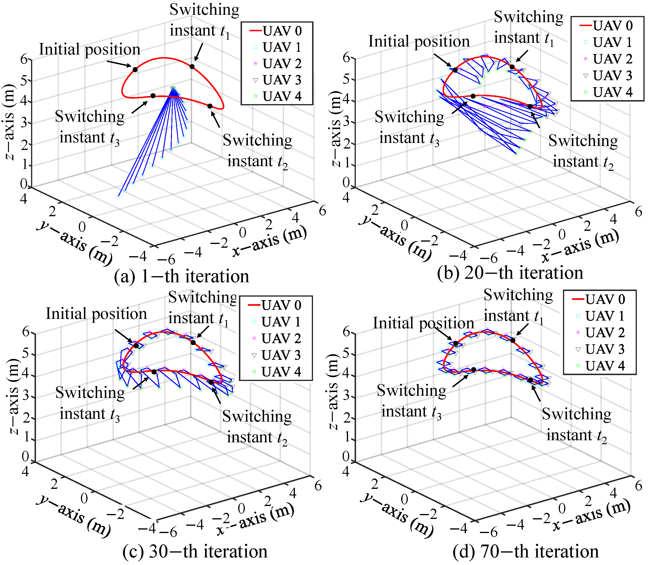
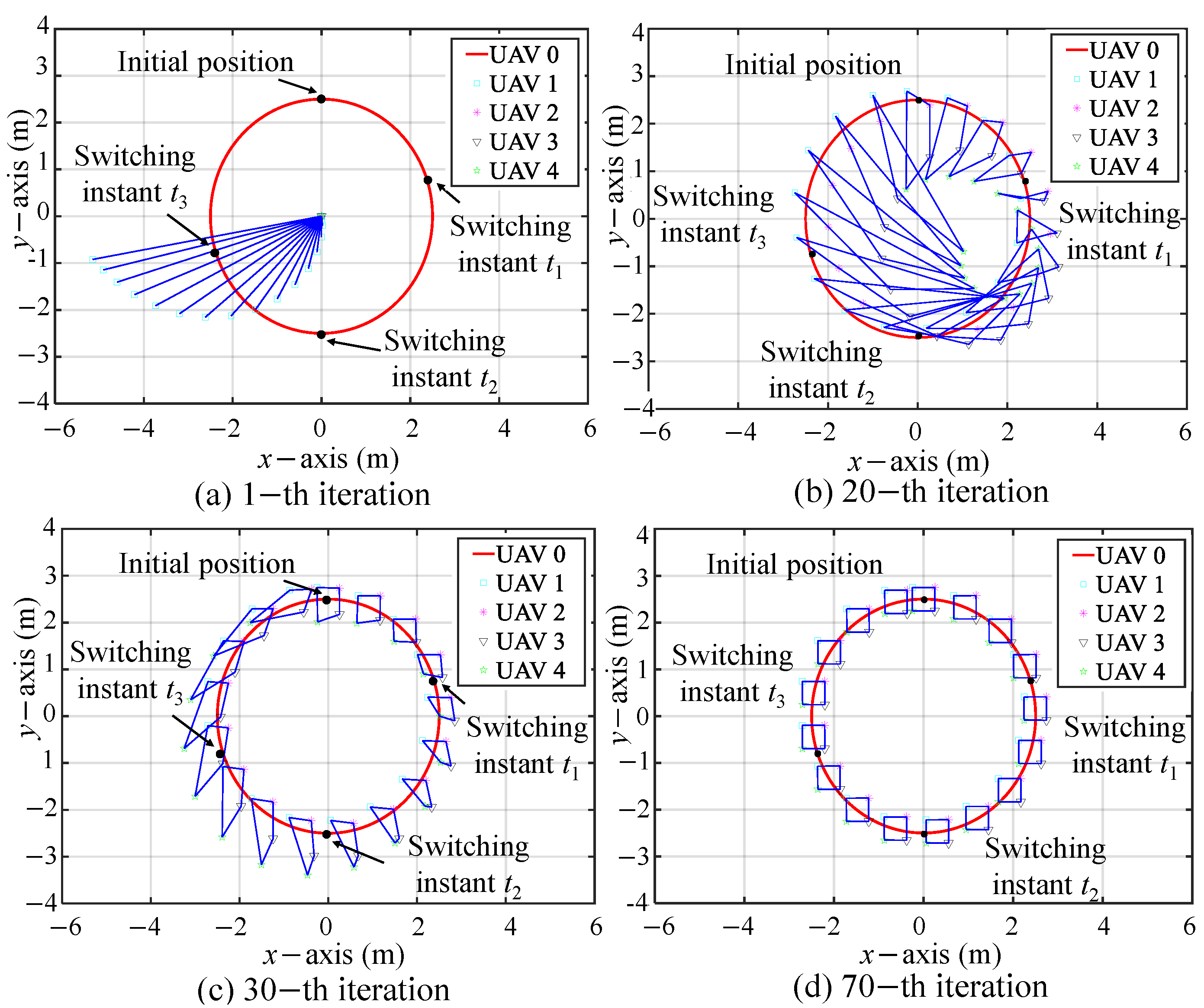
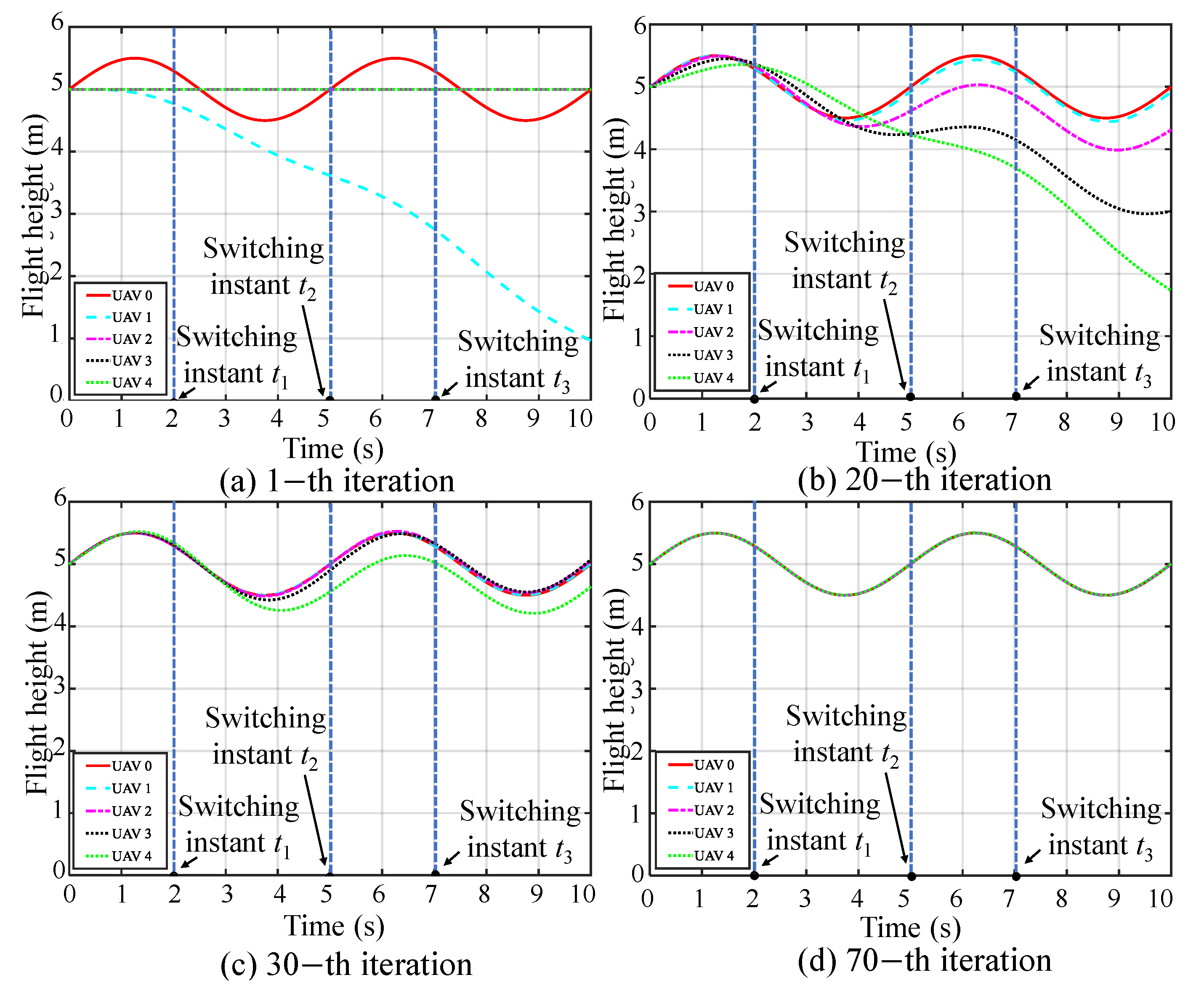
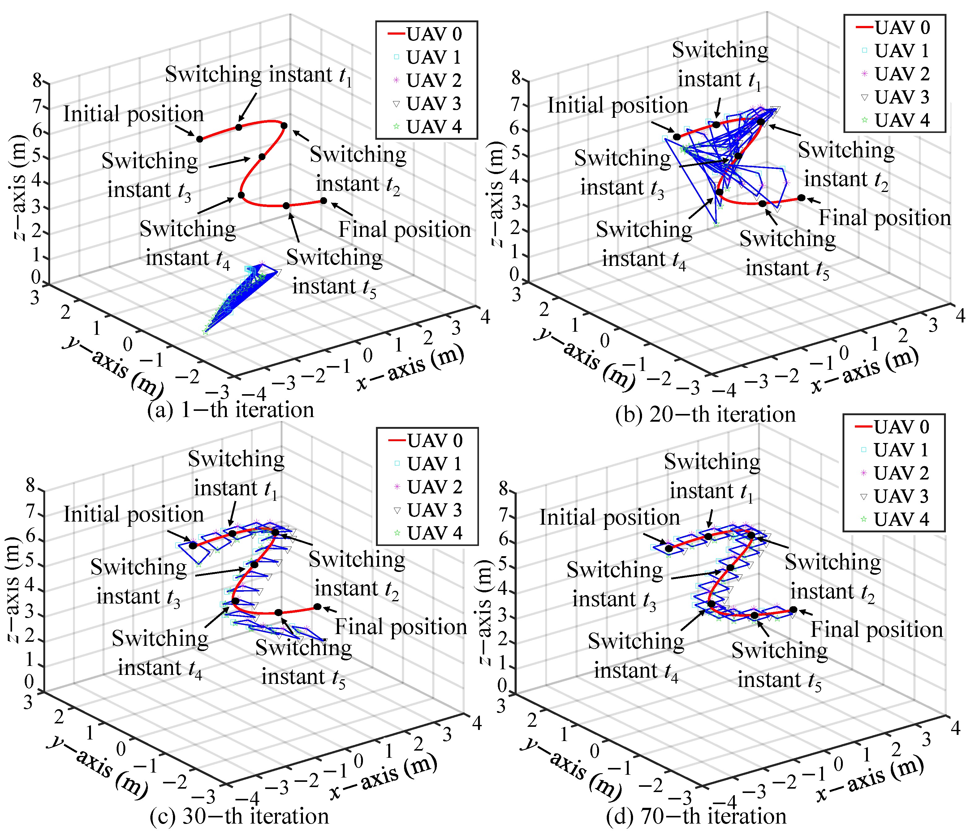
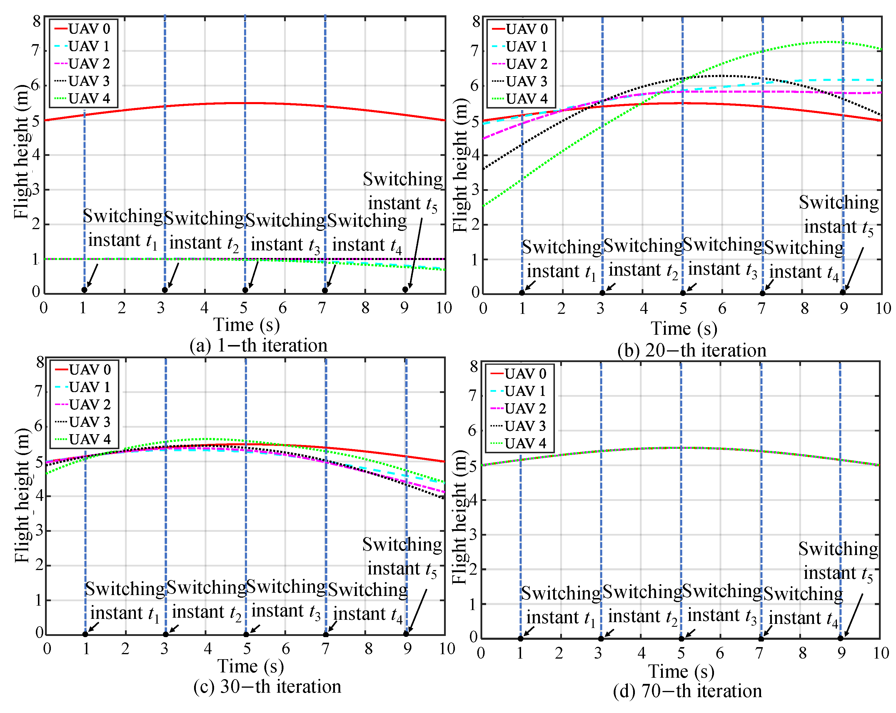
5.1. Simulation I: Formation Tracking with Switching Operating Modes

This subsection gives a simulation experiment that considers a multi-UAV system with four quadrotor UAVs, in which each quadrotor UAV has two operating modes: the on-load and no-load operating modes. The dynamic models of the multi-quadrotor UAV system with two operating modes are given as follows:

(1) The quadrotor UAV under the no-load operating mode [41]:

$$\begin{array}{c}\hfill \left\{\begin{array}{cc}& \dot{\xi }=v\hfill \\ & \dot{\varpi }=R\alpha \hfill \\ & m\dot{v}=m{A}_{1}v+F\hfill \\ & J\dot{\alpha }=\alpha \times \left(J\alpha \right)+M\hfill \end{array}\right.\end{array}$$

(61)

where $m=8$ kg is the mass of each UAV, $\xi ={[p_x,p_y,p_x]}^{\mathrm{T}}$ is the position vector, $v={[v_x,v_y,v_z]}^{\mathrm{T}}$ is the linear velocity vector, $\varpi ={[\varphi ,\theta ,\phi ]}^{\mathrm{T}}$ is the three Euler angles, i.e., roll angle $\varphi$, pitch angle $\theta$, and yaw angle $\phi$. $\alpha ={[{\alpha }_x,{\alpha }_y,{\alpha }_z]}^{\mathrm{T}}$ is the angular velocity vector, $F={[F_x,F_y,F_z]}^{\mathrm{T}}$ is the projection component of thrust in the $xyz$—directions on the body frame, and $M={[u_{\varphi },u_{\theta },u_{\phi }]}^{\mathrm{T}}$ is the input torque vector. For simplicity, we omit t and h in (61) (the same as below).

$$\begin{array}{cc}& R=\left[\begin{array}{ccc}1& tan\theta sin\varphi & tan\theta cos\varphi \\ 0& cos\varphi & -sin\varphi \\ 0& sin\varphi /cos\theta & cos\varphi /cos\theta \end{array}\right],A_1=\left[\begin{array}{ccc}0& {\alpha }_z& -{\alpha }_y\\ -{\alpha }_z& 0& {\alpha }_x\\ {\alpha }_y& -{\alpha }_x& 0\end{array}\right].J=\left[\begin{array}{ccc}{J}_x& J_{xy}& J_{xz}\\ J_{xy}& J_y& J_{yz}\\ J_{xz}& J_{yz}& J_z\end{array}\right].\hfill \end{array}$$

Here, $J_x=4$, $J_y=4$, $J_z=8.8$, $J_{xy}=0.031$, $J_{xz}=0.011$, and $J_{yz}=0.023$. Here, without a loss of generality, we assume that the quadrotor UAVs are always flying with small attitude angles, i.e., $R\approx I_3$.

According to the dynamic model (1), the system vectors and matrices are

$$\begin{array}{cc}\hfill & x_1^{\left(j\right)}(t,h)={[{\xi }^{\mathrm{T}},{\varpi }^{\mathrm{T}}]}^{\mathrm{T}},x_2^{\left(j\right)}(t,h)={[v^{\mathrm{T}},{\alpha }^{\mathrm{T}}]}^{\mathrm{T}},y^{\left(j\right)}(t,h)={[{\xi }^{\mathrm{T}},{\varpi }^{\mathrm{T}}]}^{\mathrm{T}},u^j(t,h)={[F^{\mathrm{T}},M^{\mathrm{T}}]}^{\mathrm{T}},\hfill \\ \hfill & f_1\left(x(t,h)\right)={[{\left(A_{1}v\right)}^{\mathrm{T}},J^{-1}{(\alpha \times \left(J\alpha \right))}^{\mathrm{T}}]}^{\mathrm{T}},C_1=I_6,{\omega }_1^{\left(j\right)}(t,h)=0.2sin\left(0.1h\right)sin\left(2\pi t\right){\mathbf{1}}_6,\hfill \\ \hfill & B_1=\mathrm{diag}(I_3/m,J^{-1}).\hfill \end{array}$$

(2) The quadrotor UAV under the on-load operating mode [41]:

For each quadrotor UAV, the load is suspended by a massless cable attached at the center of the quadrotor UAV. Thus, the position vector of the load in the body frame of the UAV is $r=[0,0,-(l+z_h)]$, where $l=0.4$ m is the cable length, and $z_h=0.1$ m is the distance between the suspension point and the center of mass of the quadrotor UAV. The mass of each load is $m_0=0.1$ kg. Hence, the dynamic mode of the quadrotor UAV in the on-load operating mode is

$$\begin{array}{c}\hfill \left\{\begin{array}{cc}& \dot{\xi }=v\hfill \\ & \dot{\varpi }=R\alpha \hfill \\ & (m+m_0)\dot{v}=m{A}_{1}v+F+F_p\hfill \\ & J_p\dot{\alpha }=A_2\alpha +M+M_p\hfill \end{array}\right.\end{array}$$

(62)

where additional force $F_p$ and moment $M_p$ are related to the load, and the other parameters are

$$\begin{array}{cc}& J_p=\left[\begin{array}{ccc}{J}_x+m_0{z}_h(z_h+l)& J_{xy}& J_{xz}\\ J_{xy}& J_y+m_0{z}_h(z_h+l)& J_{yz}\\ J_{xz}& J_{yz}& J_z\end{array}\right],A_2=\left[\begin{array}{ccc}{ϵ}_{11}& {ϵ}_{12}& {ϵ}_{13}\\ {ϵ}_{21}& {ϵ}_{22}& {ϵ}_{23}\\ {ϵ}_{31}& {ϵ}_{32}& {ϵ}_{33}\end{array}\right],\hfill \\ & {ϵ}_{11}=-J_{xz}{\alpha }_y+J_{xy}{\alpha }_z,{ϵ}_{12}=m_0{z}_h{\alpha }_z(z_h+l)-J_{yz}{\alpha }_y-(J_z-J_y){\alpha }_z,{ϵ}_{13}=J_{yz}{\alpha }_z,\hfill \\ & {ϵ}_{21}=-{\alpha }_z{m}_0{z}_h(z_h+l)+J_{xz}{\alpha }_x-(J_x-J_z){\alpha }_z,{ϵ}_{22}=J_{yz}{\alpha }_x-J_{xy}{\alpha }_z,{ϵ}_{23}=-J_{xz}{\alpha }_z,\hfill \\ & {ϵ}_{31}=-J_{xy}{\alpha }_x+(J_x-J_y){\alpha }_y,{ϵ}_{32}=J_{xy}{\alpha }_y+\left(J_{xz}\right){\alpha }_z,{ϵ}_{33}=-J_{yz}{\alpha }_x,\hfill \\ & M_p={(0,0,-z_h)}^{\mathrm{T}}\times g_p,F_p=-m_0(\alpha \times (\alpha \times r))+g_p,g_p={[0,0,-m_{0}g]}^{\mathrm{T}}.\hfill \end{array}$$

According to the dynamic model (1), the system vectors and matrices are

$$\begin{array}{cc}\hfill & f_2\left(x(t,h)\right)=J_2^{-1}{[{(m{A}_{1}v+F_p)}^{\mathrm{T}},{(A_2\alpha +M_p)}^{\mathrm{T}}]}^{\mathrm{T}},B_2=J_2^{-1},C_2=I_6,\hfill \\ \hfill & {\omega }_2^{\left(j\right)}(t,h)=0.2sin\left(0.01h\right)cos\left(2\pi t\right){\mathbf{1}}_6.\hfill \end{array}$$

where

$$\begin{array}{c}\hfill \begin{array}{cc}& J_2=\left[\begin{array}{cc}(m+m_0)I_3& J_{22}\\ J_{23}& J_p\end{array}\right],J_{22}=\left[\begin{array}{ccc}0& -m_0{z}_h& 0\\ m_0{z}_h& 0& 0\\ 0& 0& 0\end{array}\right],J_{23}=\left[\begin{array}{ccc}0& -m_0(z_h+l)& 0\\ m_0(z_h+l)& 0& 0\\ 0& 0& 0\end{array}\right].\hfill \end{array}\end{array}$$

The operating mode switching law $s\left(t\right)$ is defined in Figure 3. If $s\left(t\right)=1$, then the multi-quadrotor system is working under the on-load operating mode; if $s\left(t\right)=2$, then the multi-quadrotor system is working under the on-load operating mode. The total runtime is $T=1$ s and the max iteration number is $h_{max}=100$. The initial states are $x_1^{\left(j\right)}(0,0)={[0,0,5,0,0,0]}^{\mathrm{T}}$ and $x_2^{\left(j\right)}(0,0)={\mathbf{0}}_n$. The initial iterative input is $u^{\left(j\right)}(t,0)={\mathbf{0}}_p$, ($j=1,2,3,4$). The trajectory of the virtual leader quadrotor UAV is $y_d\left(t\right)={[2.5sin\left(0.2\pi t\right),2.5cos\left(0.2\pi t\right),5+0.5sin\left(0.4\pi t\right),0.2cos\left(0.2\pi t\right),0,0]}^{\mathrm{T}}$. The desired formation deviations between the four quadrotor UAVs and the leader are $d_1=[-0.25,0.25,0,0,0,0]$, $d_2=[0.25,0.25,0,0,0,0]$, $d_3=[-0.25,-0.25,0,0,0,0]$ and $d_4=[0.25,-0.25,0,0,0,0]$, respectively. The initial iterative disturbance is ${\widehat{\omega }}_{s\left(t\right)}^{\left(j\right)}(t,0)={\mathbf{0}}_n$, ($j=1,2,3,4$). The communication topology of the four quadrotors is shown in Figure 4, and we calculate that $\Psi =\left[\begin{array}{cccc}1& 0& 0& 0\\ -1& 1& 0& 0\\ 0& -1& 1& 0\\ 0& 0& -1& 1\end{array}\right]\otimes I_4$. For the ILO (6), we choose the observer gain matrices as $K_1=K_2=0.5I_{24}$ and $L_1=L_2=0.5I_{24}$. For the ILC algorithm (11)–(14), we choose the control gain matrices as $K_1^x=K_2^x=0.5I_{24}$, $K_1^{\omega }=K_2^{\omega }=0.5I_{24}$, and ${\Lambda }_1={\Lambda }_2=0.5I_{24}$. ${\Gamma }_1=2.1I_{24}$ and ${\Gamma }_2=2.4I_{24}$. Hence, with the determined gain matrices and a fixed communication topology, the convergence conditions (15) and (33) are verified, i.e.,

$$\begin{array}{cc}& \mathrm{If}s\left(t\right)=1,\mathrm{then}\left\{\begin{array}{c}\parallel I_{24}-L_1{\tilde{C}}_1\parallel =0.5000<1\hfill \\ & \parallel I_{24}-{\tilde{C}}_1{\tilde{B}}_1{\Gamma }_1\Psi \parallel =0.9612<1\hfill \end{array}\right.\hfill \\ & \mathrm{If}s\left(t\right)=2,\mathrm{then}\left\{\begin{array}{cc}& \parallel I_{24}-L_2{\tilde{C}}_2\parallel =0.5000<1\hfill \\ & \parallel I_{24}-{\tilde{C}}_2{\tilde{B}}_2{\Gamma }_2\Psi \parallel =0.9570<1\hfill \end{array}\right.\hfill \end{array}$$

The simulation results are shown in Figure 5, Figure 6, Figure 7, Figure 8, Figure 9 and Figure 10.

The formation trajectories of the quadrotor UAVs at the $xyz$ coordinate and in the $xoy$ plane at different iterations are shown in Figure 5 and Figure 6, respectively. It can be easily seen from Figure 5 and Figure 6 that the four quadrotor UAVs can form a square formation well and track the leader quadrotor UAV over the all-time steps after 70 iterations, although the dynamic models of the quadrotor UAVs are varied at different time intervals. Figure 7 and Figure 8 indicate that all the follower quadrotor UAVs keep the same flight height and yaw angle as the leader quadrotor UAV. The average and maximal formation tracking error of the four quadrotor UAVs along the iteration axis are shown in Figure 9a,b, respectively, where $T_{sam}=1000$ is the total number of data samples. This demonstrates the convergence of the formation tracking errors in the iteration domain, and this implies that the formation objective (4) is successfully achieved. The maximal state observer errors $e^{x_1}(t,h)$ and $e^{x_2}(t,h)$ are shown in Figure 10a, and the maximal disturbance estimation error $e^{\omega }(t,h)$ is shown in Figure 10b. From these figures, we can see that the state and disturbance estimation errors converge to a small range around zero with the increasing iteration number. Hence, Theorem 1 and 2 under the switching operating modes are verified.

5.2. Simulation II: Formation Tracking with Switching Topologies

In this subsection, a simulation of a multi-quadrotor UAV system under the on-load operating mode (62) with switching topologies is conducted. According to the switching law in Figure 11 and the possible switching communication topologies are illustrated in Figure 12, we denote that if $s\left(t\right)=1$, then the sub-topology ${\overline{\mathcal{G}}}_1$ is active; if $s\left(t\right)=2$, then the sub-topology ${\overline{\mathcal{G}}}_2$ is active. The initial states are $x_1^{\left(1\right)}(0,0)={[-0.25,0.25,1,0,0,0]}^{\mathrm{T}}$, $x_1^{\left(2\right)}(0,0)={[0.25,0.25,1,0,0,0]}^{\mathrm{T}}$, $x_1^{\left(3\right)}(0,0)={[0.25,-0.25,1,0,0,0]}^{\mathrm{T}}$, $x_1^{\left(4\right)}(0,0)={[-0.25,-0.25,1,0,0,0]}^{\mathrm{T}}$, and $x_2^{\left(j\right)}(0,0)={\mathbf{0}}_n$, ($j=1,2,3,4$). The trajectory of the virtual leader quadrotor UAV is $y_d\left(t\right)=[2sin\left(0.2\pi t\right),2cos\left(0.1\pi t\right),5+0.5sin\left(0.1\pi t\right),$${0.1cos\left(0.2\pi t\right),0,0]}^{\mathrm{T}}$, and the other parameters are set to be the same as in Simulation I. According to Figure 12, we can calculate that ${\Psi }_1=\left[\begin{array}{cccc}1& 0& 0& 0\\ -1& 1& 0& 0\\ 0& -1& 1& 0\\ 0& 0& -1& 1\end{array}\right]\otimes I_4$, and ${\Psi }_2=\left[\begin{array}{cccc}1& 0& 0& -1\\ -1& 1& 0& 0\\ 0& -1& 1& 0\\ 0& 0& 0& 1\end{array}\right]\otimes I_4$.

Similar to Simulation I, we determine the observer and control gain matrices as $K_1=K_2=0.2I_{24}$, $L_1=L_2=0.9I_{24}$, $K_1^x=K_2^x=0.5I_{24}$, $K_1^{\omega }=K_2^{\omega }=0.5I_{24}$, and ${\Lambda }_1={\Lambda }_2=0.5I_{24}$. ${\Gamma }_1=2.7I_{24}$ and ${\Gamma }_2=2.5I_{24}$. Hence, with a fixed on-load operating mode (62), the convergence condition (15) and (33) are verified, i.e.,

$$\begin{array}{cc}& \mathrm{If}s\left(t\right)=1,\mathrm{then}\left\{\begin{array}{cc}& \parallel I_{24}-L_1{\tilde{C}}_2\parallel =0.9000<1\hfill \\ & \parallel I_{24}-{\tilde{C}}_2{\tilde{B}}_2{\Gamma }_1{\Psi }_1\parallel =0.9508<1\hfill \end{array}\right.\hfill \\ & \mathrm{If}s\left(t\right)=2,\mathrm{then}\left\{\begin{array}{cc}& \parallel I_{24}-L_2{\tilde{C}}_2\parallel =0.9000<1\hfill \\ & \parallel I_{24}-{\tilde{C}}_2{\tilde{B}}_2{\Gamma }_2{\Psi }_2\parallel =0.9557<1\hfill \end{array}\right.\hfill \end{array}$$

The simulation results are shown in Figure 13, Figure 14, Figure 15, Figure 16, Figure 17 and Figure 18. The formation trajectories are shown in Figure 13 and Figure 14. After 70 iterations, a square formation of four quadrotor UAVs can be maintained under switching communication topologies. Meanwhile, Figure 15 and Figure 16 show that all the quadrotor UAVs have the same flight height and yaw angle as the leader UAV. Figure 17 shows the formation tracking error along the iteration axis. We can see that the formation tracking errors are convergent in the iteration domain. The maximal state observer errors $e^{x_1}(t,h)$ and $e^{x_2}(t,h)$ and the maximal disturbance estimation error $e^{\omega }(t,h)$ are shown in Figure 18a,b. As a result, Theorems 1 and 2 under switching topologies are also verified.

5.3. Simulation III: Compared to the PID Controller

In this subsection, we conduct a comparison simulation experiment with a PID controller that is described as

$$\begin{array}{cc}\hfill u_{PID}\left(t\right)=& K_P\Psi (e\left(t\right)+\dot{e}\left(t\right))+K_D\Psi (\dot{e}\left(t\right)+\ddot{e}\left(t\right))+K_I{\int }_0^t\Psi (e\left(\tau \right)+\dot{e}\left(\tau \right))\mathrm{d}\tau \hfill \end{array}$$

(63)

where $K_P=25I_{24}$, $K_D=6I_{24}$, and $K_I=20I_{24}$ are the control gains. The stability of the PID controller (63) for a second-order dynamic system is analyzed in Reference [42]. The multi-quadrotor UAV system is considered to be same as that in Simulation I. The comparison experiment results are shown in Figure 19 and Figure 20. For the simulation of the ILC controller, the results are obtained after 70 iterations. Figure 19 illustrates the formation tracking trajectories with the ILC strategy and PID controller, respectively. Compared to the tracking trajectory with the PID controller, perfect formation tracking during the entire working time interval can be achieved with two distinct operating modes. Meanwhile, Figure 20 gives the formation tracking errors with the ILC strategy and PID controller, respectively. Furthermore, we summarize the average formation tracking errors of the four quadrotor UAVs with the proposed formation strategy and PID controller in

Table 1. Comparative results of the average formation tracking errors of four quadrotor UAVs with the proposed hybrid formation strategy and PID controller.

Controller	${\mathit{p}}_{\mathit{x}}$ (m)	${\mathit{p}}_{\mathit{y}}$ (m)	${\mathit{p}}_{\mathit{z}}$ (m)	$\mathit{\phi }$ (rad)
Controller (12)	0.0047 m	0.0110 m	0.0018 m	0.0024 rad
PID controller	0.0478 m	0.2223 m	0.0790 m	0.2190 rad

, which also demonstrates the superiority of the proposed formation strategy in this paper.

Consequently, the simulation results indicate that the four quadrotor UAVs can successfully track the leader quadrotor UAVs while maintaining a desired square formation. This further demonstrates the effectiveness of the proposed hybrid iterative learning strategy for the multi-UAV system by considering the multi-operating modes, switching communication topologies, and unknown external disturbances. Additionally, compared to the PID controller, the proposed hybrid iterative learning formation can ensure perfect formation tracking over the entire working time interval and has a higher precision tracking performance. Meanwhile, the calculation time of the proposed formation controller is about 0.009s in an iteration, and this is far less than the actual task cycle time, $T=10$ s, set in the simulations. Thus, the proposed method displays a good real-time performance.

6. Conclusions

In this paper, we propose a hybrid iterative learning formation strategy for the formation control problem of multi-UAV systems with multi-operating modes, switching communication topologies, and unknown external disturbances. Considering the fact that an accurate dynamic model of a multi-UAV system is hard to obtain, the proposed iterative learning formation controller uses the stored historical data to update the control input along the iterative axis without relying on the model’s knowledge of multi-UAV systems. Meanwhile, detailed theoretical results are given to guarantee the convergence of the estimation errors and formation tracking errors under multi-operating modes, switching communication topologies, and unknown external disturbances. Two sufficient convergence theorems can determine the appropriate observer and control gain matrices. At last, three formation flying simulations using four quadrotor UAVs under two different operating modes, switching topologies, and external disturbances demonstrate the effectiveness and superiority of the proposed formation strategy.

The limitation of the proposed method is that identical task trial lengths are required for different iterations. That is to say, the given goal task of multi-UAV systems with the proposed iterative learning strategy must be repeatable and have the same time cycle in different iterations. This repeatable characteristic ensures that the proposed iterative learning strategy has the learning ability to continuously improve the control performance over multiple iterations. However, this also causes some limitations of the proposed iterative learning strategy when extending to the non-strictly repeatable goal tasks. Thus, some researchers have attempted to solve the problem of varying trial lengths of iterative learning formation control [43,44], but the problem of the iterative learning formation control of multi-UAV systems with varying trial lengths is still open for discussion. Therefore, our future work will focus on the coordination control of multi-UAV systems with non-strictly repeatable application scenarios and varying trial lengths. In addition, the implementation of the proposed approach in practical UAVs may be limited by the computational resources of the practical control devices if the total number of UAVs is too large. Thus, the design of practical control units for UAVs should be a trade-off between the computing resources and the number of practical UAVs.

References

1. Li, Q.; Hua, Y.; Dong, X.; Yu, J.; Ren, Z. Time-varying formation tracking control for unmanned aerial vehicles with the leader’s unknown input and obstacle avoidance: Theories and applications. Electronics 2022, 11, 2334. [Google Scholar] [CrossRef]
2. Du, B.; Li, S. A new multi-satellite autonomous mission allocation and planning method. Acta Astronaut. 2019, 163, 287–298. [Google Scholar] [CrossRef]
3. Xiao, P.; Li, N.; Xie, F.; Ni, H.; Zhang, M.; Wang, B. Clustering-based multi-region coverage-path planning of heterogeneous UAVs. Drones 2023, 7, 664. [Google Scholar] [CrossRef]
4. Zhao, F.; Hua, Y.; Zheng, H.; Yu, J.; Dong, X.; Li, Q.; Ren, Z. Cooperative target pursuit by multiple fixed-wing UAVs based on deep reinforcement learning and artificial potential field. In Proceedings of the 2023 42nd Chinese Control Conference (CCC), Tianjin, China, 24–26 July 2023; pp. 5693–5698. [Google Scholar]
5. Moein, D.; Kabganian, M.; Azimi, A. Robust adaptive control for formation-based cooperative transportation of a payload by multi quadrotors. Eur. J. Control 2023, 69, 100763. [Google Scholar]
6. Zhang, J.; Yan, J.; Zhang, P. Multi-UAV formation control based on a novel back-stepping approach. IEEE Trans. Veh. Technol. 2020, 69, 2437–2448. [Google Scholar] [CrossRef]
7. Muslimov, T.Z.; Munasypov, R.A. Adaptive decentralized flocking control of multi-UAV circular formations based on vector fields and backstepping. ISA Trans. 2020, 107, 143–159. [Google Scholar] [CrossRef]
8. Balch, T.; Arkin, R.C. Behavior-based formation control for multirobot teams. IEEE Trans. Robot. Autom. 1998, 14, 926–939. [Google Scholar] [CrossRef]
9. Pan, Z.; Zhang, C.; Xia, Y.; Xiong, H.; Shao, X. An improved artificial potential field method for path planning and formation control of the multi-UAV systems. IEEE Trans. Circuits Syst. II Express Briefs 2021, 69, 1129–1133. [Google Scholar] [CrossRef]
10. Hua, Y.; Dong, X.; Hu, G.; Li, Q.; Ren, Z. Distributed time-varying output formation tracking for heterogeneous linear multiagent systems with a nonautonomous leader of unknown input. IEEE Trans. Autom. Control 2019, 64, 4292–4299. [Google Scholar] [CrossRef]
11. Yu, Y.; Guo, J.; Ahn, C.K.; Xiang, Z. Neural adaptive distributed formation control of nonlinear multi-UAVs with unmodeled dynamics. IEEE Trans. Neural Networks Learn. Syst. 2023, 34, 9555–9561. [Google Scholar] [CrossRef]
12. Cheng, C.; Zhang, H.; Sun, Y.; Tao, H.; Chen, Y. A cross-platform deep reinforcement learning model for autonomous navigation without global information in different scenes. Control Eng. Pract. 2024, 150, 105991. [Google Scholar] [CrossRef]
13. Li, R.; Wang, L.; Chen, Y.; Ma, P. Adaptive locomotion control of hexapod robot based on deep reinforcement learning and proprioception. In Proceedings of the 2023 6th International Conference on Robotics, Control and Automation Engineering, RCAE, Suzhou, China, 27–29 October 2023; pp. 39–43. [Google Scholar]
14. Han, D.; Jiang, H.; Wang, L.; Zhu, X.; Chen, Y.; Yu, Q. Collaborative task allocation and optimization solution for unmanned aerial vehicles in search and rescue. Drones 2024, 8, 138. [Google Scholar] [CrossRef]
15. Gong, B.; Jiang, L.; Ning, X.; Li, S. Study on mission planning algorithm for multi-target passive tracking based on satellite formation. Aerosp. Sci. Technol. 2023, 142, 108660. [Google Scholar] [CrossRef]
16. Wang, J.; Xin, M. Integrated optimal formation control of multiple unmanned aerial vehicles. IEEE Trans. Control Syst. Technol. 2013, 21, 1731–1744. [Google Scholar] [CrossRef]
17. Yan, D.; Zhang, W.; Chen, H. Design of a multi-constraint formation controller based on improved MPC and consensus for quadrotors. Aerospace 2022, 9, 94. [Google Scholar] [CrossRef]
18. Kuo, C.W.; Tsai, C.C.; Lee, C.T. Intelligent leader-following consensus formation control using recurrent neural networks for small-size unmanned helicopters. IEEE Trans. Syst. Man Cybern. Syst. 2019, 51, 1288–1301. [Google Scholar] [CrossRef]
19. Sun, R.; Zhou, Z.; Zhu, X. Finite-time terminal sliding mode attitude control for tailless full-wing configuration UAVs based on extended state observers and auxiliary compensators. ISA Trans. 2024, 144, 282–307. [Google Scholar] [CrossRef]
20. Ma, X.; Wang, G.; Liu, K. Design and optimization of a multimode amphibious robot with propeller-leg. IEEE Trans. Robot. 2022, 38, 3807–3820. [Google Scholar] [CrossRef]
21. Russo, S.; Harada, K.; Ranzani, T.; Manfredi, L.; Stefanini, C.; Menciassi, A.; Dario, P. Design of a robotic module for autonomous exploration and multimode locomotion. IEEE/ASME Trans. Mechatronics 2013, 18, 1757–1766. [Google Scholar] [CrossRef]
22. Xu, F.; Ma, K.; Gong, T.; Jiang, Z.; Hu, C. Design and testing of a magnetic soft crawling robot with multimodal locomotion driven by 3-D magnetic fields. IEEE Trans. Instrum. Meas. 2024, 73, 1–11. [Google Scholar] [CrossRef]
23. Xiong, X.; Ruan, X. Non-Smooth bifurcation analysis of multi-structure multi-operating-mode power electronics systems for applications with renewable energy sources. IEEE Trans. Circuits Syst. II Express Briefs 2019, 66, 487–491. [Google Scholar] [CrossRef]
24. Zou, Y.; Zhou, Z.; Dong, X.; Meng, Z. Distributed formation control for multiple vertical takeoff and landing UAVs with switching topologies. IEEE/ASME Trans. Mechatronics 2018, 23, 1750–1761. [Google Scholar] [CrossRef]
25. Wang, Z.; Liu, T.; Jiang, Z.P. Cooperative formation control under switching topology: An experimental case study in multirotors. IEEE Trans. Cybern. 2020, 51, 6141–6153. [Google Scholar] [CrossRef]
26. Zhou, Z.; Wang, H.; Wang, Y.; Xue, X.; Zhang, M. Distributed formation control for multiple quadrotor UAVs under Markovian switching topologies with partially unknown transition rates. J. Frankl. Inst. 2019, 356, 5706–5728. [Google Scholar] [CrossRef]
27. Xue, M.; Tang, Y.; Ren, W.; Qian, F. Practical output synchronization for asynchronously switched multi-agent systems with adaption to fast-switching perturbations. Automatica 2020, 116, 108917. [Google Scholar] [CrossRef]
28. Zhao, Z.; Wang, J.; Chen, Y.; Ju, S. Iterative learning-based formation control for multiple quadrotor unmanned aerial vehicles. Int. J. Adv. Robot. Syst. 2020, 17, 1729881420911520. [Google Scholar] [CrossRef]
29. Fu, X.; Peng, J. Iterative learning control for UAVs formation based on point-to-point trajectory update tracking. Math. Comput. Simul. 2023, 209, 1–15. [Google Scholar] [CrossRef]
30. Hock, A.; Schoellig, A.P. Distributed iterative learning control for multi-agent systems: Theoretic developments and application to formation flying. Auton. Robot. 2019, 43, 1989–2010. [Google Scholar] [CrossRef]
31. Han, Y.; Liang, Y.; Zhang, L.; Cai, B.; Li, Y.; Li, B. Bumpless transfer switched control of aircraft for heavy payload dropping missions. Aerosp. Sci. Technol. 2024, 148, 109067. [Google Scholar] [CrossRef]
32. Dong, X.; Zhou, Y.; Ren, Z.; Zhong, Y. Time-varying formation tracking for second-order multi-agent systems subjected to switching topologies with application to quadrotor formation flying. IEEE Trans. Ind. Electron. 2016, 64, 5014–5024. [Google Scholar] [CrossRef]
33. Wu, J.; Luo, C.; Luo, Y.; Li, K. Distributed UAV swarm formation and collision avoidance strategies over fixed and switching topologies. IEEE Trans. Cybern. 2022, 52, 10969–10979. [Google Scholar] [CrossRef]
34. Zhang, S.; Wang, L.; Wang, H.; Xue, B. Consensus control for heterogeneous multivehicle systems: An iterative learning approach. IEEE Trans. Neural Netw. Learn. Syst. 2021, 32, 5356–5368. [Google Scholar] [CrossRef]
35. Meng, D.; Zhang, J. Cooperative learning for switching networks with nonidentical nonlinear agents. IEEE Trans. Autom. Control 2021, 66, 6131–6138. [Google Scholar] [CrossRef]
36. Sun, M.; Wang, D. Sampled-data iterative learning control for nonlinear systems with arbitrary relative degree. Automatica 2001, 37, 283–289. [Google Scholar] [CrossRef]
37. Sun, M.; Huang, B. Iterative Learning Control; National Defence Industry Press: Beijing, China, 1999. [Google Scholar]
38. Meng, D.; Jia, Y.; Du, J.; Zhang, J. High-precision formation control of nonlinear multi-agent systems with switching topologies: A learning approach. Int. J. Robust Nonlinear Control 2015, 25, 1993–2018. [Google Scholar] [CrossRef]
39. Jeffreys, H.; Jeffreys, B.S. Methods of Mathematical Physics; Cambridge University Press: Cambridge, UK, 1999. [Google Scholar]
40. Shao, Z.; Xiang, Z. Design of an iterative learning control law for a class of switched repetitive systems. Circuits Syst. Signal Process. 2017, 36, 845–866. [Google Scholar] [CrossRef]
41. Shen, Z.; Tan, L.; Yu, S.; Song, Y. Fault-tolerant adaptive learning control for quadrotor UAVs with the time-varying CoG and full-state constraints. IEEE Trans. Neural Networks Learn. Syst. 2021, 32, 5610–5622. [Google Scholar] [CrossRef] [PubMed]
42. Zhao, C.; Guo, L. PID controller design for second order nonlinear uncertain systems. Sci. China-Inf. Sci. 2017, 60, 022201:1–022201:13. [Google Scholar] [CrossRef]
43. Shen, D.; Li, X. A survey on iterative learning control with randomly varying trial lengths: Model, synthesis, and convergence analysis. Annu. Rev. Control 2019, 48, 89–102. [Google Scholar] [CrossRef]
44. Zeng, C.; Shen, D.; Wang, J. Adaptive learning tracking for uncertain systems with partial structure information and varying trial lengths. J. Frankl. Inst. 2018, 355, 7027–7055. [Google Scholar] [CrossRef]
Figure 1. The control block diagram of the hybrid iterative learning formation strategy for the multi-UAV system (1) with multi-operating modes. The red arrows denote the switching behaviors.
Drones 08 00406 g001
Figure 2. The flowchart of the proposed method.
Drones 08 00406 g002
Figure 3. The switching law  s ( t )  of operating modes.
Drones 08 00406 g003
Figure 4. The communication topology  G ¯  and symbol “1” represents the connection weight.
Drones 08 00406 g004
Figure 5. The formation trajectory of the four quadrotor UAVs at  x y z  coordinates at 1−th, 20−th, 30−th, and 70−th iterations.
Drones 08 00406 g005
Figure 6. The formation trajectory of the four quadrotor UAVs on the  x o y  plane at 1−th, 20−th, 30−th, and 70−th iterations.
Drones 08 00406 g006
Figure 7. The flight heights of the four quadrotor UAVs at 1−th, 20−th, 30−th, and 70−th iterations.
Drones 08 00406 g007
Figure 8. The yaw angles of the four quadrotor UAVs at 1−th, 20−th, 30−th, and 70−th iterations.
Drones 08 00406 g008
Figure 9. The average and maximal formation tracking errors in the iteration domain.
Drones 08 00406 g009
Figure 10. The maximal state and disturbance estimation errors in the iteration domain.
Drones 08 00406 g010
Figure 11. The switching law  s ( t )  of communication topologies.
Drones 08 00406 g011
Figure 12. The possible switching communication topologies and symbol "1" represents the connection weight.
Drones 08 00406 g012
Figure 13. The formation trajectory of the four quadrotor UAVs at the  x y z  coordinate at 1−th, 20−th, 30−th, and 70−th iterations.
Drones 08 00406 g013
Figure 14. The formation trajectory of the four quadrotor UAVs in the  x o y  plane at 1−th, 20−th, 30−th, and 70−th iterations.
Drones 08 00406 g014
Figure 15. The flight heights of the four quadrotor UAVs at 1−th, 20−th, 30−th, and 70−th iterations.
Drones 08 00406 g015
Figure 16. The yaw angles of the four quadrotor UAVs at 1−th, 20−th, 30−th, and 70−th iterations.
Drones 08 00406 g016
Figure 17. The average and maximal formation tracking error in the iteration domain.
Drones 08 00406 g017
Figure 18. The maximal state and disturbance estimation errors in the iteration domain.
Drones 08 00406 g018
Figure 19. The formation trajectory of four quadrotor UAVs at the  x y z  coordinate with ILC controller and PID controller, respectively.
Drones 08 00406 g019
Figure 20. The formation tracking and estimation errors with ILC controller and PID controller, respectively.
Drones 08 00406 g020