
Collaborative Obstacle Detection for Dual USVs Using MGNN-DANet with Movable Virtual Nodes and Double Attention

Abstract
:1. Introduction
2. Related Work
2.1. Point Cloud Registration Methods
2.2. Template Matching Methods
2.3. Challenges of Template Matching Methods
2.4. Contributions
- (1)
- Advanced Collaborative Obstacle Detection Method
- (2)
- Innovative feature extraction with movable virtual nodes
- (3)
- Double attention-based feature matching
3. Methodology
3.1. Overview
3.2. Input Preprocessing
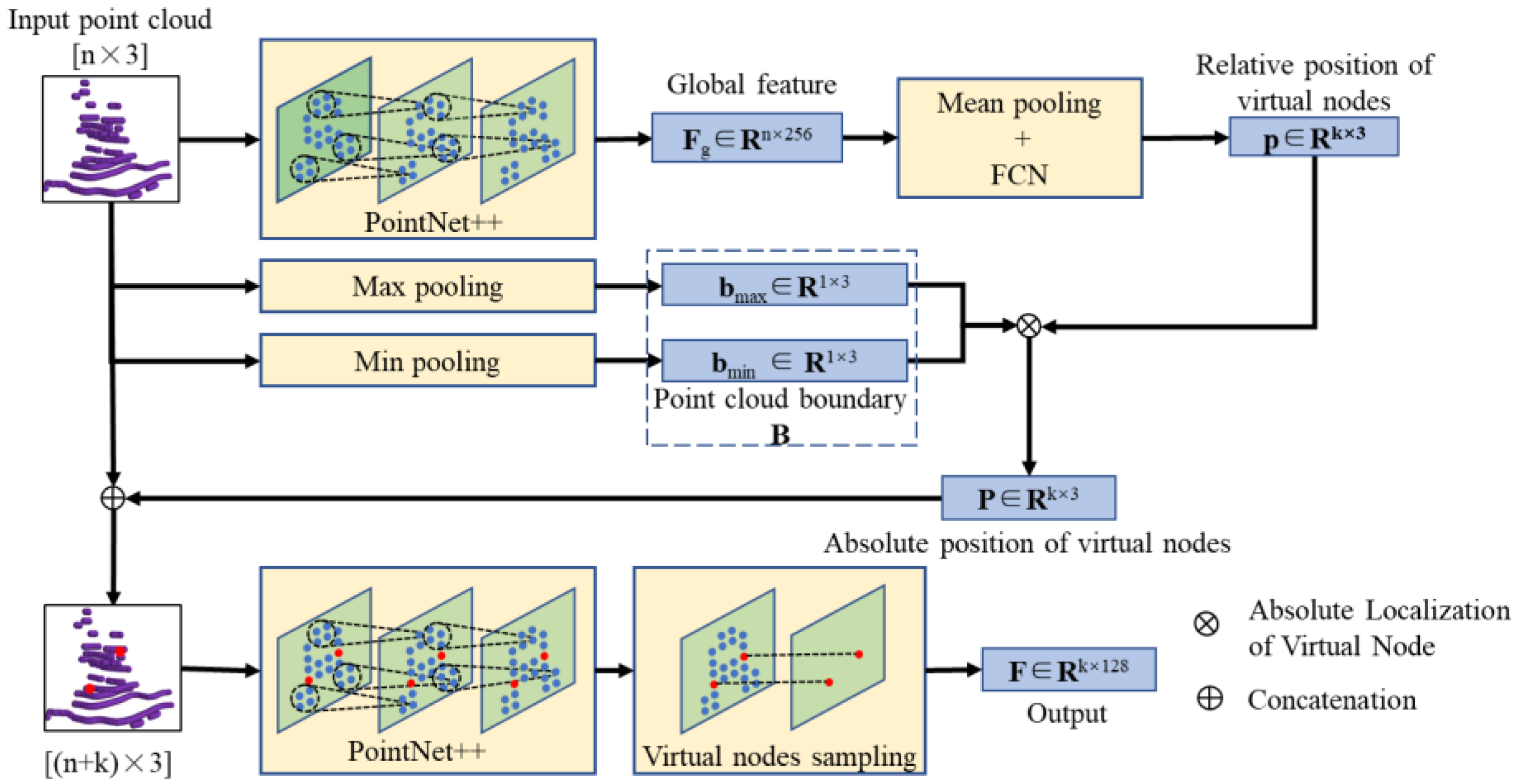
3.3. Feature Extraction
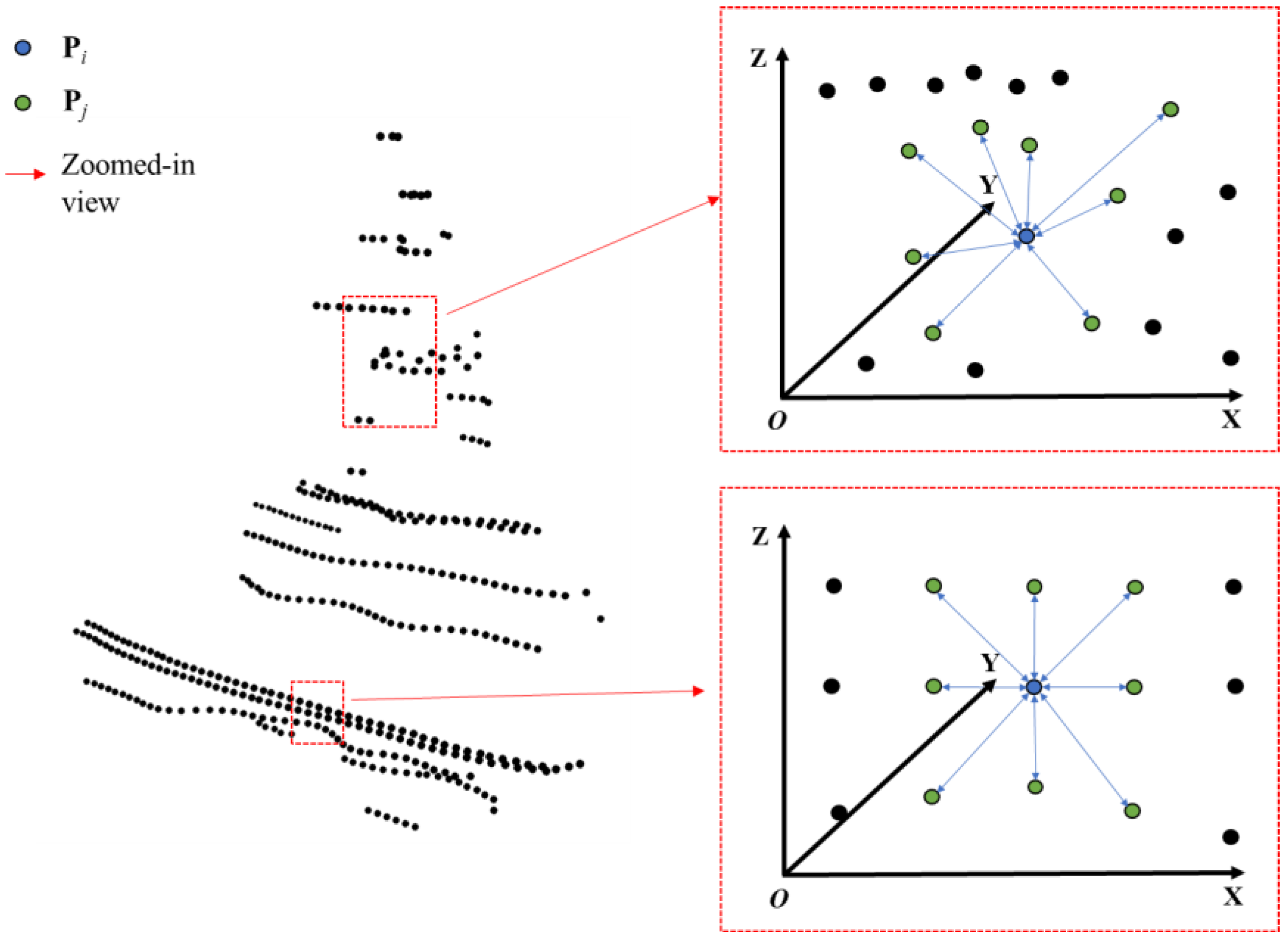
3.3.1. Generation of Movable Virtual Nodes
3.3.2. Positioning of Movable Virtual Nodes
3.3.3. Virtual Point Sampling
3.4. Feature Matching
3.4.1. Revisiting Attention Module
3.4.2. Feature Matching Model with Double Attention
3.5. Rotating and Clustering of Dual-View Point Cloud
4. Experiments
4.1. Validation of the Feature Extraction Model
4.1.1. Experimental Protocol
- (1)
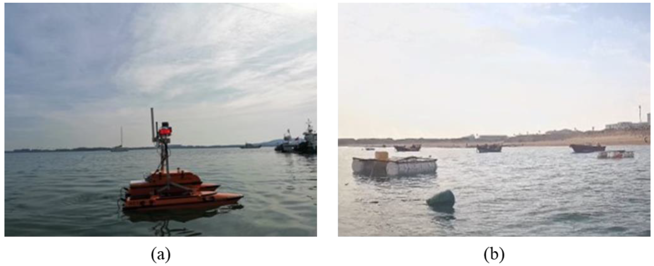
- Experimental data
- (2)
- Experimental setting
- (3)
- Evaluation metrics
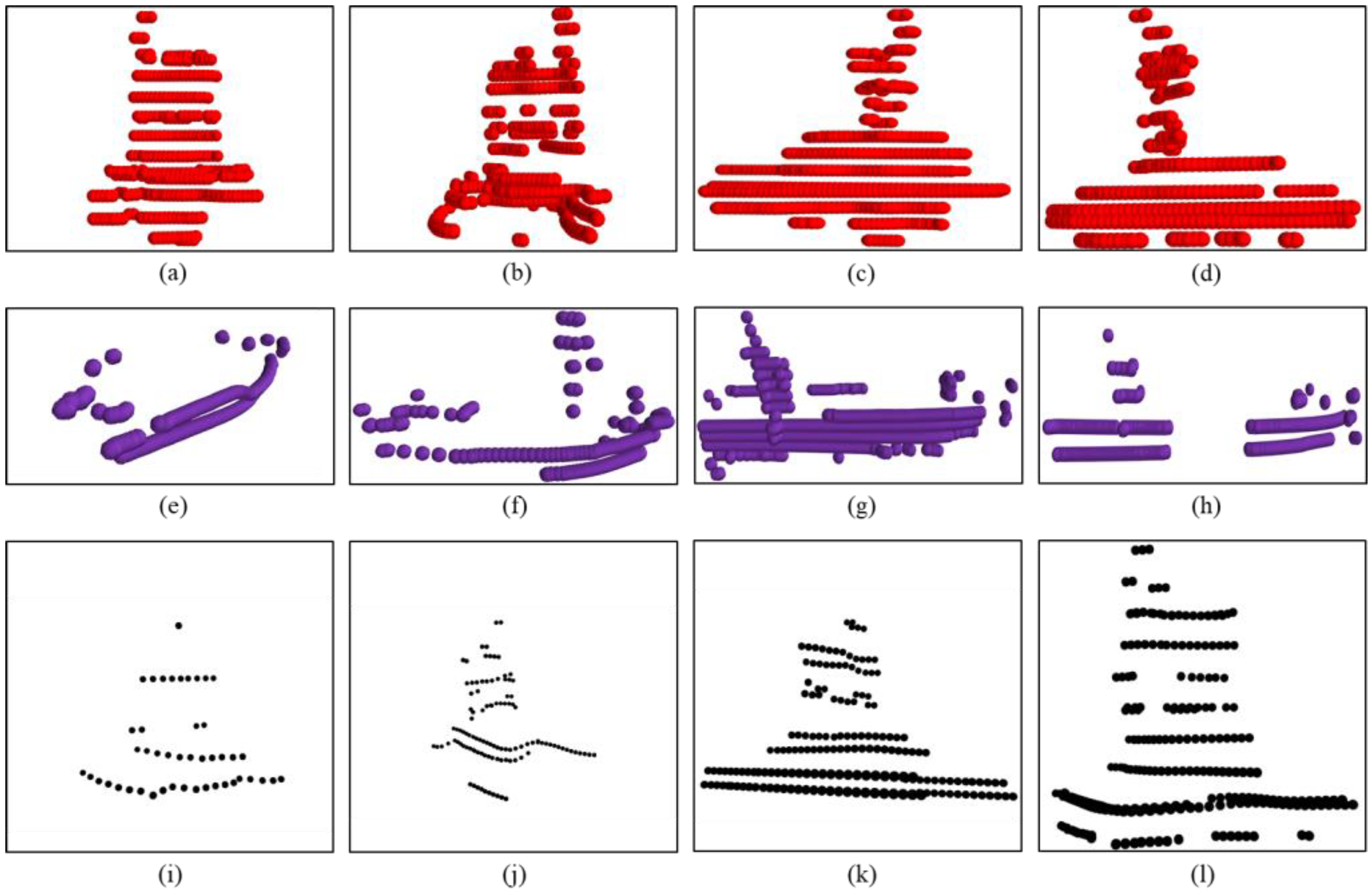
4.1.2. Experimental Results and Analysis
4.2. Validation of Feature Matching
4.2.1. Experimental Protocol
- (1)
- Experimental data
- (2)
- Experimental setting
- (3)
- Evaluation metrics
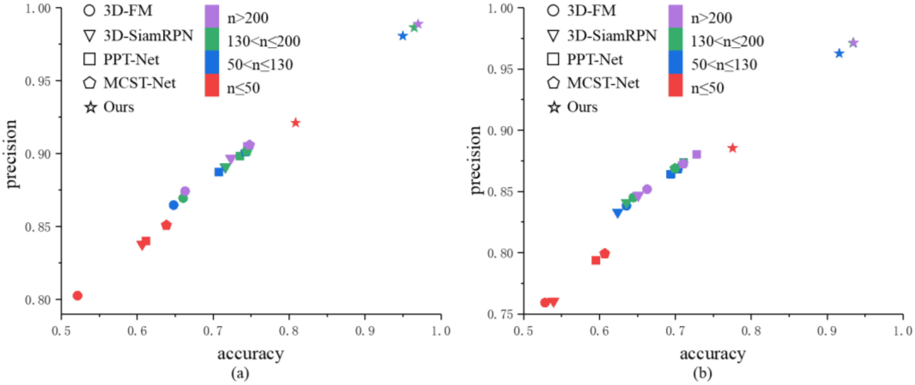
4.2.2. Experimental Results and Analysis
4.3. Validation of Obstacle Detection for Dual USVs
4.3.1. Experimental Protocol
- (1)
- Experimental data
- (2)
- Experimental setting
- (3)
- Evaluation metrics
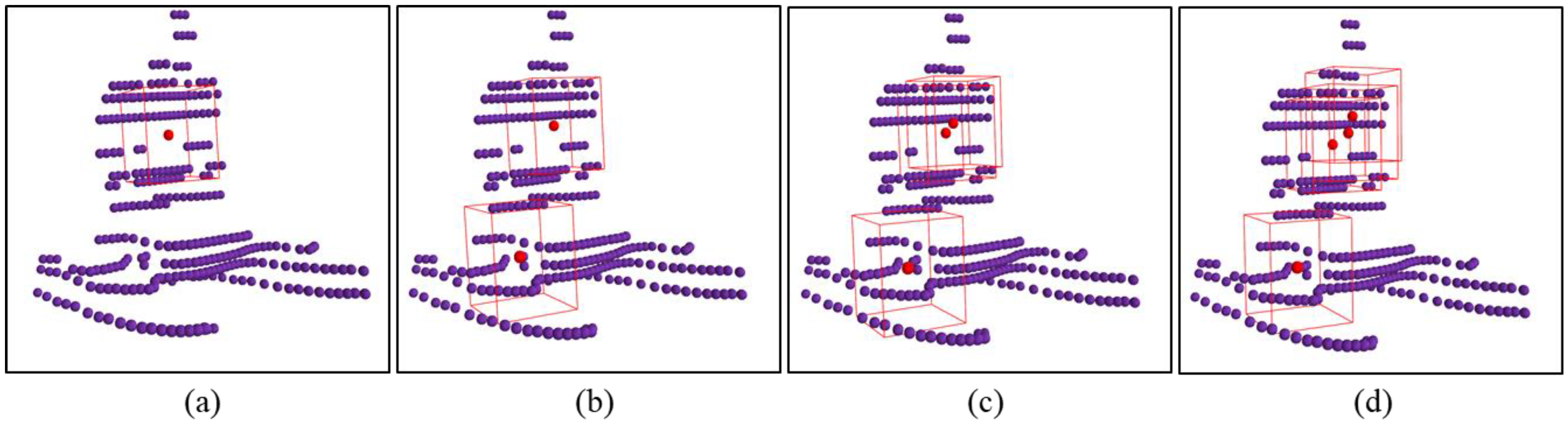
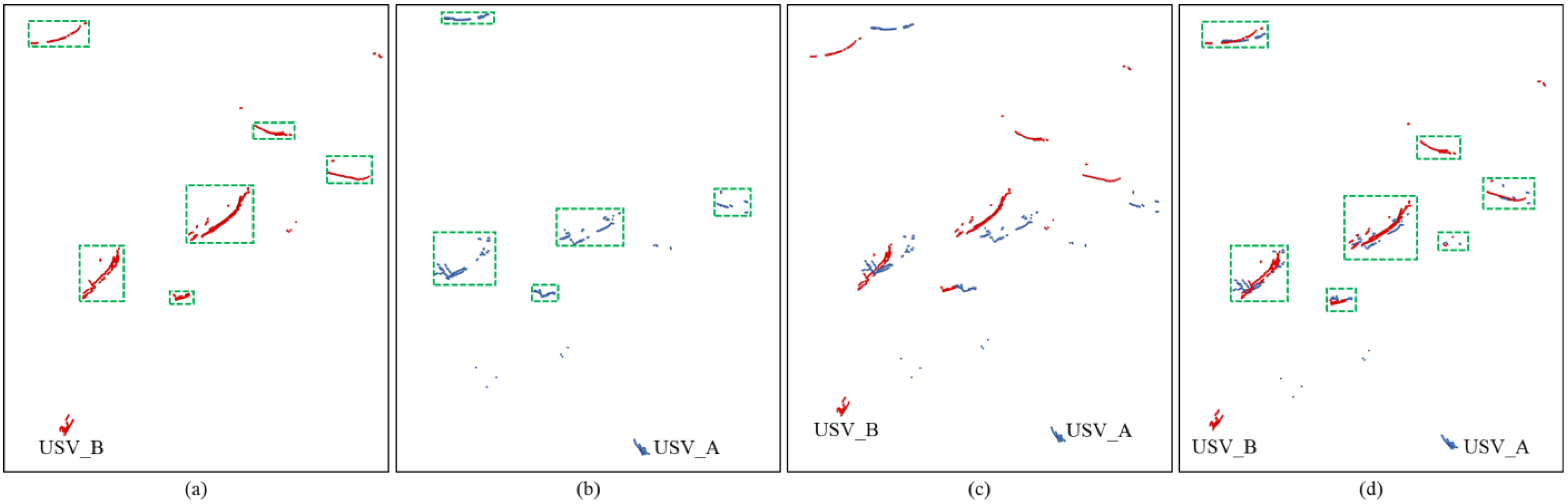
4.3.2. Qualitative Analysis
4.3.3. Quantitative Analysis
5. Conclusions
- Utilize high-precision map information to filter out point clouds from coastal areas.
- Implement an adaptive threshold mechanism that adjusts the sensitivity of template matching based on the distance to the coastline.
- Develop a point cloud registration method based on the overall coastline profile, aligning dual-view coastlines to correct point cloud positions.
- Integrate data from multiple sensors, such as LiDAR and cameras, to leverage their respective advantages and enhance the resilience of template matching against interference.
Author Contributions
Funding
Data Availability Statement
Conflicts of Interest
References
- Xiong, Y.; Zhu, H.; Pan, L.; Wang, J. Research on intelligent trajectory control method of water quality testing unmanned surface vessel. J. Mar. Sci. Eng. 2022, 10, 1252. [Google Scholar] [CrossRef]
- Ang, Y.; Ng, W.; Chong, Y.; Wan, J.; Chee, S.; Firth, L. An autonomous sailboat for environment monitoring. In Proceedings of the 2022 Thirteenth International Conference on Ubiquitous and Future Networks, Barcelona, Spain, 5–8 July 2022. [Google Scholar]
- Smith, T.; Mukhopadhyay, S.; Murphy, R.; Manzini, T.; Rodriguez, I. Path coverage optimization for USV with side scan sonar for victim recovery. In Proceedings of the 2022 IEEE International Symposium on Safety, Security, and Rescue Robotics, Sevilla, Spain, 8–10 November 2022. [Google Scholar]
- Kim, E.; Nam, S.; Ahn, C.; Lee, S.; Koo, J.; Hwang, T. Comparison of spatial interpolation methods for distribution map an unmanned surface vehicle data for chlorophyll-a monitoring in the stream. Environ. Technol. Innov. 2022, 28, 102637. [Google Scholar] [CrossRef]
- Cheng, L.; Deng, B.; Yang, Y.; Lyu, J.; Zhao, J.; Zhou, K.; Yang, C.; Wang, L.; Yang, S.; He, Y. Water target recognition method and application for unmanned surface vessels. IEEE Access 2022, 10, 421–434. [Google Scholar] [CrossRef]
- Sun, X.; Liu, T.; Yu, X.; Pang, B. Unmanned surface vessel visual object detection under all-weather conditions with optimized feature fusion network in YOLOv4. J. Intell. Robot. Syst. 2021, 103, 55. [Google Scholar] [CrossRef]
- Yang, Z.; Li, Y.; Wang, B.; Ding, S.; Jiang, P. A lightweight sea surface object detection network for unmanned surface vehicles. J. Mar. Sci. Eng. 2022, 10, 965. [Google Scholar] [CrossRef]
- Xie, B.; Yang, Z.; Yang, L.; Wei, A.; Weng, X.; Li, B. AMMF: Attention-based multi-phase multi-task fusion for small contour object 3D detection. IEEE Trans. Intell. Transp. Syst. 2023, 24, 1692–1701. [Google Scholar] [CrossRef]
- Gonzalez-Garcia, A.; Collado-Gonzalez, I.; Cuan-Urquizo, R.; Sotelo, C.; Sotelo, D.; Castañeda, H. Path-following and LiDAR-based obstacle avoidance via NMPC for an autonomous surface vehicle. Ocean Eng. 2022, 266, 112900. [Google Scholar] [CrossRef]
- Han, J.; Cho, Y.; Kim, J.; Kim, J.; Son, N.; Kim, S. Autonomous collision detection and avoidance for ARAGON USV Development and field tests. J. F. Robot. 2020, 37, 987–1002. [Google Scholar] [CrossRef]
- Sun, J.; Ji, Y.; Wu, F.; Zhang, C.; Sun, Y. Semantic-aware 3D-voxel CenterNet for point cloud object detection. Comput. Electr. Eng. 2022, 98, 107677. [Google Scholar] [CrossRef]
- He, Z.; Dai, Y.; Li, L.; Xu, H.; Jin, J.; Liu, D. A coastal obstacle detection framework of dual USVs based on dual-view color fusion. Signal Image Video Process. 2023, 17, 3883–3892. [Google Scholar] [CrossRef]
- Peng, Z.; Liu, E.; Pan, C.; Wang, H.; Wang, D.; Liu, L. Model-based deep reinforcement learning for data-driven motion control of an under-actuated unmanned surface vehicle: Path following and trajectory tracking. J. Frankl. Inst.-Eng. Appl. Math. 2023, 360, 4399–4426. [Google Scholar] [CrossRef]
- Wu, B.; Yang, L.; Wu, Q.; Zhao, Y.; Pan, Z.; Xiao, T.; Zhang, J.; Wu, J.; Yu, B. A stepwise minimum spanning tree matching method for registering vehicle-borne and backpack LiDAR point clouds. IEEE Trans. Geosci. Remote Sens. 2022, 60, 5705713. [Google Scholar] [CrossRef]
- Wang, F.; Hu, H.; Ge, X.; Xu, B.; Zhong, R.; Ding, Y.; Xie, X.; Zhu, Q. Multientity registration of point clouds for dynamic objects on complex floating platform using object silhouettes. IEEE Trans. Geosci. Remote Sens. 2021, 59, 769–783. [Google Scholar] [CrossRef]
- Yue, X.; Liu, Z.; Zhu, J.; Gao, X.; Yang, B.; Tian, Y. Coarse-fine point cloud registration based on local point-pair features and the iterative closest point algorithm. Appl. Intell. 2022, 52, 12569–12583. [Google Scholar] [CrossRef]
- Gu, B.; Liu, J.; Xiong, H.; Li, T.; Pan, Y. ECPC-ICP: A 6D vehicle pose estimation method by fusing the roadside lidar point cloud and road feature. Sensors 2021, 21, 3489. [Google Scholar] [CrossRef]
- He, Y.; Yang, J.; Xiao, K.; Sun, C.; Chen, J. Pose tracking of spacecraft based on point cloud DCA features. IEEE Sens. J. 2022, 22, 5834–5843. [Google Scholar] [CrossRef]
- Yang, Y.; Fang, G.; Miao, Z.; Xie, Y. Indoor-outdoor point cloud alignment using semantic-geometric descriptor. Remote Sens. 2022, 14, 5119. [Google Scholar] [CrossRef]
- Zhang, Z.; Zheng, J.; Tao, Y.; Xiao, Y.; Yu, S.; Asiri, S.; Li, J.; Li, T. Traffic sign based point cloud data registration with roadside LiDARs in complex traffic environments. Electronics 2022, 11, 1559. [Google Scholar] [CrossRef]
- Naus, K.; Marchel, L. Use of a weighted icp algorithm to precisely determine USV movement parameters. Appl. Sci. -Basel 2019, 9, 3530. [Google Scholar] [CrossRef]
- Xie, L.; Zhu, Y.; Yin, M.; Wang, Z.; Ou, D.; Zheng, H.; Liu, H.; Yin, G. Self-feature-based point cloud registration method with a novel convolutional siamese point net for optical measurement of blade profile. Mech. Syst. Signal Process. 2022, 178, 109243. [Google Scholar] [CrossRef]
- Sun, L.; Zhang, Z.; Zhong, R.; Chen, D.; Zhang, L.; Zhu, L.; Wang, Q.; Wang, G.; Zou, J.; Wang, Y. A weakly supervised graph deep learning framework for point cloud registration. IEEE Trans. Geosci. Remote Sens. 2022, 60, 5702012. [Google Scholar] [CrossRef]
- Yi, R.; Li, J.; Luo, L.; Zhang, Y.; Gao, X.; Guo, J. DOPNet: Achieving accurate and efficient point cloud registration based on deep learning and multi-level features. Sensors 2022, 22, 8217. [Google Scholar] [CrossRef] [PubMed]
- Ding, J.; Chen, H.; Zhou, J.; Wu, D.; Chen, X.; Wang, L. Point cloud objective recognition method combining SHOT features and ESF features. In Proceedings of the 12th International Conference on Cyber-Enabled Distributed Computing and Knowledge Discovery, Xi’an, China, 15–16 December 2022. [Google Scholar]
- Guo, Z.; Mao, Y.; Zhou, W.; Wang, M.; Li, H. CMT: Context-matching-guided transformer for 3D tracking in point clouds. In Proceedings of the 17th European Conference on Computer Vision, Tel Aviv, Israel, 23–27 October 2022. [Google Scholar]
- Yu, Y.; Guan, H.; Li, D.; Jin, S.; Chen, T.; Wang, C.; Li, J. 3-D feature matching for point cloud object extraction. IEEE Geosci. Remote Sens. Lett. 2020, 17, 322–326. [Google Scholar] [CrossRef]
- Gao, H.; Geng, G. Classification of 3D terracotta warrior fragments based on deep learning and template guidance. IEEE Access 2020, 8, 4086–4098. [Google Scholar] [CrossRef]
- Giancola, S.; Zarzar, J.; Ghanem, B. Leveraging shape completion for 3D siamese tracking. In Proceedings of the 32nd IEEE/CVF Conference on Computer Vision and Pattern Recognition, Long Beach, CA, USA, 16–20 June 2019. [Google Scholar]
- Qi, H.; Feng, C.; Cao, Z.; Zhao, F.; Xiao, Y. P2B: Point-to-box network for 3D object tracking in point clouds. In Proceedings of the IEEE/CVF Conference on Computer Vision and Pattern Recognition, Seattle, WA, USA, 14–19 June 2020. [Google Scholar]
- Fang, Z.; Zhou, S.; Cui, Y.; Scherer, S. 3D-SiamRPN: An end-to-end learning method for real-time 3d single object tracking using raw point cloud. IEEE Sens. J. 2021, 21, 4995–5011. [Google Scholar] [CrossRef]
- Shan, J.; Zhou, S.; Cui, Y.; Fang, Z. Real-Time 3D single object tracking with transformer. IEEE Trans. Multimed. 2023, 25, 2339–2353. [Google Scholar] [CrossRef]
- Zhou, C.; Luo, Z.; Luo, Y.; Liu, T.; Pan, L.; Cai, Z.; Zhao, H.; Lu, S. PTTR: Relational 3d point cloud object tracking with transformer. In Proceedings of the IEEE Conference on Computer Vision and Pattern Recognition, New Orleans, LA, USA, 18–24 June 2022. [Google Scholar]
- Hui, H.; Wang, L.; Tang, L.; Lan, K.; Xie, J.; Yang, J. 3D siamese transformer network for single object tracking on point clouds. In Proceedings of the 17th European Conference on Computer Vision, Tel Aviv, Israel, 23–27 October 2022. [Google Scholar]
- Feng, S.; Liang, P.; Gao, J.; Cheng, E. Multi-correlation siamese transformer network with dense connection for 3D single object tracking. IEEE Robot. Autom. Lett. 2023, 8, 8066–8073. [Google Scholar] [CrossRef]
- Lin, J.; Koch, L.; Kurowski, M.; Gehrt, J.; Abel, D.; Zweigel, R. Environment perception and object tracking for autonomous vehicles in a harbor scenario. In Proceedings of the 23rd IEEE International Conference on Intelligent Transportation Systems, Electr network, Rhodes, Greece, 20–23 September 2020. [Google Scholar]
- Liu, C.; Xiang, X.; Huang, J.; Yang, S.; Shaoze, Z.; Su, X.; Zhang, Y. Development of USV autonomy: Architecture, implementation and sea trials. Brodogradnja 2022, 73, 89–107. [Google Scholar] [CrossRef]
- Zhang, W.; Jiang, F.; Yang, C.; Wang, Z.; Zhao, T. Research on unmanned surface vehicles environment perception based on the fusion of vision and lidar. IEEE Access 2021, 9, 63107–63121. [Google Scholar] [CrossRef]


| Methods | Extracted Key Features | Iterative Optimization Techniques |
|---|---|---|
| iterative optimization methods constrained by the positions of manually designed features | the center of point clouds [14], 2-D silhouettes [15], local point-pair features [16], nor-mal features [17], the density, curvature, and normal angle of the target [18] | the Hungarian algorithm [19], the Iterative Closest Point (ICP) algorithm [20,21] |
| transformation parameter estimation methods based on deep learning | multiscale features [22], deep features [23], global features [24] | singular value decomposition [22], nearest point matching and RANSAC [23], multilayer perceptron [24] |
| Methods | Core Concept | References | Technicalities |
|---|---|---|---|
| Traditional methods | Evaluating feature similarities between the template and the targets to refine optimal results | [25] | SHOT and ESF + Hough voting |
| [26] | horizontally rotation-invariant contextual descriptor + shifted windows | ||
| [27] | FPFH + convex optimization | ||
| [28] | high-dimensional vectors + MLP | ||
| [29,30] | high-dimensional vectors + cosine similarity | ||
| [31] | high-dimensional vectors + cross-correlation | ||
| Deep learning methods | Constructing improved deep learning models to replace traditional feature extraction and similarity assessment | [32] | self-attention network |
| [33] | PointNet++ with relation-aware sampling + cross-attention | ||
| [34] | Siamese point transformer network + correlation network | ||
| [35] | simplified PointNet and multistage self-attention + cross-attention |
| Model | Guzhenkou | Tangdaowan | ||||
|---|---|---|---|---|---|---|
| Precision | Accuracy | μV | Precision | Accuracy | μV | |
| MGNN (k = 0) + DANet | 0.8104 | 0.9271 | \ | 0.7911 | 0.9197 | \ |
| MGNN (k = 1) + DANet | 0.9038 | 0.9630 | 0.2679 | 0.8382 | 0.9378 | 0.3183 |
| MGNN (k = 2) + DANet | 0.9475 | 0.9798 | 0.2298 | 0.9147 | 0.9672 | 0.2630 |
| MGNN (k = 3) + DANet | 0.9345 | 0.9748 | 0.2175 | 0.9120 | 0.9662 | 0.2599 |
| MGNN (k = 4) + DANet | 0.9422 | 0.9778 | 0.1993 | 0.9013 | 0.9621 | 0.2542 |
| Model | Guzhenkou | Tangdaowan | |||||||
|---|---|---|---|---|---|---|---|---|---|
| n ≤ 50 | 50 < n ≤ 130 | 130 < n ≤ 200 | n > 200 | n ≤ 50 | 50 < n ≤ 130 | 130 < n ≤ 200 | n > 200 | ||
| 3D-FM | precision | 0.5213 | 0.6479 | 0.6604 | 0.6630 | 0.5281 | 0.6355 | 0.6446 | 0.6627 |
| accuracy | 0.8026 | 0.8647 | 0.8695 | 0.8742 | 0.7593 | 0.8383 | 0.8451 | 0.8519 | |
| FPS | 15.9 | ||||||||
| 3D-SiamRPN | precision | 0.6064 | 0.7160 | 0.7166 | 0.7233 | 0.5393 | 0.6238 | 0.6355 | 0.6509 |
| accuracy | 0.8378 | 0.8908 | 0.8911 | 0.8967 | 0.7605 | 0.8332 | 0.8411 | 0.8468 | |
| FPS | 23.8 | ||||||||
| PTT-Net | precision | 0.6117 | 0.7071 | 0.7354 | 0.7452 | 0.5955 | 0.6939 | 0.7107 | 0.7278 |
| accuracy | 0.8400 | 0.8874 | 0.8983 | 0.9049 | 0.7937 | 0.8642 | 0.8739 | 0.8805 | |
| FPS | 43.4 | ||||||||
| MCST-Net | precision | 0.6383 | 0.7426 | 0.7442 | 0.7479 | 0.6067 | 0.7033 | 0.6993 | 0.7101 |
| accuracy | 0.8509 | 0.9011 | 0.9017 | 0.9059 | 0.7994 | 0.8684 | 0.8689 | 0.8727 | |
| FPS | 35.7 | ||||||||
| Ours | precision | 0.8085 | 0.9497 | 0.9647 | 0.9698 | 0.7753 | 0.9159 | 0.9339 | 0.9349 |
| accuracy | 0.9211 | 0.9807 | 0.9864 | 0.9888 | 0.8854 | 0.9627 | 0.9712 | 0.9714 | |
| FPS | 38.2 | ||||||||
| Method | Miss Detection Rate | False Alarm Rate |
|---|---|---|
| ours | 0.0615 | 0.0294 |
| ECANR | 0.1745 | 0.0215 |
| KDEC | 0.1514 | 0.0256 |
| GC | 0.2084 | 0.0183 |
| PDBS | 0.1403 | 0.0247 |
Disclaimer/Publisher’s Note: The statements, opinions and data contained in all publications are solely those of the individual author(s) and contributor(s) and not of MDPI and/or the editor(s). MDPI and/or the editor(s) disclaim responsibility for any injury to people or property resulting from any ideas, methods, instructions or products referred to in the content. |
© 2024 by the authors. Licensee MDPI, Basel, Switzerland. This article is an open access article distributed under the terms and conditions of the Creative Commons Attribution (CC BY) license (https://creativecommons.org/licenses/by/4.0/).
Share and Cite
He, Z.; Li, L.; Xu, H.; Zong, L.; Dai, Y. Collaborative Obstacle Detection for Dual USVs Using MGNN-DANet with Movable Virtual Nodes and Double Attention. Drones 2024, 8, 418. https://doi.org/10.3390/drones8090418
He Z, Li L, Xu H, Zong L, Dai Y. Collaborative Obstacle Detection for Dual USVs Using MGNN-DANet with Movable Virtual Nodes and Double Attention. Drones. 2024; 8(9):418. https://doi.org/10.3390/drones8090418
Chicago/Turabian StyleHe, Zehao, Ligang Li, Hongbin Xu, Lv Zong, and Yongshou Dai. 2024. "Collaborative Obstacle Detection for Dual USVs Using MGNN-DANet with Movable Virtual Nodes and Double Attention" Drones 8, no. 9: 418. https://doi.org/10.3390/drones8090418