Performance Estimation of Fixed-Wing UAV Propulsion Systems

Abstract

The evaluation of propulsion systems used in UAVs is of paramount importance to enhance the flight endurance, increase the flight control performance, and minimize the power consumption. This evaluation, however, is typically performed experimentally after the preliminary hardware design of the UAV is completed, which tends to be expensive and time-consuming. In this paper, a comprehensive theoretical UAV propulsion system assessment is proposed to assess both static and dynamic performance characteristics via an integrated simulation model. The approach encompasses the electromechanical dynamics of both the motor and its controller. The proposed analytical model estimates the propeller and motor combination performance with the overarching goal of enhancing the overall efficiency of the aircraft propulsion system before expensive costs are incurred. The model embraces an advanced blade element momentum theory underpinned by the development of a novel mechanism to predict the propeller performance under low Reynolds number conditions. The propeller model utilizes XFOIL and various factors, including post-stall effects, 3D correction, Reynolds number fluctuations, and tip loss corrections to predict the corresponding aerodynamic loads. Computational fluid dynamics are used to corroborate the dynamic formulations followed by extensive experimental tests to validate the proposed estimation methodology.

1. Introduction

In recent years small-scale, battery-powered, and fixed-wing unmanned aerial vehicles (UAVs) have garnered substantial attention [1,2]. Their compact size, reduced weight, and low operational cost render them eminently suitable for a diverse array of applications including surveillance and the delivery of goods. However, the constrained endurance-to-weight ratio of electrically propeller-driven UAVs, particularly vertical takeoff and landing (VTOL) aircraft, presents a formidable challenge in achieving optimal performance across various flight regimes, particularly in long-endurance steady-level flight [3]. Given the limitations imposed by current battery technology, the enhancement of propulsion system efficiency emerges as a practical and needed avenue to extend the flight endurance of electric VTOL and fixed-wing UAVs. A typical electric UAV’s propulsion system comprises a battery pack, electronic speed controllers (ESC), brushless direct-current (BLDC) motors, and a set of propellers [4]. From such elements, the motor and propeller basic building block combination occupies a preeminent position in determining the efficiency of the propulsion system [5]. Importantly, it should be acknowledged that the efficiency of a motor–propeller system varies based on the flight operating conditions, propeller characteristics, and motor parameters, all of which can change over time. Consequently, the overall propulsion system’s efficiency changes due to the varying suboptimal operational conditions imposed by the interaction of the different subcomponents under time-varying flight aerodynamic conditions. Given the profusion of commercial motor and propeller offerings, the quest for an optimal combination to meet specific design requirements often necessitates extensive trial-and-error experimentation. Consequently, there is a pressing demand for a systematic method to expedite the identification of the most suitable propulsion system, thereby reducing the developmental time and costs associated with identifying the best motor–propeller pairing for a given UAV. This paper proposes an effective propeller and motor modeling framework coupled with a motor–propeller selection process that provides computational efficiency during the development of new electric UAV systems [6]. The proposed framework utilizes previously developed advanced system sub-models utilizing enhanced blade element theory [7,8]. The remainder of this paper is organized as follows: Section 2 presents the structural framework underpinning the code of the proposed model. Section 3 provides the mathematical sub-models, encompassing a detailed analysis of the propeller geometry and aerodynamics. Subsequently, Section 4, provides a detailed description of a custom experimental setup used to validate the methodology. Section 5, describes the computational fluid dynamics (CFD) formulation employed to analyze the propeller’s aerodynamics, and Section 6 provides the simulation and experimental results.

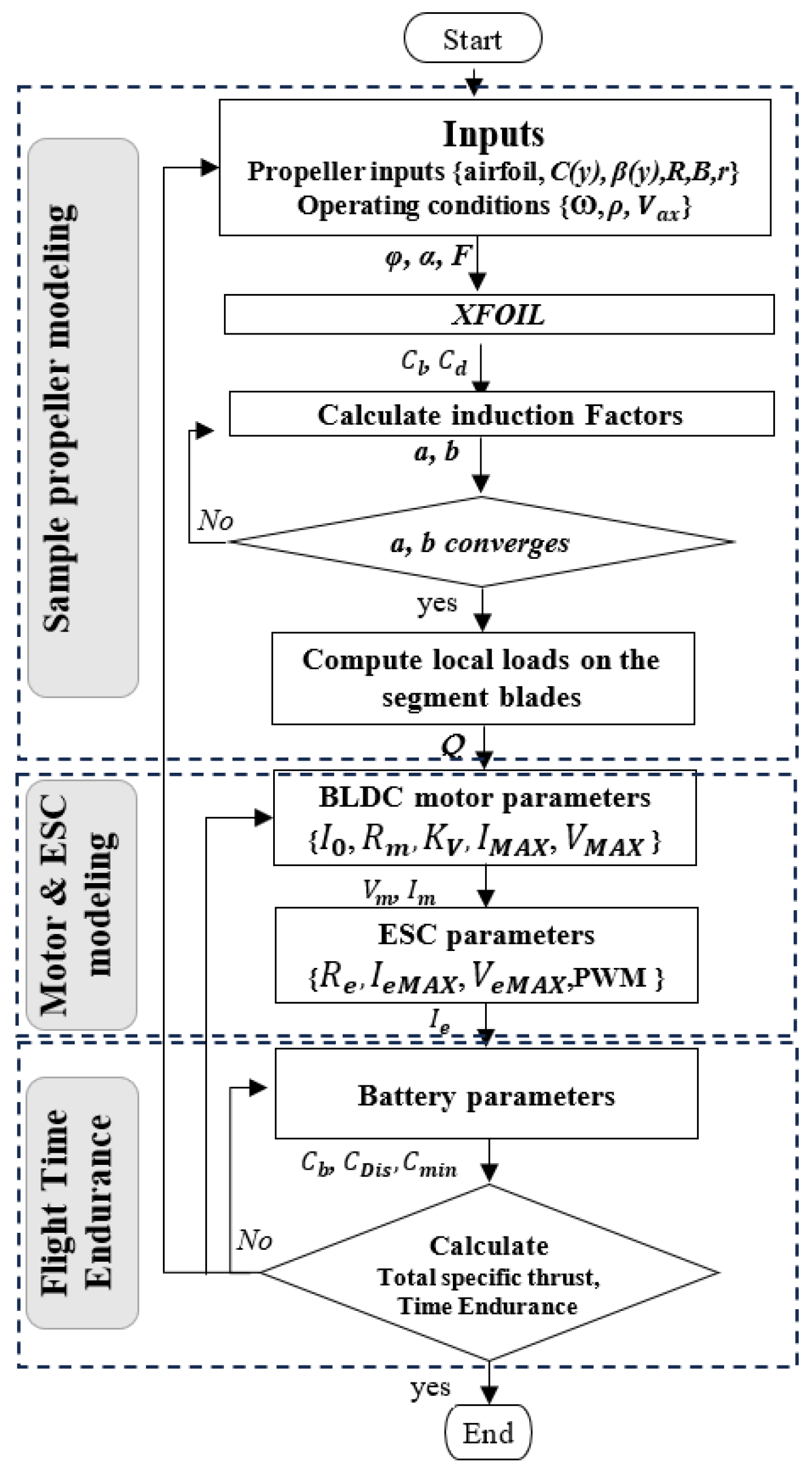
2. Overall Process

The proposed process to select the motor and propeller combination is illustrated in Figure 1. The primary objective of this process is to estimate the flight endurance of the aircraft of interest. To achieve this, the process begins with modeling the candidate propeller, focusing on estimating the thrust and torque. Subsequently, the motor is modeled to calculate the drawn current based on the propeller’s performance. Finally, by modeling the battery, the flight endurance of the aircraft can be accurately estimated. A set of initial guesses for the candidate propeller is determined based on the required thrust and the geometric limitations. As illustrated in Figure 1, the proposed process is iterative in nature.

It involves analyzing a sequence of propeller–motor combinations, which guides the selection of the optimal configuration. To estimate the flight time endurance of the UAV propeller performance in both static and dynamic operating conditions, we use an enhanced blade element momentum theory (EBEMT) model. The input parameters for this step are the propeller’s geometric data, including the segment’s blade (twist angle distributions ($\beta$), chord length (C), number of blades (B), propeller radius (R), and airfoil parameters). The operating condition parameters used in the analysis are the air density ($\rho$), the propeller angular speed ($\omega$), and its free-stream axial velocity ($V_{ax}$). With the set of parameters, the inflow factors ($a,b$) are initialized, the tip loss factor (F) is calculated, and the effective angle of attack ($\alpha$) is computed. Then, the input parameters, as well as the angle of attack, are provided to the XFOIL [9] to estimate the aerodynamic coefficient at each element of the blade. The next step is to check whether the induction factors converge to a certain tolerance. Finally, the localized loads acting upon the blade elements are computed. This computational process facilitates the comprehensive determination of the aggregated parameters, encompassing the thrust, torque, power output, and overall efficiency within the context of the brushless direct current (BLDC) motor model. Concurrently, the electrical attributes of the BLDC motor, the current ($I_m$) and voltage ($V_m$), are derived based on the propeller’s mechanical power and RPM. This intricate interplay culminates in the evaluation of the motor’s efficiency. Additionally, a temporal analysis is conducted to ascertain the endurance duration applicable to the analyzed motor–propeller combination for the given battery parameters, while judiciously considering the pertinent operational circumstances.

3. UAV Propulsion System

3.1. Propeller Modeling

Due to the large number of airfoil profiles that can be selected for a specific aircraft design, it is extremely hard to select what could be considered the optimal propeller. Although a new propeller could be designed for the specific aircraft, such work is time-consuming; thus, propeller selection is preferred. However, in order to select a propeller, it is necessary to know several requirements including the propeller diameter, the flight speed, the propeller rotational speed, the number of propeller blades, the required thrust, and the necessary aerodynamic parameters, e.g., drag, air density, etc.

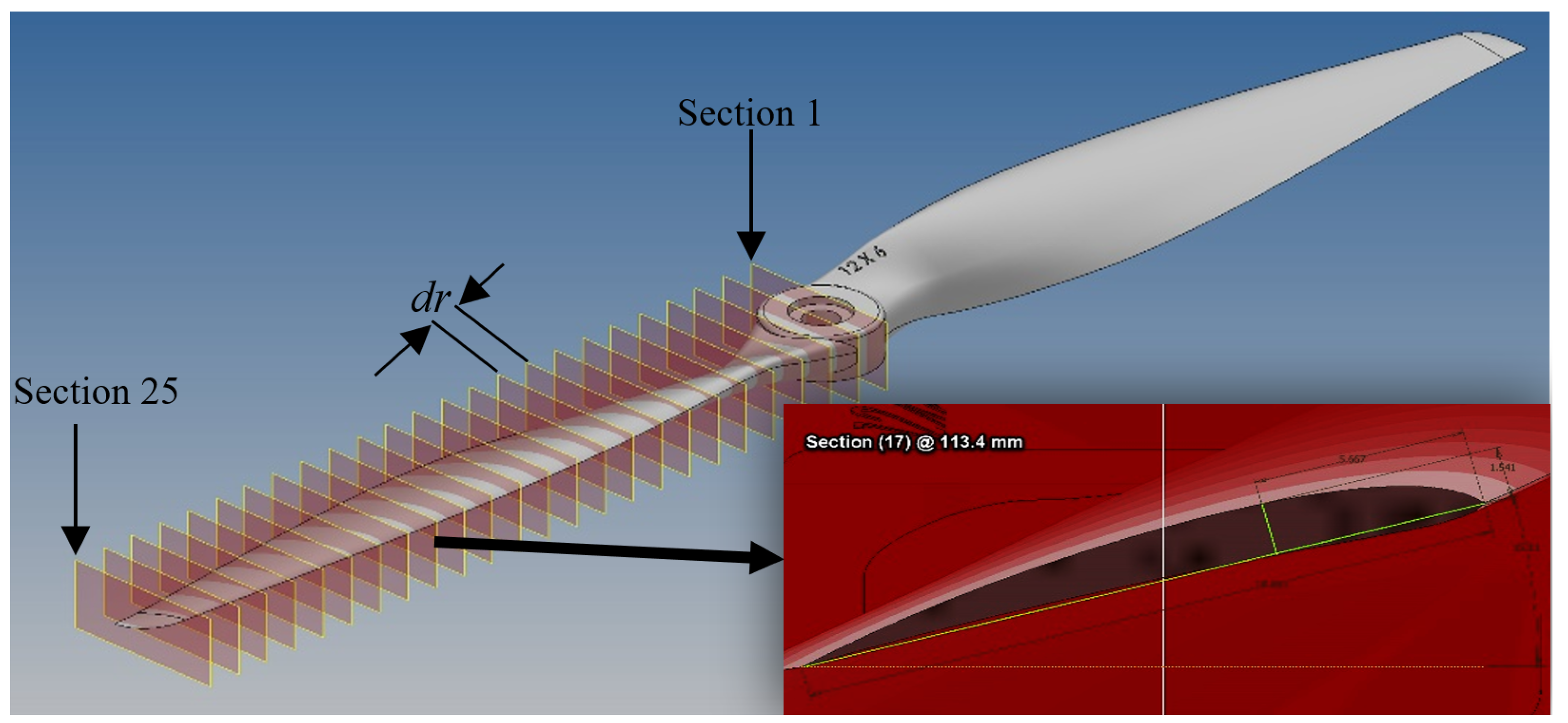
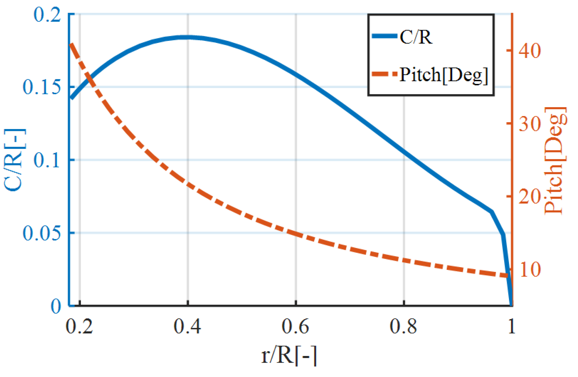
3.1.1. The Propeller Geometrical Data

To facilitate the evaluation of the propulsion system, the geometrical shape of the airfoil cross sections along the span of the blade is used via discrete data points. This mechanism enables the assessment of the aerodynamic performance at each section, and as a result, a complex propeller profile can be analyzed. The discretization process of the propeller, illustrated in Figure 2, encompasses a total of “n” radial stations where “n” can be defined by the user based on the needed accuracy. As an example, if one is using a $12X6E$ propeller, and n = 25, then it is possible to analyze the blade cross sections every 6.1 mm to identify the airfoils. The chord length C and the twist angle $\beta$, along the radial location $r/R$, affect the propeller’s lift and drag characteristics, the angle of attack, the Reynolds number $R_e$, and the Mach number M, as shown in Figure 3.

With these parameters, the propeller’s aerodynamic performance is computed in Section 3.1.2 and Section 3.1.3.

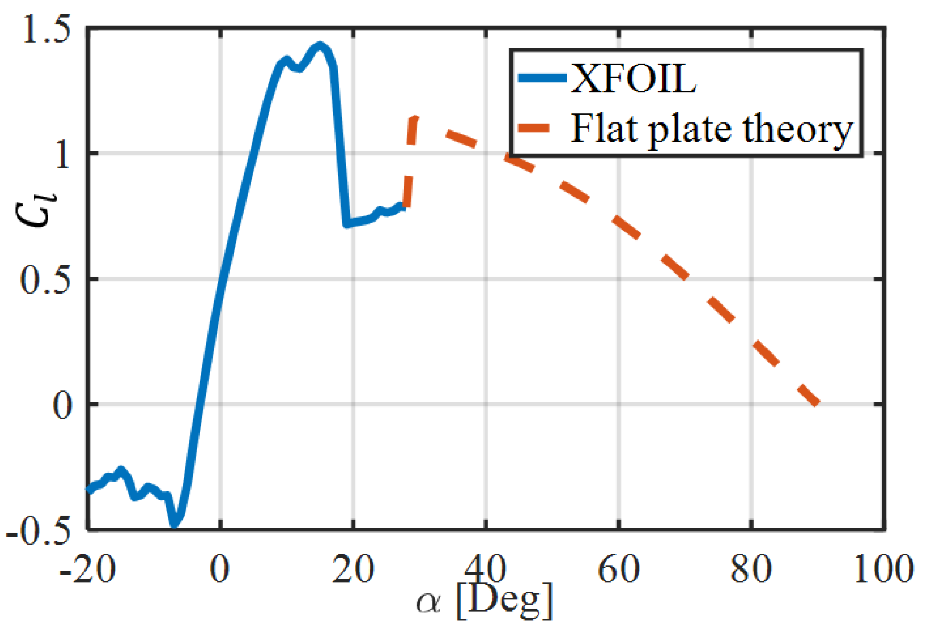
3.1.2. Propeller Aerodynamic Coefficients

In this paper, the local Reynolds number $R_{e_j}$ is calculated at each blade section having the chord $C_j$ and local velocity $V_{l_j}$ [10], as per Equation (1)

$$R_{e_j}={\displaystyle \frac{\rho V_{l_j}{C}_j}{\mu }},$$

(1)

where j is the number of element sections, $\mu$ is the dynamic viscosity, $\rho$ is the air density obtained from the International Standard Atmosphere (ISA) model [11], and $V_l$ is the local velocity computed based on Equation (2).

$$V_{l_j}=\sqrt{V_{a{x}_j}^2+{\left(\omega R_i\right)}^2}$$

(2)

The propeller angular velocity $\omega$ is calculated according to Equation (3).

$$\omega ={\displaystyle \frac{2·\pi ·RPM}{60}}$$

(3)

The computed $R_{e_j}$ and the propeller NACA airfoil at each section for the given propeller are provided to XFOIL, which estimates the following 2D aerodynamic coefficients: (i) the airfoil lift coefficient $C_l$ and (ii) the drag coefficient $C_d$, where XFOIL considers the compressibility and friction effects within the angle of attack $\alpha$ range from −20 to 25 [Deg]. To compute $C_l$ and $C_d$ beyond this range, an empirical approach is used to extrapolate post-stall sectional airfoil performance. This approach is grounded in the flat-plate methodology developed in [12], where a lookup table is used for the segments’ aerodynamic characteristics. Figure 4 and Figure 5 display an illustration of the sectional lift coefficient and drag coefficient plotted against the angle of attack including a linear, nonlinear, and post-stall zone.

3.1.3. Blade Element Momentum Theory (BEMT)

The propeller thrust and moment characteristics are calculated by modeling the axial and circumferential airflow, where the propeller blade is divided into k annular elementary segments, where k is determined based on the available geometrical data as described in [13]. The aerodynamic characteristics of each element comprising the given propeller, considered an infinite wing, are predicted using the local chord angle of attack. The aerodynamic interaction between the various blades comprising the propeller is neglected [14]. The local velocity vector, $V_l$, for each segment comprises the tangential airflow velocity $V_{\theta }$ and the axial velocity $V_{ax}$. This local velocity $V_l$ generates the angle of attack $\alpha$ with the airfoil chord, where each segment of the given propeller is defined at a given geometric incidence angle $\theta$ as represented in Figure 6. The angle between the lift vector $\Delta L_j$ and thrust vector $\Delta T_j$ is defined as the relative inflow angle $\varphi$ computed based on Equation (4).

$$\begin{array}{cc}\hfill & {\phi }_j=ta{n}^{(-1)}(V_{a{\chi }_j}/V_{{\theta }_j})\hfill \\ \hfill & {\alpha }_j={\theta }_j-{\phi }_j\hfill \end{array}$$

(4)

Then, it is possible to compute the elemental thrust $\Delta T_j$ and circumferential force $\Delta F_{{\theta }_j}$, as per Equation (5).

$$\begin{array}{cc}\hfill & \Delta T_j=\Delta L_j\times cos{\phi }_j-\Delta D_j\times sin{\phi }_j\hfill \\ \hfill & \Delta F_{{\theta }_j}=\Delta D_j\times cos{\phi }_j+\Delta L_j\times sin{\phi }_j\hfill \end{array}$$

(5)

The torque required to turn the element of the blade is calculated, as per Equation (6), while the lift and drag forces ($\Delta L_j$, $\Delta D_j$) for each element are computed based on Equation (7).

$$\Delta Q_j=r_j\times \Delta F_{{\theta }_j}$$

(6)

$$\begin{array}{cc}\hfill & \Delta L_j=0.5C_{l_j}\rho V^2\times C_j\times dr\hfill \\ \hfill & \Delta D_j=0.5C_{d_j}\rho V^2\times C_j\times dr\hfill \end{array}$$

(7)

Consequently, the thrust and torque per element are computed per Equation (8).

$$\begin{array}{cc}\hfill & \Delta T_j=0.5\rho {V_j}^2\times (C_{l_j}\times cos{\phi }_j-C_{d_j}\times sin{\phi }_j)B\times C_j\times dr\hfill \\ \hfill & \Delta Q_j=0.5\rho {V_j}^2\times (C_{l_j}\times sin{\phi }_j+C_{d_j}\times cos{\phi }_j)B\times C_j\times dr\times r_j\hfill \end{array}$$

(8)

The total thrust and total torque of the propeller can then be calculated using Equation (9).

$$\begin{array}{cc}\hfill & T={\sum }_1^k\Delta T_j\hfill \\ \hfill & Q={{\sum }_1^k\Delta Q}_j\hfill \end{array}$$

(9)

With the set of the parameters computed via Equations (2)–(4) (i.e., $V_j$, $C_{l_j}$, $C_{d_j}$, ${\alpha }_j$, and ${\varphi }_j$), it is possible to compute the propeller’s total thrust and torque. However, the classical blade element theory is unable to find a relation from where such parameters can be estimated. Therefore, we developed a way to predict the required inflow factors.

Furthermore, to compute the required thrust and torque coefficients, the needed parameters are computed via an iterative process outlined for each element in Equation (10), which comprises the propeller of interest from where the total thrust and torque are obtained via Equation (9).

$$\begin{array}{cc}\hfill & \Delta T_j=4\pi r_j\rho V_{\circ }^2\left(1+a_j\right)a_j·dr\hfill \\ \hfill & \Delta Q_j=4\pi {r_j}^3\rho V_{{ }^{\circ }}\omega \left(1+a_j\right)b_j·dr\hfill \end{array}$$

(10)

Then, the resultant velocity $W_j$ is calculated considering the induction factors per Equation (11).

$$W_j=\sqrt{{\left(\omega ·r_j\left(1-b_j\right)\right)}^2+{\left(V_{{ }^{\circ }}·\left(1+a_j\right)\right)}^2}$$

(11)

The original BEMT theory does not take into account the influence of free vortices that flow at the tip of the propeller from the lower to the upper surface, as shown in Figure 7. These tip vortices create helical formations in the wake, which significantly affect the induced velocity distribution and the angle of attack $\alpha$ along the propeller span. Fortunately, Prandtl described an approximate loss factor F, which includes these propeller tip losses, per Equation (12), which provides the required information.

$$\begin{array}{cc}\hfill & F_j={\displaystyle \frac{2}{\pi }}·{cos}^{-1}\left(e^{-f}\right)\hfill \\ \hfill & f_j={\displaystyle \frac{B}{2}}·{\displaystyle \frac{R-r_j}{r_j·sin{\phi }_j}}\hfill \end{array}$$

(12)

Thus, modifying Equation (10), via Equation (12), to each propeller blade element, as shown in Equation (13), we can approximate the required quantities.

$$\begin{array}{cc}\hfill & \Delta T_j=4\pi r_j\rho V_{{ }^{\circ }}^2\left(1+a_j\right)a_j·F_j·dr\hfill \\ \hfill & \Delta Q_j=4\pi {r_j}^3\rho V_{{ }^{\circ }}\omega \left(1+a_j\right)b_j·F_j·dr\hfill \end{array}$$

(13)

For tip Mach numbers up to 0.6, the velocity will undergo a rise in the gradient of the lift curve 2D airfoil. This change is estimated using Glauert’s Mach correction factor, per Equation (14), which provides the required value.

$$\begin{array}{c}\hfill C_l={\displaystyle \frac{C_{l\to M=0}}{\sqrt{1-M^2}}}\end{array}$$

(14)

The total thrust and total torque are determined using Equation (9), which account for both the inflow factor and the Mach number. The BLDC plays a pivotal role in this setup, as it is responsible for driving the propeller. The mechanical power output from the propeller serves as the input to the BLDC motor model, enabling a comprehensive analysis of the motor’s performance and efficiency under various operating conditions.

3.2. BLDC Motor Modeling

With the aspects obtained from the BEMT analysis, the BLDC motor model can now be formulated to predict the required motor voltage $V_m$ and current $I_m$ and, subsequently, calculate the motor efficiency. In this respect, the BLDC motor model is coupled from the propeller model to enable easily acquiring the mechanical power $P_{mech}$; for this, we formulate a motor model using the propeller torque $Q_m$ and the propeller angular velocity $\omega$ as inputs and the motor parameters. The BLDC motors are thus modeled as a traditional DC motor, as illustrated in Figure 8, where $R_m$ is the motor resistance, EMF is the back electromotive force, and $I_0$ is the motor idle current. The motor parameters [$I_0$,$R_m$,$K_v$] can be obtained by the manufacturers or be measured with the proposed experimental setup in Section 4. Based on the power balance concept, the total electrical power transferred to the motor can be computed using Equation (15), where $P_{Elect}$ is the total electrical power and $P_{copper}$ and $P_{iron}$ are the copper and iron losses of power, respectively, calculated via Equation (16).

$$\begin{array}{c}\hfill P_{Elect}=P_{copper}+P_{iron}+P_{mech}\end{array}$$

(15)

$$\begin{array}{cc}\hfill & P_{copper}=I_m^2{R}_m\hfill \\ \hfill & P_{iron}=V_m{I}_0-I_0^2{R}_m\hfill \end{array}$$

(16)

The motor efficiency ${\eta }_{motor}$ can be obtained via Equation (17).

$$\begin{array}{c}\hfill {\eta }_{motor}={\displaystyle \frac{P_{mech}}{P_{Elect}}},\end{array}$$

(17)

and with the motor’s current, the rest of the interested parameters can be obtained. Consistent with the motor current, $I_m$ is calculated based on Equations (18)–(20).

$$\begin{array}{c}\hfill K_E={\displaystyle \frac{V_0-I_0{R}_m}{K_V{V}_{m0}}},\end{array}$$

(18)

where $K_E$ is the EMF constant.

$$\begin{array}{c}\hfill K_T={\displaystyle \frac{30}{\pi }}{K}_E,\end{array}$$

(19)

where $K_T$ is the motor torque constant. The motor current $I_m$ and voltage $V_m$ are defined via (20):

$$\begin{array}{cc}\hfill & I_m={\displaystyle \frac{Q}{K_T}}+I_0\hfill \\ \hfill & V_m=K_{E}n+I_m{R}_m.\hfill \end{array}$$

(20)

3.3. Modeling of the Electronic Speed Controller

The electronic speed controller (ESC) is a typical device used to drive BLDC motors, typically used in electrically powered drones. The ESC can be modeled as a device that transfers a certain percentage of the input voltage to the motor based on the throttle command. This throttle command is translated into the ESC’s duty cycle, per Equation (21).

$$\begin{array}{cc}\hfill & V_{ESC}=\mathrm{Duty}\mathrm{Cycle}\times V_b\hfill \\ \hfill & V_m=V_{ESC}-I_m{R}_{ESC},\hfill \end{array}$$

(21)

where $R_{ESC}$ is the resistance value from the input to the output of the ESC when the path is activated; according to this study [15], the $R_{ESC}$ range is 9 to 45 mΩ. Consequently, the ESC current is calculated through Equation (22).

$$\begin{array}{c}\hfill I_{ESC}=\mathrm{Duty}\mathrm{Cycle}\times I_m\end{array}$$

(22)

In this research, the efficiency of the ESC is assumed to be $100\%$, due to the high efficiency of the ESC model used. When selecting ESCs, the maximum rated amperage is the primary parameter. It is crucial to choose an ESC with a maximum rated amperage that is significantly higher than the required drive current per motor. This ensures that the field-effect transistors (FETs) within the ESC do not overheat and fail due to excessive current demands, providing an ESC with a sufficient current rating,

3.4. Battery Modeling

The primary objective of battery modeling is to accurately calculate the flight endurance of a system and ensure that the battery can sustain the maximum current required. This simplified model facilitates easier analysis and calculation of the battery’s behavior during the discharge process. It is important to note that this research does not specifically study the impact of temperature on battery performance. Temperature is a significant factor that can affect a battery’s behavior, including its capacity, internal resistance, and overall performance. Undoubtedly, one of the most crucial parameters in battery selection is the battery capacity $C_b$, which represents the amount of energy the battery can store. The capacity directly affects the endurance time $T_{Endurance}$ of a system powered by the battery, per Equation (23).

$$\begin{array}{c}\hfill T_{Endurance}={\displaystyle \frac{C_b-C_{min}}{I_b}}·{\displaystyle \frac{60}{1000}}\left[\min \right],\end{array}$$

(23)

where $C_{min}$ is the battery minimum capacity, and $I_b$ is the battery current. Additionally, the discharge rate $C_{Dis}$ is another significant parameter to consider. It refers to the maximum current that the battery can deliver continuously without significantly affecting its performance or causing damage. Choosing a battery with a discharge rate that meets or exceeds the maximum current requirements of the system is essential to ensure proper operation and prevent issues such as voltage drop or overheating.

4. Experimental Setup

This section focuses on the complete description of the experiment, which was used to measure the aerodynamic properties of the propellers to validate the high-fidelity CFD models, BEMT in static conditions, and the BLDC motor model. The main objective of the experiment is to measure the thrust of the propeller under static conditions, as a counterpart to the propeller RPM, voltage, and current. As a consequence, a special test stand was designed as illustrated in Figure 9. To use the full potential of the experimental equipment and to perform static tests, the sensors were placed in the measuring head illustrated in Figure 10, which consisted of the selected propeller, the BLDC, the Hall effect encoder, and the load cell. An effort was made to decrease the test rig complexity and the measurement disruptions by fixing the load cell, according to the propeller’s expected thrust, using a 3D printing design, by measuring the bending distortion.

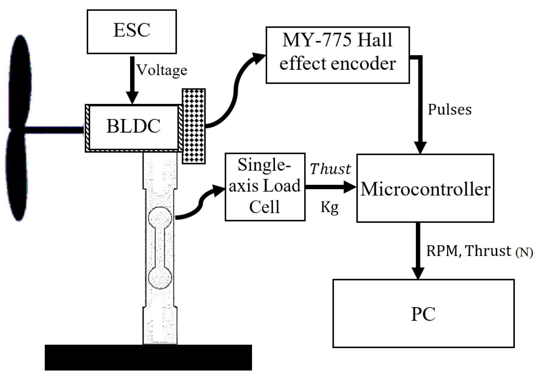
4.1. Thrust Measurement

TAL220 load cell (HT Sensor Technology, Straight Bar, 10 kg of full scale) was used to measure the propellers’ thrust. This load cell has a maximum capacity of 10 Kg connected to a 24-bit ADC and signal conditioning module based on an HX711chip to amplify the load cell output, in addition to converting to digital form and then sending the reading to the microcontroller using the serial communication. Before using the load cell assembly for any tests, load cell calibration took place, where the axial load that represented the propeller thrust on the load cell was created using calibrated weights $\{1,2,3\}$ Kg. The thrust and voltage were found to be linearly related by varying a known force applied to the load cell with ±2 g of tolerance per kilogram after calibration. The thrust–speed curve in Figure 11 shows the experimental result of the static thrust exhibiting a parabolic variation with the RPM, as affirmed in other studies [2,16].

4.2. Propeller Rotation Speed Measurement

An MY-775 two-channel Hall effect encoder was utilized to detect the rotation of a magnetic disc mounted on the motor’s back shaft, as depicted in Figure 10. The encoder provides seven TTL pulses per mechanical revolution of the motor shaft. The propeller rotational speed was obtained by counting the number of pulses the shaft made in a fixed time interval using a microcontroller; after calculating the number of pulses per second, the RPM was estimated easily by multiplying it by 60. The output voltages and response time of the encoder proved to be enough for precise rotation speed measurements because the tested propeller’s rotational speed never surpassed 10,000 [RPM]. The pulses that were counted by the microcontroller were also measured using an oscilloscope for a confident result.

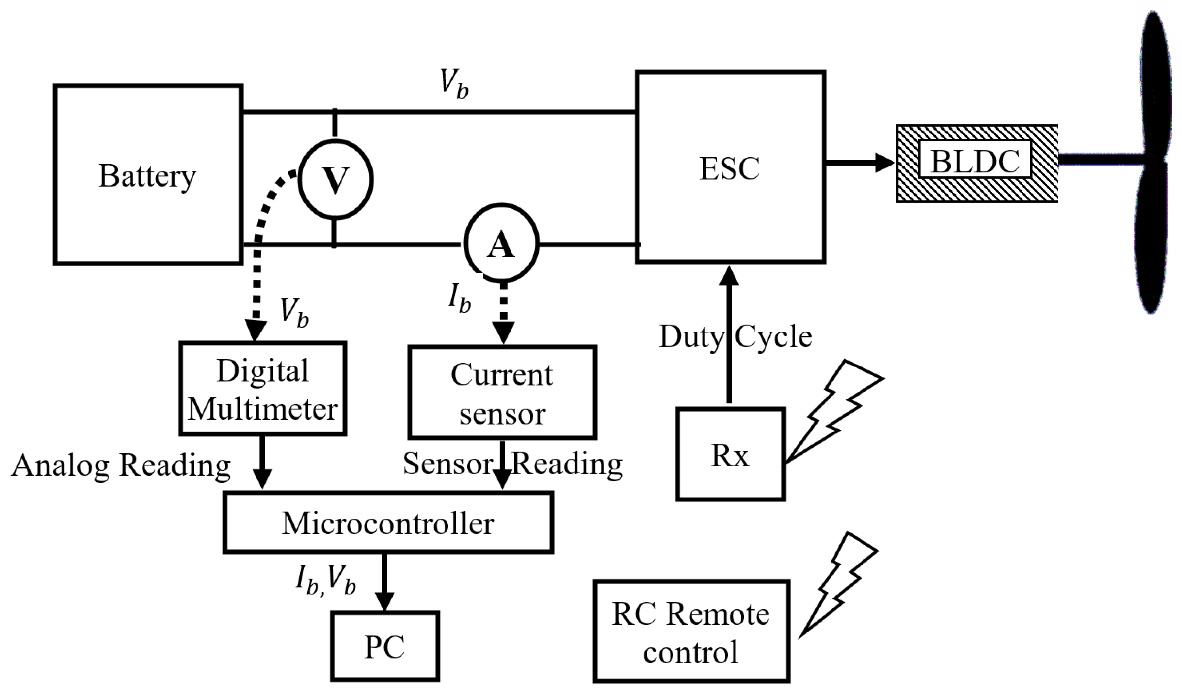
4.3. BLCD Electrical Power Measurement

The BLDC (ECO 2826C) is energized using a three-cell battery and ESC to control the motor speed to calculate the motor efficiency, and the power consumption was measured. In this regard, the battery voltage was measured using a digital multimeter, and the Current Sensor ACS712 was used to measure the current, which was validated with a clamp-on ammeter. All the measured data were sent to the microcontroller synchronized with head block sensors. Eventually, the microcontroller sent the recorded measurement to the PC, as shown in Figure 12. The current–speed curve and the BLDC motor efficiency in Figure 11 illustrate the experimental result of the measured electrical and mechanical power of the motor represented by the best polynomial fitting.

5. Computational Fluid Dynamics Analysis

Computational fluid dynamics, or CFD, is a powerful tool for studying aerodynamics in a variety of applications, including the modeling of small-scale rotating propellers. The literature contains several studies that examine and validate the aerodynamic characteristics of quad-rotor UAV propellers using computational fluid dynamics [17,18,19,20]. The purpose of the CFD analysis in this study is to determine the aerodynamic performance and parameters to set the propeller mathematical model. Specifically, a fixed zone and rotating zone portions made up the computational domain. Incompressible and turbulent flow assumptions were applied when using the offset mesh approach. A k-Omega SST turbulence model with curvature correction was used in the analyses, which were carried out using a Navier–Stokes solver (Ansys CFXv19). A variety of tasks may be accomplished with the use of propeller CFD models, such as improving the propeller design, studying the impacts of various blade shapes, determining how operational circumstances affect the performance, and determining how the propeller interacts with the surrounding flow field. Without the need for costly experimental testing or physical prototypes, engineers may obtain a better knowledge of the aerodynamic properties of propellers by running CFD simulations. This makes design iterations quicker and more affordable, enhances the overall effectiveness and performance of a propeller-driven item, and helps to implement the propulsion system mathematical model.

5.1. Computational Fluid Dynamics Model

The electric propeller was an APC 12 × 6 Thin. The pultrusion technology used in the production of APC propellers enables a greater fiber (60%)-to-resin (nylon binder) density. Compared to glass-filled nylon, this offers noticeably more strength and stiffness. Controlling vibration resonance response is easier with the extra rigidity. Because of the increased strength, smaller cross sections may be used, which is advantageous for weight and aerodynamic efficiency. The computer-optimized design of these props results in a quieter appearance. For increased production and longer life, the lightweight molded nylon structure lowers the spinning mass. Using reinforcing fibers helps provide a consistent accurate pitch at any RPM. It has a 305 mm outer diameter and a 20 mm hub diameter. The CAD model of the propeller is shown in Figure 2.

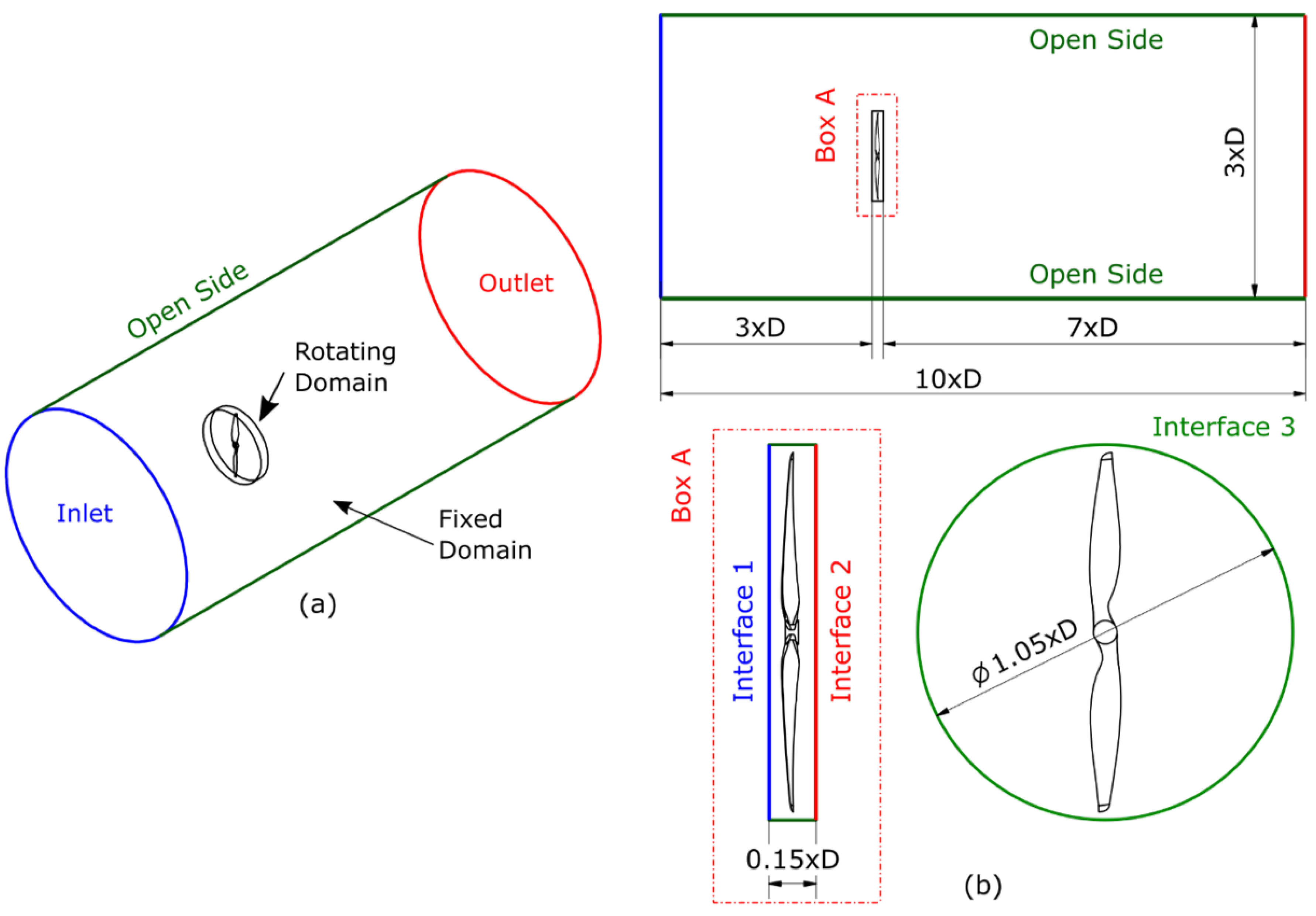
5.2. Computational Fluid Dynamics Domain

The CFD domain consisted of two parts: the rotor (rotating frame of reference) and the surrounding atmosphere (fixed frame of reference). The CFD domain dimensions and all boundary types are represented in Figure 13.

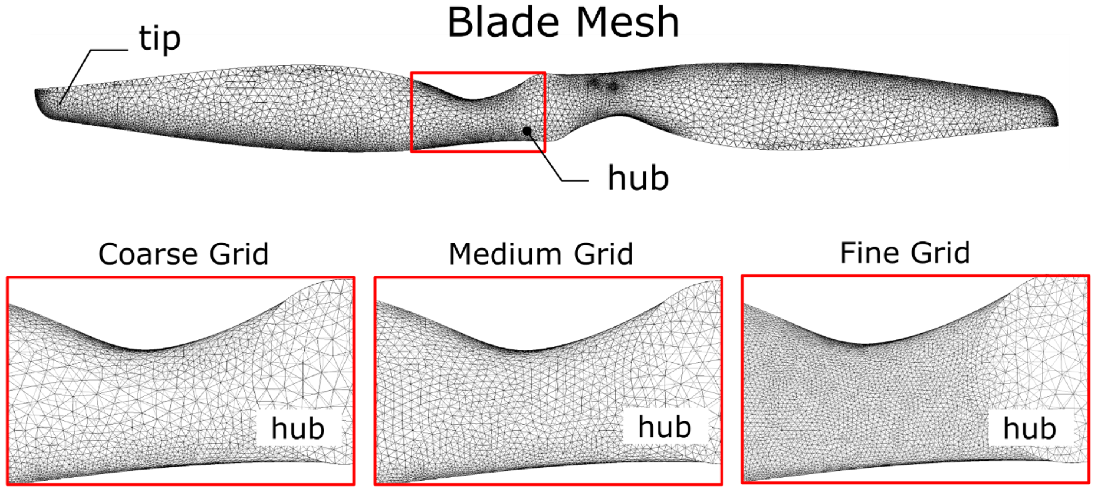
5.3. Computational Fluid Dynamics Mesh

The CFD domains were meshed using an unstructured grid with three different sizes: coarse, medium, and fine grid, as shown in Figure 14. After performing a mesh sensitivity analysis, the medium grid showed that the propeller performance was independent of the grid size.

5.4. Computational Fluid Dynamics Results and Validation

Regarding validating the CFD simulation, a comparison between the experimental data and CFD results was performed, as shown in Figure 15. This comparison showed a good agreement between both results. Therefore, the CFD model estimated the static torque and the figure of merit, FOM; furthermore, in Figure 16, we provide the dynamic coefficients for the thrust, torque, power, and propeller efficiency. These results were used to validate the BEMT model.

6. Results

This section presents the comparative analysis and validation of outcomes acquired through the utilization of the proposed sub-system mathematical models, especially the propeller BEMT. These results are juxtaposed with experimental data and CFD to establish a balance between the computational accuracy and the computational complexity.

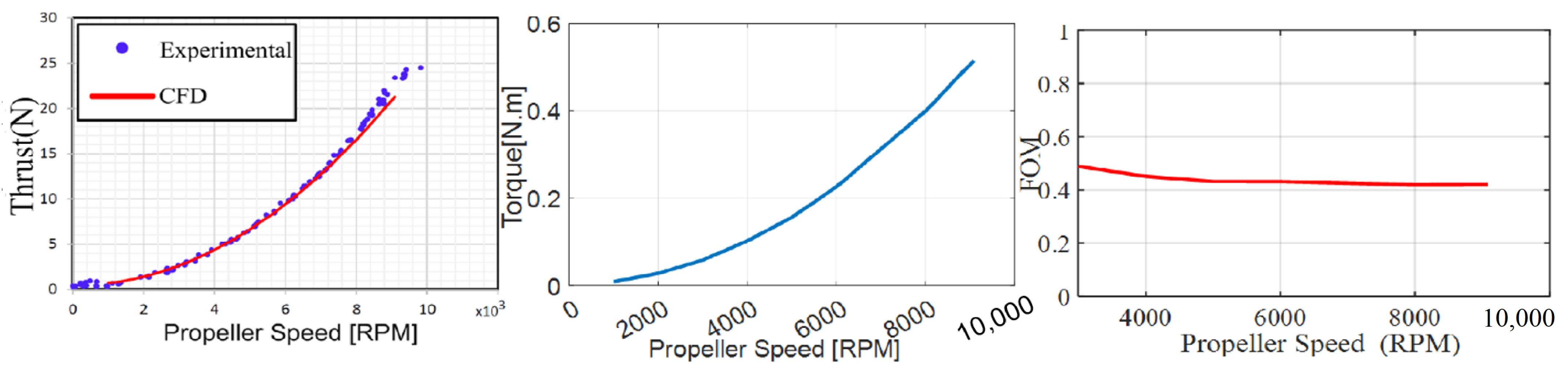
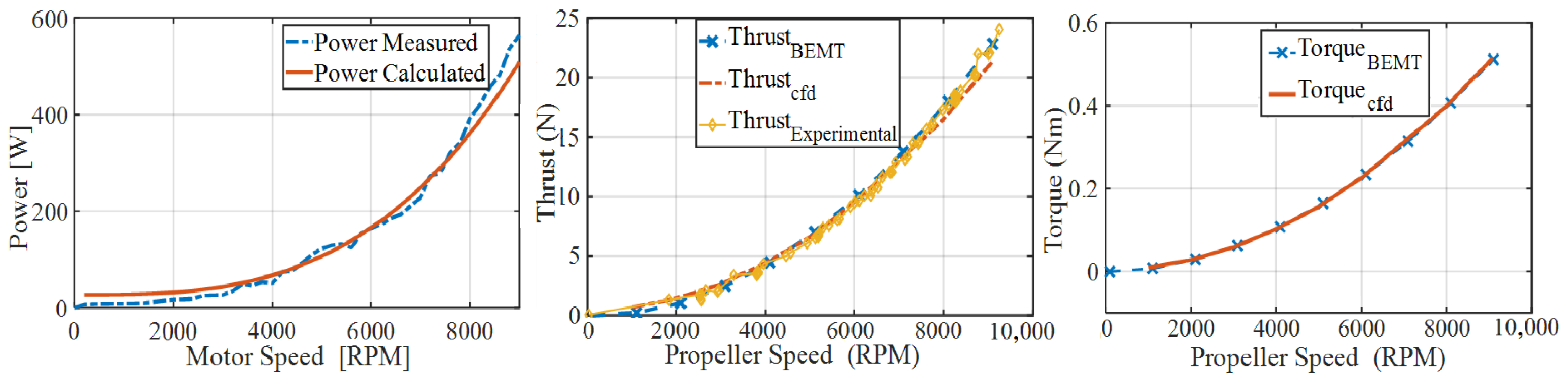
6.1. Static Performance Validation

The propulsion system was statically validated by comparing the simulated static thrust and torque for the propeller and motor voltage and current versus its rotational speed [RPM] against the CFD and experimental results. As depicted in Figure 17, it is clear that when the RPM increases, the thrust, torque, and motor electrical power increase. It is worth noting that the comparative evaluation of the motor electrical power and the estimated thrust and torque values derived from the blade element momentum theory (BEMT), in contrast to the experimental and CFD-derived data, manifests an impressive degree of concurrence. This convergence underscores the BEMT’s adeptness in effectively appraising the static performance across the the RPM range under scrutiny.

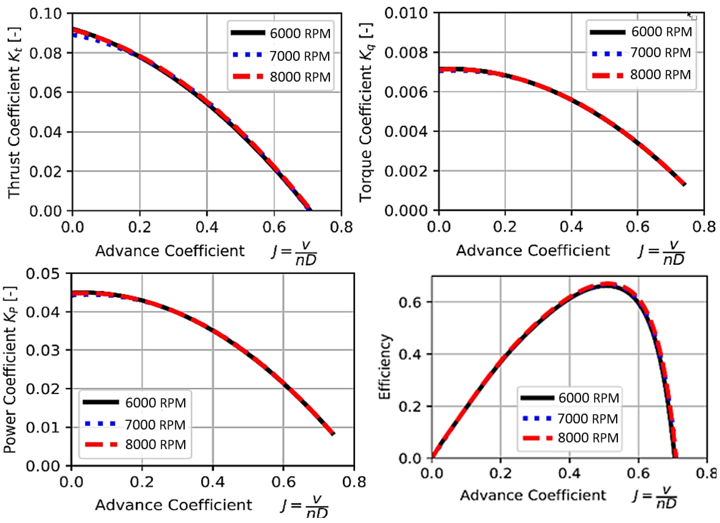
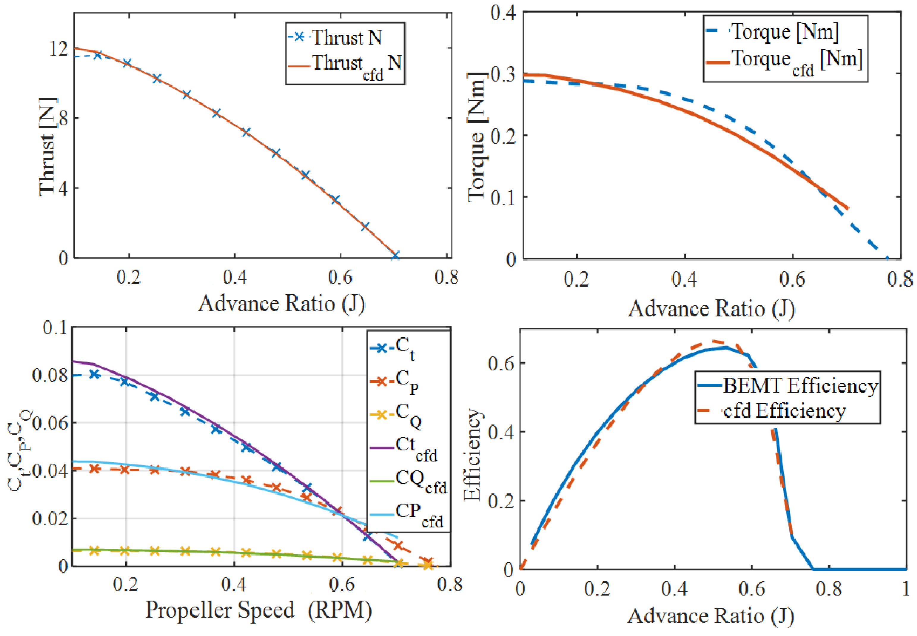
6.2. Dynamic Propeller Performance at Different Advance Ratios

In light of the preceding insights into the static performance, the optimal rotational velocity for the propeller was identified as 7000 RPM, aligning with the experimental observations. This particular rotational velocity of 7000 RPM was selected as the focal point for subsequent investigations. Figure 18 shows the variation in the propeller thrust and torque (Ct, Cp, CQ ) coefficients and the propeller efficiency versus a range of the advance ratio J, where the overall trend for the estimated BEMT and the high fidelity CFD showed a good agreement. This elucidates that the produced thrust and torque influenced the forward velocity to the extent that these forces decreased to zero at an advance ratio around J = 0.7. The figure illustrates that the BEMT succeeded in estimating the thrust and torque; however, the torque was overestimated with a negligible value in the range of J = 0.3 and J = 0.6. Moreover, Figure 18 shows the variation in the propeller’s efficiency $\eta$ versus the advance ratio J. It is clear that the curves of the $\eta$ obtained from the BEMT were underestimated and influenced by the torque trend; however, it remained generally consistent. The efficiency peak was obtained from both methods, the BEMT at J = 0.53 and the CFD at J = 0.51 (i.e., freestream velocity $V_{ax}$ = 17.5 m/s).

6.3. Propulsion System Efficiency

The effectiveness of the propulsion system as a whole is largely contingent upon the agreeable pairing of the motor and propeller components. The total specific thrust was computed to assess the total efficiency of the motor and propeller.

$$\mathrm{Total}\mathrm{Specific}\mathrm{Thrust}={\displaystyle \frac{\mathrm{Propeller}\mathrm{Thrust}\left[\mathrm{g}\right]}{\mathrm{Motor}\mathrm{Electrical}\mathrm{Power}\left[\mathrm{W}\right]}}$$

given that both the thrust of the propeller and the efficiency of the motor are not constant with different operating conditions. Typically, motor manufacturers provide information regarding the overall specific thrust. These data are a valuable resource for understanding the performance characteristics of a given motor. However, the manufacturer furnishes motor performance data concerning the recommended propellers at a few operating speeds under static conditions. Conversely, the proposed model introduces an expansive range of performance data, encompassing static and dynamic assessments, for diverse propellers across varying altitudes. Illustratively, in the case of a motor, the overall specific thrust across diverse states is depicted in

Table 1. Propulsion system model results for the ECO 2212C–830 Kv BLDC motor and the $12\times 6E$ and $13\times 6.5E$ propellers.

Battery Voltage	Propeller	RPM	Current (A)	Elec. Power (W)	Mech. Power (W)	Thrust (N)	Total Specific Thrust (g/w)	Endurance (min)
11.1V(3 S) 5200 mAh	$12\times 6E$	3000	2.27	25.18	18.41	2.3	9.34	116.92
		4000	5.31	58.93	42.96	4.23	7.32	49.95
		5000	10.5	116.6	82.92	6.71	5.87	25.25
		6000	18.59	206.39	142.05	9.77	4.83	14.26
		7000	30.4	337.44	224.1	13.38	4.05	8.72
		8000	46.83	519.82	332.8	17.57	3.45	5.66
		9000	68.88	764.57	471.91	22.32	2.98	3.85
	$13\times 6.5E$	3000	2.46	27.28	19.83	2.96	11.09	107.92
		4000	5.84	64.83	46.64	5.46	8.59	45.41
		5000	11.69	129.72	90.49	8.69	6.83	22.69
		6000	20.86	231.58	155.58	12.66	5.58	12.71
		7000	34.35	381.27	246.08	17.37	4.65	7.72
		8000	53.23	590.81	366.19	22.82	3.94	4.98
		9000	78.69	873.4	520.08	29.01	3.39	3.37

and

Table 2. Propulsion system model results for the ECO 2826C–1080 Kv BLDC motor and the $12\times 6E$ and $13\times 6.5E$ propellers.

Battery Voltage	Propeller	RPM	Current (A)	Elec. Power (W)	Mech. Power (W)	Thrust (N)	Total Specific Thrust (g/w)	Endurance (min)
11.1V(3 S) 5200 mAh	$12\times 6E$	3000	2.47	27.42	18.41	2.3	8.57	107.36
		4000	5.13	56.93	42.96	4.23	7.57	51.71
		5000	9.38	104.12	82.92	6.71	6.58	28.27
		6000	15.67	173.92	142.05	9.77	5.73	16.93
		7000	24.45	271.42	224.1	13.38	5.03	10.85
		8000	36.22	402	332.8	17.57	4.46	7.32
		9000	51.46	571.26	471.91	22.32	3.99	5.15
	$13\times 6.5E$	3000	2.62	29.06	19.83	2.96	10.41	101.32
		4000	5.52	61.25	46.64	5.46	9.09	48.06
		5000	10.2	113.25	90.49	8.69	7.83	25.99
		6000	17.17	190.62	155.58	12.66	6.77	15.44
		7000	26.96	299.26	246.08	17.37	5.92	9.84
		8000	40.12	445.36	366.19	22.82	5.23	6.61
		9000	57.24	635.4	520.08	29.01	4.66	4.63

. This helps the designers select motor–propeller combinations that align with their specific requisites. A higher total specific thrust indicates a more efficient propulsion system, signifying that the system can generate greater thrust per unit of power consumed. By optimizing the motor and propeller combination to achieve the highest possible total specific thrust, designers can design propulsion systems that are simultaneously potent and energy-efficient. Consequently, this optimization extends the system’s endurance, allowing for operation on the same battery capacity. For illustration, a case study is presented using two distinct motors, namely the ECO 2826C–1080Kv and ECO 2212C–830 Kv.

7. Conclusions

This paper proposed a practical method to help designers quickly determine the optimal propulsion system to maximize the efficiency of the propulsion system under the desired flight condition. The parameters that may affect the endurance of fixed-wing UAVs were studied based on a theoretical analysis, which may help designers optimize the parameters for a more efficient design, in the sense that it decomposes the propulsion model into sub-models, with the performance testing and modeling of a motor, electronic speed controller, and propeller. The methodology used for the motor and propeller hardware testing was presented. This research successfully demonstrated the following:

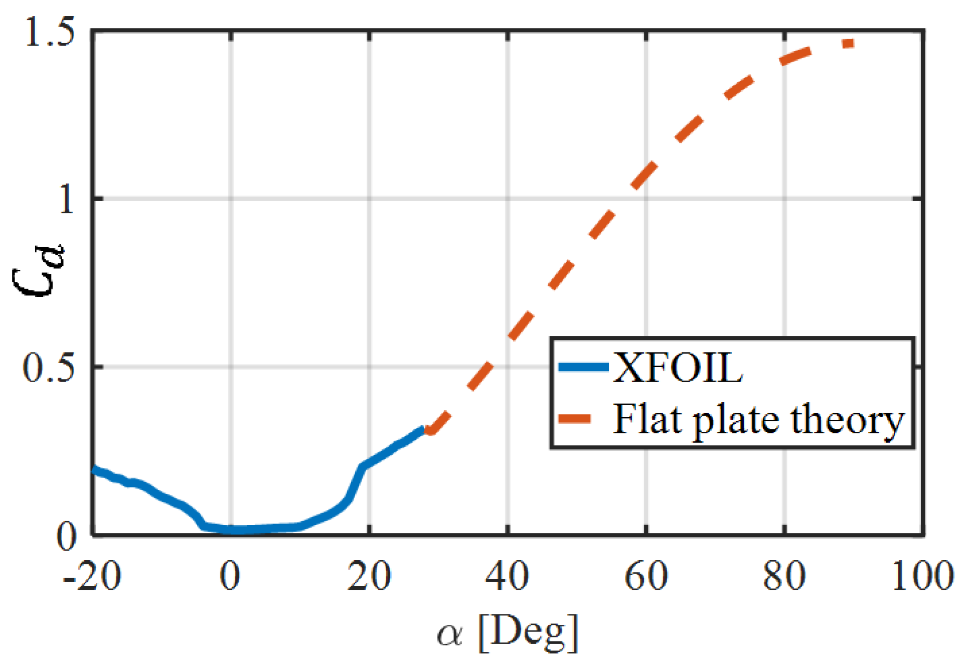
• A comprehensive range of $C_l$ and $C_d$ aerodynamic coefficients in the post-stall zone for the propeller was obtained by integrating XFOIL6.94 software with the flat-plate method. This approach successfully accounted for variations in the Reynolds and Mach numbers, enhancing the accuracy of the aerodynamic predictions.
• The proposed propeller sub-model effectively analyzes static and dynamic performance, as well as airflow properties, under the international standard atmosphere (ISA) model. This provides a reliable framework for predicting propeller behavior in various flight conditions.
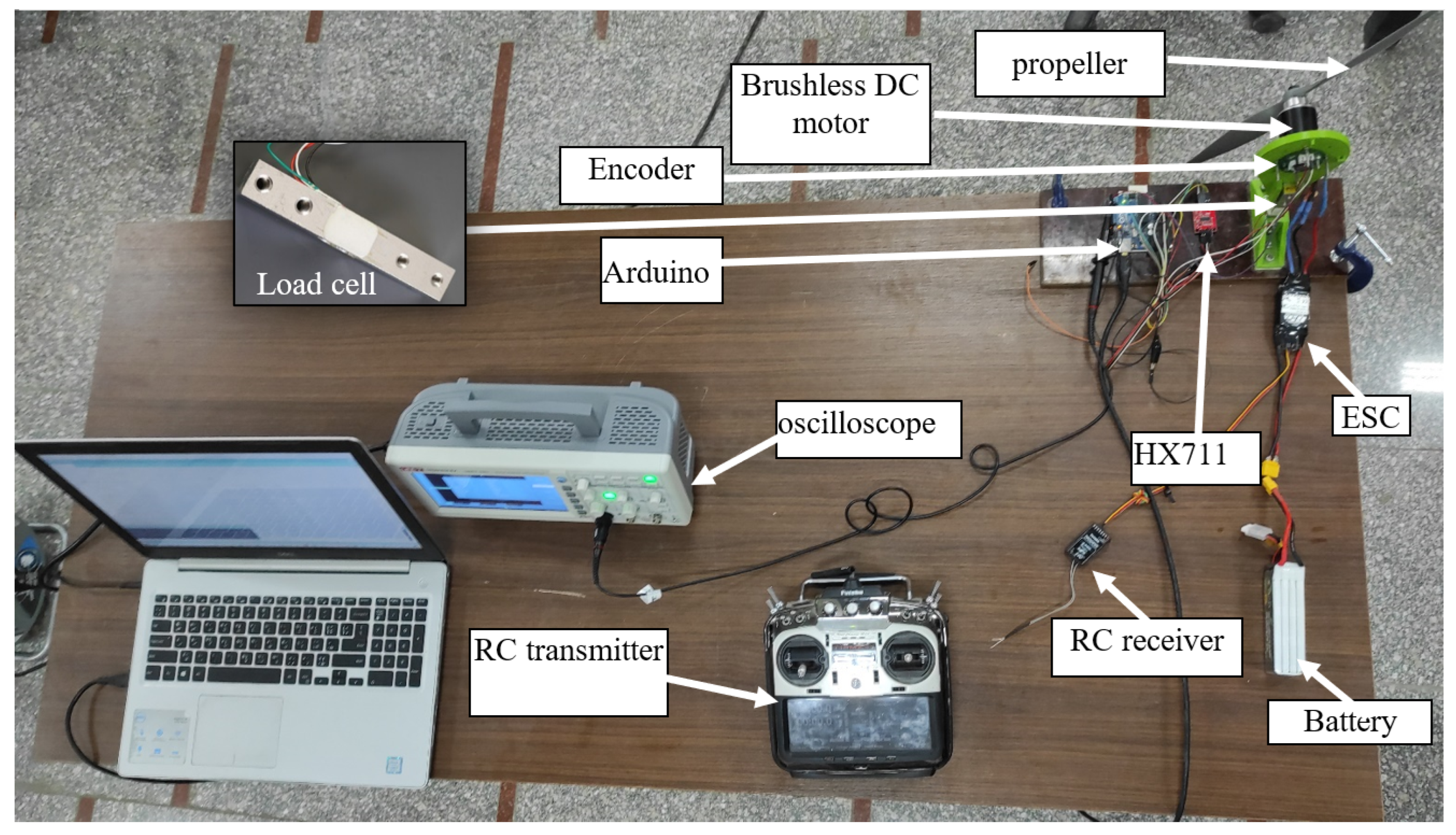
• A test rig was established to validate the CFD and the BEMT model regarding the static performance. Additionally, this setup can be employed for more dynamic performance investigations based on wind tunnels.
• CFD was successfully employed to evaluate the dynamic performance of the proposed low-computational-power model, confirming its effectiveness for real-time applications.
• An extensive analysis of BLDC motor performance was conducted across a wide range of RPMs, offering insights into load versus electrical power cases not typically supported by manufacturers. This analysis fills a critical gap in the existing knowledge, aiding in more accurate motor selection.
• The proposed model takes into account both the maximum discharge current of the battery and the maximum current of the electronic speed controller (ESC), considering the practical constraints and requirements.
• The compatibility between the motor and the propeller significantly influences the endurance; in this regard, the proposed model computes the total specific thrust as a means to assess the overall propulsion system efficiency.

References

- Hoyos, J.D.; Jímenez, J.H.; Alvarado, P. Improvement of electric aircraft endurance through propeller optimization via BEM-CFD methodology. In Proceedings of the Journal of Physics: Conference Series; IOP Publishing: Bristol, UK, 2021; Volume 1733, p. 012011. [Google Scholar]
- Virginio, R.; Fuad, F.; Jihadil, M.; Ramadhani, M.; Rafie, M.; Stevenson, R.; Adiprawita, W. Design and implementation of low cost thrust benchmarking system (TBS) in application for small scale electric UAV propeller characterization. In Proceedings of the Journal of Physics: Conference Series; IOP Publishing: Bristol, UK, 2018; Volume 1130, p. 012022. [Google Scholar]
- Khan, W.; Nahon, M. A Propeller Model for General Forward Flight Conditions; Emerald Group Publishing Limited: Leeds, UK, 2015; Volume 3, pp. 72–92. [Google Scholar]
- Dai, X.; Quan, Q.; Ren, J.; Cai, K.Y. Efficiency optimization and component selection for propulsion systems of electric multicopters. IEEE Trans. Ind. Electron. 2018, 66, 7800–7809. [Google Scholar] [CrossRef]
- Tan, Y.H.; Chen, B.M. Motor-propeller matching of aerial propulsion systems for direct aerial-aquatic operation. In Proceedings of the 2019 IEEE/RSJ International Conference on Intelligent Robots and Systems (IROS), Macau, China, 3–8 November 2019; IEEE: New York, NY, USA, 2019; pp. 1963–1970. [Google Scholar]
- Etewa, M.; Safwat, E.; Abozied, M.A.H.; El-Khatib, M.M. Modeling and systematic investigation of a small-scale propeller selection. J. Eng. Sci. Mil. Technol. 2023, 7, 15–21. [Google Scholar] [CrossRef]
- Elbaioumy, M.K.; Elkhatib, M.M. Modelling and Simulation of Surface to Surface Missile General Platform. Adv. Mil. Technol. 2018, 13, 227–290. [Google Scholar] [CrossRef]
- Gad, M.; Mohamed, M.; Elkhatib, M. Design of an intelligent lateral autopilot for short range surface-to-surface aerodynamically controlled missile. In Proceedings of the 2020 15th International Conference on Computer Engineering and Systems (ICCES), Cairo, Egypt, 15–16 December 2020; IEEE: New York, NY, USA, 2020; pp. 1–8. [Google Scholar]
- Drela, M. XFOIL Users Guide, Version 6.94; MIT Aero Astro Department: Cambridge, MA, USA, 2002. [Google Scholar]
- Liu, X.; Zhao, D.; Oo, N.L. Comparison studies on aerodynamic performances of a rotating propeller for small-size UAVs. Aerosp. Sci. Technol. 2023, 133, 108148. [Google Scholar] [CrossRef]
- Kamal, A.M. Modeling, Analysis and Identification of Airplane Flight Dynamics. Master’s Thesis, Military Technical College (MTC), Cairo, Egypt, 2014. [Google Scholar]
- Tangler, J.; Kocurek, D. Wind turbine post-stall airfoil performance characteristics guidelines for blade-element momentum methods. In Proceedings of the 43rd AIAA Aerospace Sciences Meeting and Exhibit, Reno, NV, USA, 11–12 January 2005; p. 591. [Google Scholar]
- Ledoux, J.; Riffo, S.; Salomon, J. Analysis of the blade element momentum theory. SIAM J. Appl. Math. 2021, 81, 2596–2621. [Google Scholar] [CrossRef]
- McCrink, M.H.; Gregory, J.W. Blade element momentum modeling of low-reynolds electric propulsion systems. J. Aircr. 2017, 54, 163–176. [Google Scholar] [CrossRef]
- Bershadsky, D.; Haviland, S.; Johnson, E.N. Electric multirotor UAV propulsion system sizing for performance prediction and design optimization. In Proceedings of the 57th AIAA/ASCE/AHS/ASC Structures, Structural Dynamics, and Materials Conference, San Diego, CA, USA, 4–8 January 2016; p. 0581. [Google Scholar]
- Rubin, R.L.; Zhao, D. New development of classical actuator disk model for propellers at incidence. AIAA J. 2021, 59, 1040–1054. [Google Scholar] [CrossRef]
- Oktay, T.; Eraslan, Y. Computational fluid dynamics (Cfd) investigation of a quadrotor UAV propeller. In Proceedings of the International Conference on Energy, Environment and Storage of Energy, Xi’an, China, 7–9 August 2020; pp. 1–5. [Google Scholar]
- Penkov, I.; Aleksandrov, D. Analysis and study of the influence of the geometrical parameters of mini unmanned quad-rotor helicopters to optimise energy saving. Int. J. Automot. Mech. Eng. 2017, 14, 4730–4746. [Google Scholar] [CrossRef]
- Oktay, T.; Eraslan, Y. Numerical investigation of effects of airspeed and rotational speed on quadrotor UAV propeller thrust coefficient. J. Aviat. 2021, 5, 9–15. [Google Scholar] [CrossRef]
- Li, Y.; Yonezawa, K.; Liu, H. Effect of ducted multi-propeller configuration on aerodynamic performance in quadrotor drone. Drones 2021, 5, 101. [Google Scholar] [CrossRef]