Using the MSFNet Model to Explore the Temporal and Spatial Evolution of Crop Planting Area and Increase Its Contribution to the Application of UAV Remote Sensing

Abstract

Remote sensing technology can be used to monitor changes in crop planting areas to guide agricultural production management and help achieve regional carbon neutrality. Agricultural UAV remote sensing technology is efficient, accurate, and flexible, which can quickly collect and transmit high-resolution data in real time to help precision agriculture management. It is widely used in crop monitoring, yield prediction, and irrigation management. However, the application of remote sensing technology faces challenges such as a high imbalance of land cover types, scarcity of labeled samples, and complex and changeable coverage types of long-term remote sensing images, which have brought great limitations to the monitoring of cultivated land cover changes. In order to solve the abovementioned problems, this paper proposed a multi-scale fusion network (MSFNet) model based on multi-scale input and feature fusion based on cultivated land time series images, and further combined MSFNet and Model Diagnostic Meta Learning (MAML) methods, using particle swarm optimization (PSO) to optimize the parameters of the neural network. The proposed method is applied to remote sensing of crops and tomatoes. The experimental results showed that the average accuracy, F1-score, and average IoU of the MSFNet model optimized by PSO + MAML (PSML) were 94.902%, 91.901%, and 90.557%, respectively. Compared with other schemes such as U-Net, PSPNet, and DeepLabv3+, this method has a better effect in solving the problem of complex ground objects and the scarcity of remote sensing image samples and provides technical support for the application of subsequent agricultural UAV remote sensing technology. The study found that the change in different crop planting areas was closely related to different climatic conditions and regional policies, which helps to guide the management of cultivated land use and provides technical support for the realization of regional carbon neutrality.

1. Introduction

Climate change has emerged as a global crisis [1]. The extreme weather events resulting from global warming have inflicted substantial damage on agricultural production, food security, and sustainable human development, presenting unprecedented challenges [2]. While industrial production and energy activities remain the primary sources of carbon emissions, the contribution of agricultural carbon emissions is significant and cannot be overlooked. A groundbreaking study published in Nature Food reveals that food systems account for more than one-third of global greenhouse gas emissions, with approximately two-thirds of these emissions originating from the land sector [3]. In pursuit of carbon neutrality objectives, nations worldwide have implemented a diverse array of initiatives. Among these strategies, the optimization of land use for crop cultivation emerges as a fundamental approach at the grassroots level and constitutes a critical component of nature-based solutions [4]. The analysis of changes in land use efficiency of crop cultivation using remote sensing monitoring technology is of great significance, which provides an important reference for land use and land use management, and is helpful for low-carbon emissions of agricultural production operations to achieve regional carbon neutrality [5,6].

Agricultural production has the basic characteristics of production dispersion, time-space variability, sudden disaster, and so on; it is difficult to master and control with conventional technology. At the same time, it is unable to have large-scale and reasonable planning for the planting of crops according to climatic conditions. That is the reason why agricultural production has been in a passive position for a long time [7]. Modern remote sensing technology is the application of various active or passive sensors, without contact with the detected target, recording the electromagnetic wave characteristics of ground targets from platforms such as satellites and drones, and revealing the characteristics of the object and the comprehensiveness of its changes through analysis Detection technology [8]. Agricultural UAV remote sensing has performed well in precision agriculture management due to its high resolution and flexibility. However, in contrast, satellite remote sensing has a larger coverage and can cover a large area of land in a single shot, which is suitable for large-scale agricultural monitoring. At the same time, satellite remote sensing provides long-term and continuous historical data, which are helpful for the research and analysis of crop growth cycle, climate change, and land use. In addition, satellite remote sensing is not restricted by terrain and weather, and can be observed under any conditions, which is suitable for agricultural monitoring on a global scale. Therefore, although agricultural UAVs perform well in local fine monitoring, satellite remote sensing has more obvious advantages in large-scale, long-term, and continuous monitoring. By combining the characteristics of the two, more comprehensive and accurate agricultural monitoring and management can be achieved [9].

1.1. Remote Sensing Image Applications

Optical imaging has emerged as the predominant method for conducting large-scale, systematic monitoring of crops [10]. Different types of crops are usually distinguished based on physiological characteristics such as photosynthesis or transpiration of different vegetation leaves, including derived biophysical products and time-series remote sensing data of vegetation index as the main products for observing crop coverage types. Chen et al. developed an ensemble framework that combines Sentinel-1 SAR data and environmental factors using a random forest model and weighted least squares to predict and construct dense NDVI time series. This method achieved high accuracy (R² > 0.93, RMSE < 0.075) in estimating NDVI for corn and soybean in Southwestern Ontario, effectively filling data gaps during growth stages and offering a practical solution for continuous crop monitoring [10]. Ferchichi et al. proposed an adversarial learning framework for multi-step NDVI time series prediction [11]. Although the NDVI long-term series products are currently very mature, the principle of crop classification is based on the NDVI threshold, which is subject to the quality of the spectral image, and can only achieve better results when there are fewer crop types. It is difficult to achieve fine classification in the case of complex crop types. When the image quality is affected by degradation or environmental factors, such as haze in nighttime images, the accuracy and classification effect of images may be significantly reduced [12]. In order to deal with this challenge, Liu et al. proposed a multi-functional nighttime dehazing framework. Based on the improved Retinex model, the nighttime image is decomposed into reflection, illumination, and noise components, and each component is targeted. Processing successfully reduces haze, enhances details, and effectively suppresses noise [13]. Similarly, the ADMS method uses an adaptive discriminant filter to significantly improve the restoration effect when dealing with multiple degraded images, which provides an important reference for the degradation processing in complex remote sensing images [14].

Since the release of Google Earth has, since its release, provided geospatial data with large coverage, data integrity, multi-resolution, and diversity of terrain coverage. Researchers can choose images with different temporal and spatial resolutions according to different needs. Using Sentinel-1 and Sentinel-2 data, Zhou et al. mapped soil organic carbon (SOC) and total soil nitrogen (TSN) in Austria. With 449 soil samples and boosted regression tree and regression kriging methods, combining cross-polarization and co-polarization data and using “ASCENDING” orbits improved accuracy. The best models explained 55% of SOC and 45% of TSN variability, highlighting the importance of satellite data and modeling techniques in soil mapping [15]. Wu et al. proposed an advanced remote sensing image land cover classification and clustering method, which uses interval type-2 possible fuzzy logic and double distance measure to improve accuracy and robustness. This method combines weighted local information and an adaptive-type reduction mechanism. Compared with the existing algorithms, it achieves excellent classification performance and proves its effectiveness for complex geographical distribution in remote sensing images [16]. Many researchers use the plentiful data of Google Earth to achieve different remote sensing tasks, but there are relatively few applications in agricultural crop monitoring. Precision agriculture requires high-resolution periodic remote-sensing images. The data with different resolutions provided by Google Earth can achieve tasks of different scales. The rich and diverse high-resolution remote sensing images are important for agricultural production planning and sustainability.

1.2. Deep Learning-Based Remote Sensing Image Segmentation Technology

So far, various remote sensing techniques have been developed for crop classification. In recent years, many researchers have proposed many feasible artificial intelligence-based methods in the field of image segmentation. Some researchers add attention mechanism modules to the network [17], while other researchers focus on improving the structure of semantic segmentation networks. As the pioneer of image semantic segmentation, the fully convolutional network (FCN) is the first time to train an end-to-end full convolutional network for pixel-level prediction, and it is also the first time to train a segmentation network using a supervised pre-training method [18]. On the basis of FCN, a number of classic semantic segmentation networks have been developed, such as U-Net [19] and SegNet [20], and a number of semantic segmentation networks have significant effects and are widely used, such as pyramid scene parsing network (PSPNet) [21] and DeepLabv3+ [22]. Multi-spectral or hyperspectral images with rich spectral information are used to achieve high-precision semantic segmentation [23,24]. High-resolution remote sensing images contain intricate and diverse object information across multiple scales. The application of traditional segmentation methods is greatly limited, and it is impossible to take into account both large-scale and small-scale features. Generally speaking, neural networks extract features from the input image through the convolution kernel. If the receptive field of the convolution kernel in the convolution layer is increased, it can strengthen the learning of global features, but at the same time, it will lose some local features, and vice versa. This paper proposes a multi-scale fusion neural network, which extracts both global and local features of the image by inputting high-resolution and low-resolution images.

The semantic segmentation of remote sensing images requires deeper neural networks and more datasets, but remote sensing image datasets are difficult to calibrate, resulting in a scarcity of training sets. To address the aforementioned issues, a limited-training-sample spatial–spectral relationship network for hyperspectral classification was proposed in [25]. Then, a method based on deep-seated small-sample learning was proposed to solve the problem of sample sparsity [26]. Meta-learning and other methods that can reduce data usage during neural network optimization can improve the utilization of information features in datasets. The PSO algorithm can improve the training speed and accuracy of neural networks by optimizing the MAML training process. Meta-learning, also known as learned learning, refers to the use of prior experience to learn a new task quickly without considering the new task in isolation. In 2016, Brenden M et al. highlighted its importance as a cornerstone of artificial intelligence [27]. In 2001, memory-based neural networks were shown to be used in meta-learning [28]. They regulate biases by weight updates and regulate outputs by fast caching representations to memory [29]. Neural network Turing machines exhibit a dual-memory mechanism: they can perform short-term memory operations through external storage, while simultaneously achieving long-term memory retention through gradual weight updates in their neural network architecture [30]; metric learning, where a similarity measure is de-learned from the data, is then used to compare and match samples of a new unknown category [31]. Shaban et al. first proposed a few-shot learning problem in semantic segmentation and proposed the use of two network contrast structures for prediction [32], and the semantic segmentation problem of few shots in multi-class scenarios was studied in [33].

However, the abovementioned methods exhibit limited generalization capabilities when applied to novel tasks. In 2020, Nguyen et al. proposed a new, rigorously formulated Bayesian meta-learning algorithm that learns model parameter prior probability distributions for less frequent learning [34]. The algorithm uses gradient-based variational inference to infer the model parameters a posteriori for new tasks. This paper proposes the integration of a meta-learning method to enhance both accuracy and efficiency while maintaining the same sample size. MAML’s versatility allows for its direct application to learning problems or models optimized through gradient descent procedures.

1.3. Main Work of This Paper

In order to improve the accuracy of the model for segmenting different crops, this paper a multi-scale fusion strategy to simultaneously extract global and local features of remote sensing images. Specifically, we downsampled the input image of the neural network to obtain a low-resolution image. The original high-resolution image and the down-sampled low-resolution image were simultaneously input to the neural network for training. It provides different scales of feature learning for the segmentation model. Then, a MAML structure optimized by the PSO is proposed. At the same time, the introduction of this structure can greatly improve the generalization of the model. For remote sensing segmentation tasks in different time series, fine-tuning can be used to achieve better results. The main contributions of this paper are as follows:

(1)

A multi-scale fusion neural network is proposed, which can extract the local and global features of remote sensing images at the same time and fully mine the information in the high-resolution remote sensing images;

(2)

By introducing the MAML structure optimized by the PSO, new remote sensing images of different time series can achieve good results by fine-tuning with a small amount of datasets;

(3)

The continuous time series of crop maps after semantic segmentation, combined with the analysis of local low-carbon emission reduction policies and natural climatic conditions, provides feasibility for the large-scale periodic monitoring of crops and the formulation of planting strategies;

(4)

Subsequent research can quickly obtain high-resolution image data at different heights and angles through UAV remote sensing technology. Combined with the methods proposed in this study, comprehensive coverage and detailed analysis of large-scale agricultural areas can be achieved.

2. Study Area and Data

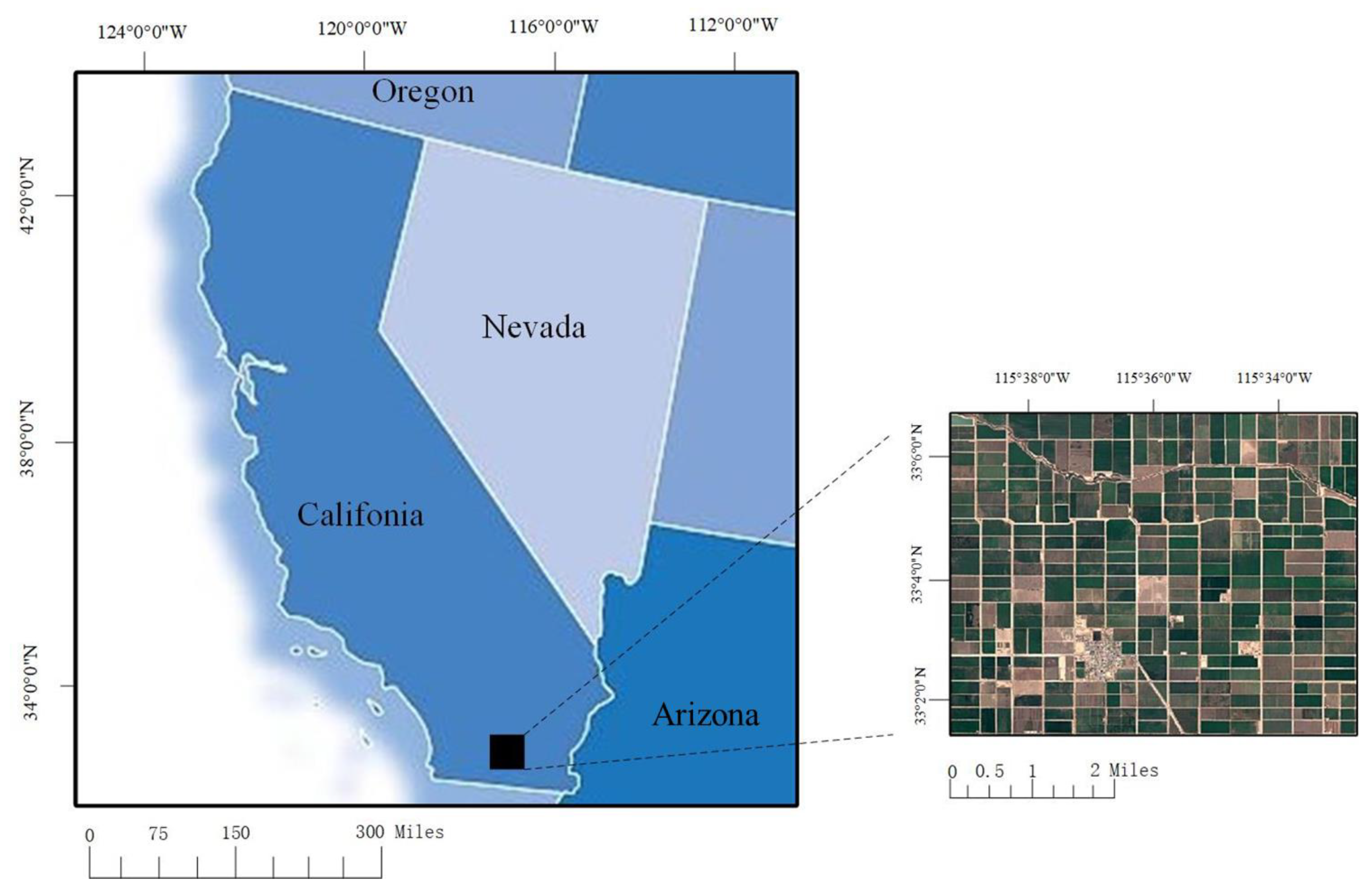
2.1. Study Area

California stands as the preeminent agricultural state in the United States, characterized by its highly advanced and predominantly irrigation-dependent farming systems. Agricultural land accounts for 30% of the state, and there are hundreds of agricultural and animal husbandry products. This indicates that the establishment of a crop mapping of California has profound significance. Thus, this study chose a certain area in California, as shown in Figure 1, as the study area.

The study area is situated in Imperial County, located in Southern California, with geographic coordinates of 33°07′8″ North latitude and 115°57′0″ West longitude. The area covers an area of about 12 km × 12 km, and the area perimeter is about 42 km. The area is located in the Colorado desert and low-altitude areas. The climate is a tropical desert climate, which is characterized by high annual average temperature, large annual temperature difference, greater daily temperature difference, and scarce precipitation. This area is one of the main producing areas of onions, sugar beets, and alfalfa in California. At the same time, the annual average temperature in this area is higher than 27 °C [35]. The annual rainfall is scarce, which is lower than the average annual rainfall in the United States. As a result, irrigation is the main method of crop water supply in this area. Six classes were selected for analysis: alfalfa, durum wheat, lettuce, sugar beets, onion, and other hay/non-alfalfa.

2.2. Data Collection and Pre-Processing

In this study, the temporal archived SPOT5 data were used in central Imperial County between 2007 and 2016. Image data that meet the research requirements of this article were sampled and analyzed. The data were collected and extracted from the downloaded SPOT5 satellite image data as experimental data. These data took 9 years to obtain different types of land cover use, and each remote sensing image was acquired in June of that year.

This paper adopts the Cropland Data Layer (CDL) of the United States Department of Agriculture (USDA) from 2007 to 2016 as the reference data for manual crop segmentation, and on this basis, experiments were carried out to verify the algorithm of this paper. CDL is regularly released by the USDA, covering 48 states in the United States [36]. Due to its wide coverage and long-term continuous data, including hundreds of different crop types, CDL data are widely used in various remote sensing crop research. However, the classification accuracy of the data is not particularly good, especially since there are some obvious errors, which need to be corrected by the researchers themselves according to the actual situation [37]. The misclassification of CDL in this study area is mainly concentrated at the junction of different types of features, so we visually corrected the error based on the CDL data and marked and plotted the labeled map data, as shown in Figure 2.

The process of drawing labeled classified images is to first resample the spatial resolution of the CDL obtained in the USDA to high resolution, and then overlay the remote sensing image downloaded by Google Earth on the CDL image to determine the boundaries of different types of crop farmland [38]. Secondly, the fields of the six main crops studied in this paper are manually delimited. In order to reduce the error caused by the marking process, a pixel is buffered inward from the field boundary when the image is marked. Finally, the same type of crop manually marked is merged into one class. Detailed information on the modification of labeled data is reported in

Table 1. Detailed information on the modification of labeled data.

Class	Number of Pixels
Alfalfa	123,925
Lettuce	9008
Sugar beets	18,632
Onions	15,374
Durum wheat	21,452
Other hay	24,395

.

This experiment is a crop classification task based on remote sensing images. The annotation of remote sensing image data for large-scale production time series is very time-consuming and laborious. There is a large remote-sensing image in the experiment. One part is selected for training, and the other part is tested. These images cannot be fully used for neural network training because the workstation cannot withstand memory and the size is different. Therefore, we first let them do random cutting, randomly generated x, y coordinates on the image, and then picked out the 256 × 256 small graphics in this coordinate. Therefore, based on the image of 2007, this study randomly selected 10% of each year from 2008 to 2016 as the training set, and the remaining data from 2008 to 2016 as the test set, in which the training set carried out data enhancement processing, such as brightness enhancement, rotation, etc. After preprocessing, 1000 images of the training set and 400 images of the test set were obtained. According to the needs of the neural network structure of this study, a square patch with a slice size of 256 × 256 was used as input in the data set. For the network with a multi-scale fusion structure, it is necessary to downsample the input of each 256 × 256 slice to 128 × 128 and input them into the neural network together. It should be noted that the training set and test set of the same year randomly selected in this study do not overlap.

3. Methods

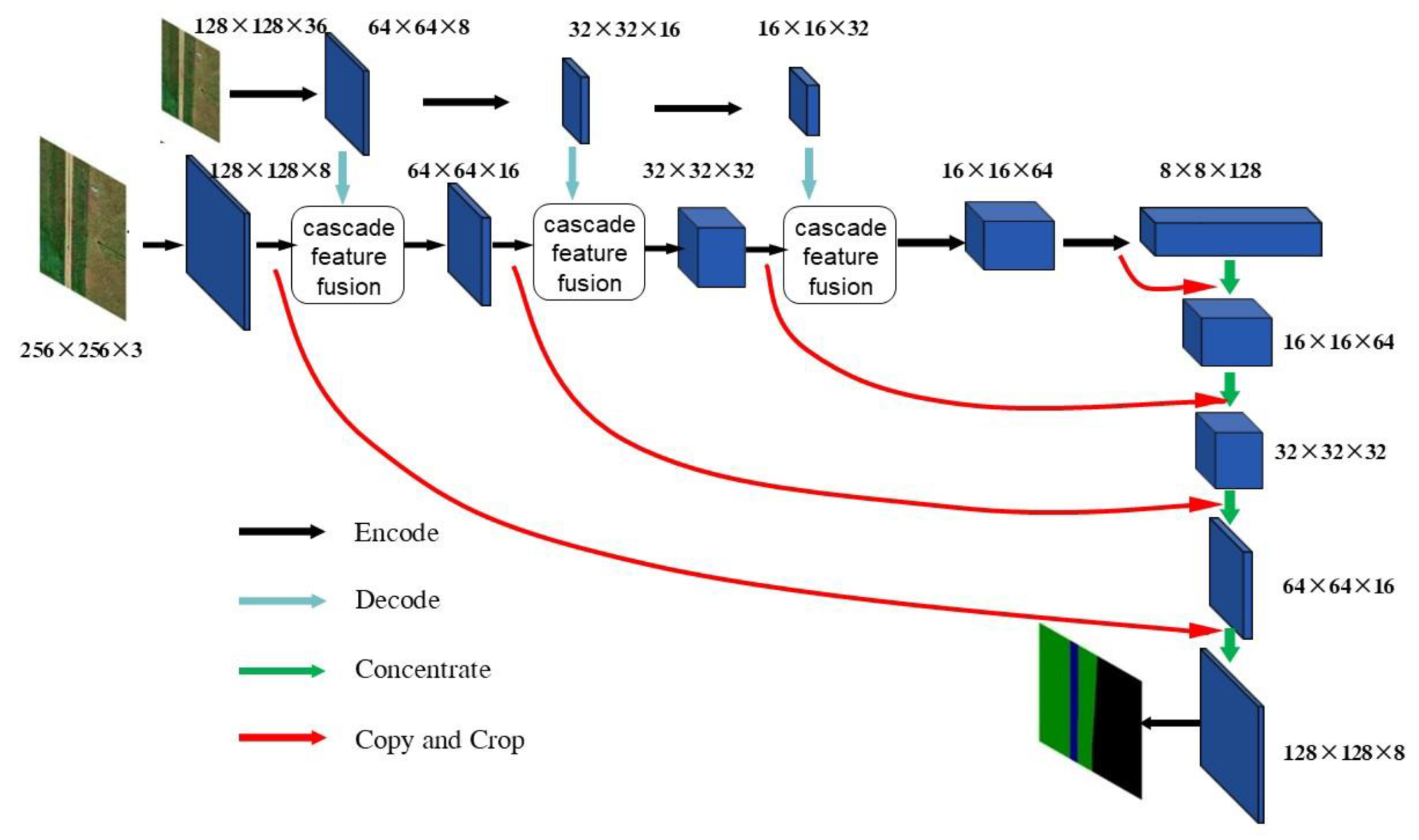
3.1. Multi-Scale Fusion Network Model (MSFNet)

The task of this paper is pixel-level semantic segmentation. As the first end-to-end semantic segmentation network, FCN has a disadvantage in that the details of the segmentation results are not good enough. Many researchers have made improvements on the basis of FCN and proposed many effective networks. Among them, the widely used semantic segmentation includes U-Net, PSPNet, and DeepLabv3+. Although PSPNet and DeepLabv3+ achieved the best results in many public datasets, the structure of U-Net is simple and standardized, and it has good performance on large images and complex medical images, and the effect on the few-shot datasets is more significant. Therefore, U-Net is more in line with the task requirements of this paper, and this paper improves on the basis of U-Net and proposes a semantic segmentation network MSFNet that pays more attention to multi-scale fusion.

3.1.1. Network Architecture Subsubsection

At present, the common semantic segmentation depth learning model mostly adopts the single-channel end-to-end network structure. The disadvantage of this single-channel network structure is that it is difficult to learn global and local features at the same time: If the size of the convolution kernel in the convolutional layer is reduced to reduce the receptive field, the learning of local texture details can be strengthened. However, some global characteristics will be ignored. Through the analysis of remote sensing image data, the feature distribution in remote sensing images is more complicated and changeable than traditional image data. In remote sensing images, not only a large number of features are gathered and distributed, but also a few or even a single vegetation or building are distributed in isolation among other features. Therefore, the deep learning model should comprehensively consider this different situation. The MIFNet model proposed by Zhang et al. has achieved good results in the semantic segmentation of pathological images using input data of different scales [39]. It is proved that the use of multi-resolution input can make the deep learning model have a good effect on learning global and local features. This paper absorbs its core ideas, combines the characteristics of remote sensing images, and proposes a multi-scale input MSFNet model, as shown in Figure 3, based on the U-Net model structure with good performance in the large image field.

On the basis of the U-Net, by increasing the input of low-scale images, the features of different scales of the image can be well extracted. The high-scale branches in the model can enhance the extraction of local features, and the low-scale branches can enhance the extraction of global features, so there is no need to worry about the loss of single-channel features. The MSFNet model can achieve the best results when using the data of two different resolutions of the original image, with a double-downsampled image as input. The downsampling method uses bilinear interpolation:

Knowing the value of $f(x)$ at the four points $V_{aa}=\left(x_a,y_a\right),V_{ab}=\left(x_a,y_b\right),V_{ba}=\left(x_b,y_a\right)$, and $V_{bb}=\left(x_b,y_b\right)$, we need to calculate the value of $f(x)$ at point $Z=(\mathrm{x},\mathrm{y})$. First, perform linear interpolation in the $x$ direction to obtain the following formula:

$$f\left(W_a\right)\approx {\displaystyle \frac{x_b-x}{x_b-x_a}}f\left(V_{aa}\right)+{\displaystyle \frac{x-x_a}{x_b-x_a}}f\left(V_{ba}\right) \mathrm{where} W_a=\left(x,y_a\right),$$

(1)

$$f\left(W_b\right)\approx {\displaystyle \frac{x_b-x}{x_b-x_a}}f\left(V_{ab}\right)+{\displaystyle \frac{x-x_a}{x_b-x_a}}f\left(V_{bb}\right) \mathrm{where} W_a=\left(x,y_b\right),$$

(2)

Then, linearly interpolate in the $y$ direction to obtain the following formula:

$$f(Z)\approx {\displaystyle \frac{y_b-y}{y_b-y_a}}f\left(W_a\right)+{\displaystyle \frac{y-y_a}{y_b-y_a}}f\left(W_b\right),$$

(3)

The final result of bilinear interpolation is as follows:

$$\begin{array}{l}f(x,y)\approx {\displaystyle \frac{f\left(V_{aa}\right)}{\left(x_b-x_a\right)\left(y_b-y_a\right)}}\left(x_b-x\right)\left(y_b-y\right)+{\displaystyle \frac{f\left(V_{ba}\right)}{\left(x_b-x_a\right)\left(y_b-y_a\right)}}\left(x-x_a\right)\left(y_b-y\right)\\ \hspace{1em}\hspace{1em}\hspace{1em}+{\displaystyle \frac{f\left(V_{ab}\right)}{\left(x_b-x_a\right)\left(y_b-y_a\right)}}\left(x_b-x\right)\left(y-y_a\right)+{\displaystyle \frac{f\left(V_{bb}\right)}{\left(x_b-x_a\right)\left(y_b-y_a\right)}}\left(x-x_a\right)\left(y-y_a\right)\end{array},$$

(4)

In the design of MSFNet, the model uses multi-scale input to extract features of different scales. Specifically, the model includes two input branches: a high-scale branch (256 × 256 resolution) and a low-scale branch (128 × 128 resolution). The 128 × 128 image is obtained by downsampling the 256 × 256 image. The high-scale branch focuses on extracting local detail features, while the low-scale branch enhances the capture of global features by down-sampling the input data. The data of each branch are processed by an encoder with the same structure to extract deep features, and feature fusion is performed at different levels of the network. The fused features are gradually restored to the original high resolution through the decoder to generate the segmentation results corresponding to the input image. Compared with the traditional U-Net model, MSFNet not only has a significant improvement in segmentation accuracy (especially in detail processing and global consistency) but also reduces the number of convolution kernels in high-scale branches and reduces the number of overall parameters, making the model more computationally efficient. Experiments show that while maintaining high segmentation accuracy, the parameters of MSFNet are much lower than those of the original U-Net model, which has obvious advantages in the semantic segmentation task of complex remote sensing images.

In the MSFNet model, the resolutions of the two input images are 256 × 256 and 128 × 128 pixels, respectively, and the 128 × 128 image is obtained by down-sampling the 256 × 256 image. The data from both resolutions are processed through identical encoder structures to generate deep feature maps. These features are then fused at various layers within the model. Subsequently, the decoder restores the data to the high-resolution input size, producing a prediction result that corresponds to the original input image. The down-sampling processing image makes the data lose some detailed features, but it can improve the model’s ability to learn global features. Since the encoder of the low-scale branches has a smaller parameter scale, more convolution kernels can be used to improve the model’s ability to learn data features. However, experiments show that the number of convolution kernels that do not need to reach the common U-Net model can achieve good results. In high-scale encoders, it is only necessary to use fewer convolution kernels to recover the details of the model lost in low-scale encoders and reduce the number of convolution kernels in high-scale encoders. The lost features can be supplemented with low-scale branches. By comparison, the MSFNet model obtains a higher segmentation accuracy than the ordinary U-Net model, and its parameters are much smaller than the U-Net model.

3.1.2. Cascade Feature Fusion

In the previous section, the neural network could consider global and local features at the same time by introducing low-scale branches. Since the scales of the feature maps obtained after the input data of different resolutions pass through the encoder are still different, they cannot be directly superimposed. In order to combine the feature images from different resolutions, the feature fusion structure shown in Figure 4 is designed. Feature fusion in MSFNet mainly uses a combination of high-scale and low-scale features so that the fusion result is used in the high-scale branches and transmitted to the decoder.

The large-scale image Input1 is first mapped nonlinearly by a convolution layer of 1×1 to improve the feature expression ability of the data and then standardized by batch normalization layers to prevent gradient explosion or disappearance. The maximum pool layer is used to obtain the feature map of the same scale as the Input2 for feature fusion. Input2 is processed by a convolution operation to obtain a global feature map, and then the same convolution and standardization processing as Input1. The size of Input1 and Input2 is unified, and two layers are superimposed. The superimposed feature maps are fused and output by a convolution operation. Finally, the size of the output feature graph is the same as that of Input1, and the number of channels is the sum of the number of channels of two input feature images. The fusion structure pays less attention to global features and pays more attention to local detail texture features.

In the process of cascade feature fusion, a 1 × 1 convolution operation is first per-formed on the large-scale input image Input1 to perform nonlinear mapping, thereby improving the feature expression ability. Then, the batch normalization layer is used to standardize the feature map to prevent the gradient from exploding or disappearing. Then, the size of the feature map is adjusted by the maximum pooling layer (max pooling) to make it the same size as the feature map of the small-scale input image Input2, which is convenient for subsequent feature fusion. For Input2, the global feature map is first obtained by convolution operation, and then convolution and standardization are per-formed as in Input1. After the size of the two input feature maps is unified, the superposition operation is performed. The superimposed feature maps are further fused by a convolution operation. The final output feature map size is consistent with Input1, and the number of channels is the sum of the number of channels of the two input feature maps. This fusion mechanism can not only effectively combine high- and low-scale features, but also further strengthen the expression of local detail features. By gradually transferring global features to local features of high-scale branches, the model can retain global semantic information and enhance the ability to capture local details. This process significantly improves the segmentation accuracy of the model, especially in complex scenes. Compared with the traditional U-Net, MSFNet not only improves the segmentation performance but also greatly reduces the number of parameters of the model, making it perform better in scenarios with limited computing resources.

3.2. PSML Model

3.2.1. Model-Agnostic Meta-Learning (MAML)

The purpose of MAML is to obtain the optimal initial parameters through iterative training. Moreover, iterative training refers to multi-level iterative training of different tasks under the same task distribution. The purpose is to learn the similarities and differences between different tasks so as to achieve fast adaptation to new tasks. The selection of related tasks means that the inner loop of MAML randomly extracts the training set according to a specific number each time. By obtaining new initial parameters, the model can converge faster.

Assume there are three related tasks: T1, T2, and T3. Firstly, randomly set the initial parameter $\theta$ of the neural network. For task T1, the neural network first receives training data and then generates a loss. Based on the loss, T1 is minimized using stochastic gradient descent or other gradient descent methods. Obtain optimized model parameters ${\theta }_1^{\prime }$ through iterative training steps. Similarly, tasks T2 and T3 obtain optimal parameters ${\theta }_2^{\prime }$ and ${\theta }_3^{\prime }$ in the same way. The optimal parameters for different tasks are shown in Figure 5.

Assuming the model is $f_{\theta }$, which can be described by the parameter $\theta$, the distribution probability of the task is defined as P(T). Firstly, initialize the parameter $\theta$ randomly with a random value, and then the tasks T_i in the task set are adopted through the probability distribution P(T). For each task T_i, calculate the loss function $L_{T_i}\left(f_{\theta }\right)$ for each task, minimize the loss function through gradient descent, and find the parameters that can minimize the loss function; the process is as follows:

$${\theta }_{\mathrm{i}}^{\prime }=\theta -\alpha {\nabla }_{\theta }{L}_{T_i}\left(f_{\theta }\right),$$

(5)

where ${\theta }_i^{\prime }$ is the optimal parameter for a task T_i, $\theta$ is the initial parameter, $\alpha$ is the hyperparameter, and ${\nabla }_{\theta }{L}_{T_i}(f_{\theta })$ is the gradient of a task T_i.

More concretely, the updating is as follows:

$$\underset{\theta }{\min }{\displaystyle \sum _{{\mathcal{T}}_i~p(\mathcal{T})}{\mathcal{L}}_{{\mathcal{T}}_i}}\left(f_{{\theta }_i^{\prime }}\right)={\displaystyle \sum _{{\mathcal{T}}_i~p(\mathcal{T})}{\mathcal{L}}_{{\mathcal{T}}_i}}\left(f_{\theta -\alpha {\nabla }_{\theta }{\mathcal{L}}_{T_i}\left(f_{\theta }\right)}\right),$$

(6)

Similarly, each task obtains different update parameters by updating the initial parameters, thereby obtaining the relatively optimal parameter set for each task:

$${\theta }^{\prime }=\left\{\left.{\theta }_1^{\prime },{\theta }_2^{\prime },{\theta }_3^{\prime }\right\}\right.,$$

(7)

Before sampling the next update task, a meta-update or meta-optimization strategy is used. In the previous step, the relatively optimal parameters ${\theta }_i^{\prime }$ were calculated through gradient descent, and the initialized random parameter $\theta$ was updated based on the gradients corresponding to the parameters in the task T_i. This moved the initial random parameter $\theta$ to a relatively optimal position. In the training of a batch of tasks, the number of steps in gradient descent is reduced, which is called meta updating. The update process is as follows:

$$\theta =\theta -\beta {\nabla }_{\theta }{\displaystyle \sum _{T_i~p\left(T\right)}^{ }{L}_{T_i}\left(f_{{\theta }_i^{\prime }}\right)},$$

(8)

where $\theta$ is the initial parameter, $\beta$ is the hyperparameter, and ${\nabla }_{\theta }{\displaystyle \sum _{T_i~p\left(T\right)}^{ }}{L}_{T_i}\left(f_{{\theta }_i^{\prime }}\right)$ represents the gradient result of task T_i calculated through parameter ${\theta }_i^{\prime }$.

Figure 6 shows the process of MAML, and the training process can be divided into inner and outer loops.

3.2.2. Particle Swarm Optimization to Optimize MAML

Particle swarm optimization (PSO) is a swarm intelligence algorithm [40]. In this paper, PSO is used to optimize the learning rate of the inner and outer loop of MAML, so PSML is used to represent the MAML after PSO optimization. Firstly, set the maximum number of iterations in the search space, the number of independent variables in the objective function, and the maximum velocity and position information of particles. Next, initialize the velocity and position in the velocity space and search space, and set the particle swarm to randomly initialize the flight velocity M. Next, the fitness function is defined, where the individual extremum is the global optimal solution obtained by each particle from the optimal solution. The update process of speed and position is as follows:

$$V_{id}=\omega V_{id}+C_{1}random\left(0,1\right)\left(P_{id}-X_{id}\right)+C_{2}random\left(0,1\right)\left(P_{gd}-X_{id}\right),$$

(9)

$$X_{id}=X_{id}+V_{id},$$

(10)

where $\omega$ is the inertial coefficient, $C_1=C_2\in [0,4]$ is the acceleration coefficient. $random\left(0,1\right)$ is a random number in the 0 to 1 interval. $P_{id}$ and $P_{gd}$ represent the individual optimal position and global optimal value found by the particle, respectively.

This paper uses the PSO algorithm to optimize the MAML learning rate, accelerate model convergence speed, and improve model performance. The simplified description function is as follows:

$$\min f\left(r_1,r_2\right)=\min L\left(f_{\theta }\right)$$

(11)

where $r_1$ and $r_2$ are the learning rates of the inner loop and outer loop in MAML, respectively.

3.2.3. The Fusion of MAML and MSFNet

MAML has good generalization ability and can improve model training speed by quickly learning initial parameters. This article is based on the MSFNet network of MAML to improve model generalization and reduce neural network training time. The proposed method is designed for the classification task of semantic segmentation, and the loss function of its neural network is as follows [41]:

$$L_{T_i}\left(f_{\theta }\right)={\displaystyle \sum _{x_j,y_j~T_i}^{ }{y}_i\log f_{\theta }\left(x_j\right)+} \left(1-y_j\right)\log \left(1-f_{\theta }\left(x_j\right)\right),$$

(12)

The detailed process of applying MSFNet to MAML is as follows:

(a)

Assume there exists a parameterized model $f_{\theta }$ consisting of parameter $\theta$ a and the distribution $P\left(T\right)$ on the task. Firstly, randomly initialize the model parameter $\theta$;

(b)

Some different batches of tasks ${\mathrm{T}}_{\mathrm{i}}$ are randomly selected from task $T$, that is, $T_i~P\left(T\right)$. For example, there are three selected tasks: $T=\left\{T_1\right.,T_2,\left.T_3\right\}$;

(c)

Inner loop: For each task ${\mathrm{T}}_{\mathrm{i}}$ taken from $\mathrm{T}$, sample $\mathrm{k}$ data points and prepare training and testing datasets:

$$D_i^{train}=\left(x_1,y_1\right)\dots \left(x_k,y_k\right),D_i^{test}=\left(x_1,y_1\right)\dots \left(x_k,y_k\right)$$

(13)

The neural network first receives training data $D_{train}$ and then generates a loss, minimizing the loss using stochastic gradient descent or other gradient descent methods. Obtain the optimized model parameter ${\theta }_i^{\prime }$ through iterative training steps. Similarly, other tasks obtain optimal parameters in the same way.

(d)

Outer loop: The meta-test set $D_{test}$ is utilized to minimize the loss function based on the parameters obtained from the inner loop. This process aims to derive an optimal set of initialization parameters $\theta$, which enhance the model’s ability to quickly adapt to new tasks.

The process iterates through steps (b) to (d) for n cycles, the detailed diagram of MAML in MSFNet is shown in Figure 7.

3.3. Experimental Setup

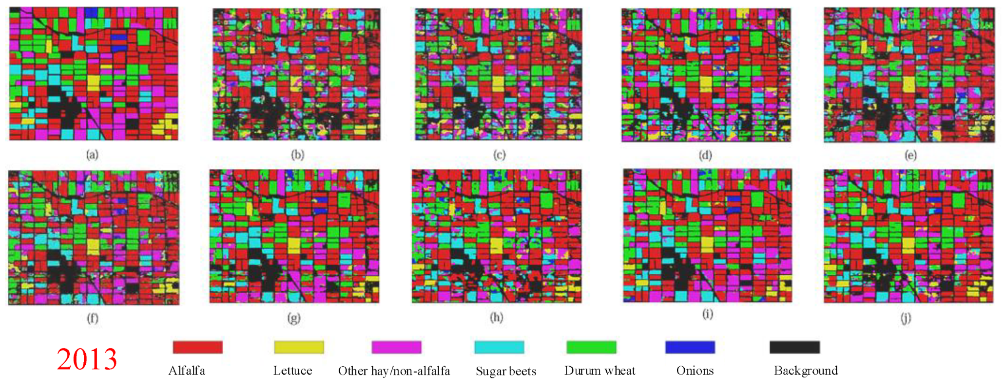
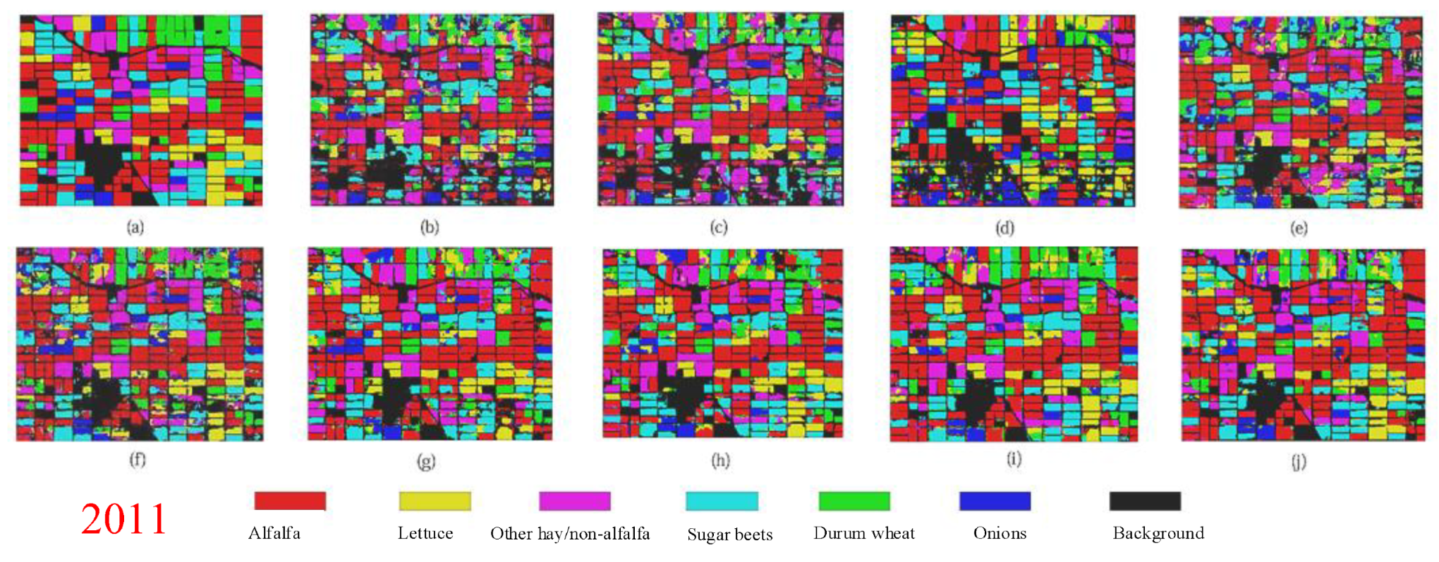
In terms of parameter settings for U-Net network training, the initial training step was set to 0.0001 [42,43,44], and Adam was applied as the optimizer. The experimental results showed that 0.0001 can ensure stable convergence in remote sensing image segmentation tasks and achieve the best segmentation accuracy on the validation set. The experiment set the meta-training step for the inner and outer loop learning rates of MAML to 0.0001, set the training step to 0.001 [45,46], set the convolution core size of the U-Net network to 3 × 3, and set the convolution layer outputs to 32, 32, 64, 64, 128, 64, 64, 32, and 7. It should be noted that the training image is an RGB image, so the input layer is three layers. As it is a seven -class classification task, the output layer is seven layers, and other parameters are set by default. The average accuracy (AA), F1-score, and mean IoU (mIoU) were used as the criteria for evaluating model performance.

The U-Net model, Deep Labv3 + model, and PSPNet model were compared with the MSFNet model proposed in this paper and the MSFNet model optimized by PSO and MAML. Among them, the U-Net model is a classic semantic segmentation network, and the DeepLabv3+ model and the PSPNet model are two deep learning models with better semantic segmentation effects proposed in recent years. In addition, the U-Net model uses the encoder–decoder structure, and the PSPNet uses the spatial pyramid pooling structure. To explore the effectiveness of the PSO algorithm, the MAML network optimized by the bat algorithm (BAML) was used as a comparison test. The experimental equipment is a Z7-CT5 NS workstation, the operating system is Windows 10, the TensorFlow machine learning platform is used, and the NVIDIA GeForce GTX1660 Ti GPU is equipped.

4. Results

We evaluated the performance of MSFNet and PSML and compared them with U-Net, PSPNet, and Deep Labv3+. The MAML approach divides the training process into internal and external phases. Correspondingly, our dataset was split into a training set and a meta-training set. The internal loop utilized the first dataset to develop the model’s fundamental ability to handle each task. External training used the second data set, focusing on enhancing the generalization ability of the model across multiple tasks. During the experiment, we simultaneously input the training set into both the inner and outer loops. This approach allows the model to effectively develop both task-specific proficiency and broad generalization capabilities, resulting in optimal test accuracy. Subsequently, we employed a prepared test dataset to evaluate the accuracy of the trained model. The test results are visually represented in Figure 8, Figure 9, Figure 10, Figure 11, Figure 12, Figure 13, Figure 14, Figure 15 and Figure 16.

From the experimental results, it can be seen that the MSFNet with PSML had the highest test accuracy. Obviously, for competitive methods such as U-Net, PSPNet, and DeepLabv3+, there was a large amount of speckle noise in the classification result image, resulting in low crop mapping accuracy. Specifically, when dealing with large-scale remote sensing images, the U-Net structure is prone to insufficient capture of global features due to the lack of multi-scale feature fusion, resulting in a large amount of speckle noise in the generated classified images. PSPNet and DeepLabv3+ enhance the extraction ability of global features by introducing modules such as pyramid pooling. On the data set of this study, although they can capture certain global features, they still have detail loss and inaccurate classification when dealing with remote sensing images with rich details. The MSFNet proposed in this paper captures local detail information in the high-resolution branch and captures global features in the low-resolution branch through the design of multi-scale input. Through the effective fusion of multi-scale features, MSFNet can significantly reduce the noise in the classification results and better preserve the boundary details, making the classification map more accurate. This advantage is reflected in

Table 2. Results of the study area.

Method	Alfalfa	Other Hay	Durum Wheat	Lettuce	Onions	Sugar Beets	Back-Ground	AA	F1_Score	mIoU
U-Net	92.096%	81.883%	82.279%	88.165%	86.158%	89.191%	89.044%	87.675%	81.992%	77.254%
PSPNet	89.136%	81.600%	88.878%	86.062%	87.196%	87.692%	92.295%	87.960%	85.343%	78.502%
DeepLabv3+	91.752%	90.453%	81.456%	89.612%	86.951%	90.586%	90.761%	88.795%	87.398%	80.045%
MSFNet	92.429%	87.475%	83.634%	88.584%	88.174%	91.108%	90.144%	89.359%	88.835%	81.130%
MAML+ U-Net	93.164%	89.162%	83.946%	90.432%	87.967%	94.852%	91.364%	90.126%	88.357%	79.521%
PSML+ U-Net	93.843%	90.912%	87.691%	92.867%	93.458%	91.475%	91.654%	91.700%	89.156%	85.943%
MAML + MSFNet	94.216%	94.363%	87.417%	93.649%	94.074%	97.337%	93.194%	93.705%	88.699%	87.699%
BAML + MSFNet	96.193%	92.764%	92.584%	93.895%	95.716%	95.146%	93.254%	94.221%	89.638%	88.167%
PSML + MSFNet	98.936%	88.743%	91.701%	94.879%	94.872%	94.919%	96.891%	94.902%	91.901%	90.557%

, and the overall classification accuracy of MSFNet was still high, reaching 89.359%. It is worth noting that the mIoU of MSFNet was 3.876%, 2.628%, and 1.085% higher than that of U-Net, PSPNet, and DeepLabv3+, respectively, indicating that the multi-scale fusion structure had greater improvement in crop classification of large-scale remote sensing images than the structure with only a single input channel.

In order to further improve the generalization ability of the model on complex tasks, this paper used the MAML (Model-Agnostic Meta-Learning) algorithm to divide the training process into an inner loop and outer loop, which were then used to learn the basic ability of the task and improve the generalization performance of the model. In this way, MSFNet can not only achieve high segmentation accuracy on specific tasks but also show strong generalization ability. In our experiment, the average accuracy of MSFNet optimized by MAML was 4.346% higher than that of the unoptimized model, which further verifies the effectiveness of MAML in complex remote sensing image segmentation tasks.

In this paper, the bat algorithm, which has recently shown better results, was chosen for comparison. The bat algorithm is also a swarm intelligence algorithm, which is widely used in deep learning [47]. The bat algorithm is inspired by the bat’s echolocation predation behavior. In terms of results, the bat algorithm introduces frequency to control the flight speed, resulting in a flight that is not as good as the randomness of particle swarms and more likely to fall into local optima but converges faster. The algorithm converges extremely fast and has better local search capability, but its global search capability is insufficient and it is prone to fall into local optimum, and its convergence speed becomes slower and slower as the bats become more and more concentrated in the later stages of the algorithm [48]. This paper further introduced the PSML (meta-learning based on particle swarm optimization) algorithm to improve the training effect of the model by optimizing the learning rate of the inner loop and the outer loop. Compared with traditional MAML, PSML can better balance the learning speed of internal and external loops, thus improving the generalization ability of the model. The experimental results showed that the MSFNet optimized by PSML was 0.681%, 2.263%, and 2.390% higher than the MSFNet optimized by BAML (meta-learning based on bat algorithm) in AA value, F1-score value, and mIoU value, respectively. This shows that the particle swarm optimization algorithm is superior to the bat algorithm in the global optimal search ability, and can better improve the adaptability of the model to different tasks, especially in the segmentation task of remote sensing image complex scene, showing strong generalization ability.

5. Discussion

5.1. Analysis of Factors Influencing the Changes of Crop Area

According to the results of the experiment, the crop maps of consecutive years from 2007 to 2016 were finally obtained. As shown in Figure 17, crops in the study area include durum wheat, alfalfa, sugar beets, onions, lettuce, and other hay/non-alfalfa. Among them, the planting area of alfalfa accounts for the largest proportion, far exceeding other crops, and showing an overall upward trend. The planting area of durum wheat is second only to alfalfa, showing an upward trend and then a downward trend, but it is still within a controllable range. Sugar beets, onions, lettuce, and other hay/non-alfalfa accounted for a relatively small proportion. The planting area of sugar beets showed an upward trend, and the other three types all oscillated within a certain range. As shown in Figure 18, the value of durum wheat and alfalfa fluctuated greatly, and the value of both was much higher than other crops in the study area. The value of sugar beets, onions, and lettuce was relatively low and fluctuates in a very small range [49,50].

The main factors affecting plant growth are moisture, air, light, soil conditions, and microorganisms. In addition, the growth environment requirements of different crops are different, or even quite different.

Durum wheat is an annual plant, usually planted in spring and harvested in autumn. Although the production of durum wheat is low, it is the second-largest wheat variety in the world, and the demand for durum wheat is increasing worldwide. Alfalfa is a perennial plant. California, Idaho, and Montana are the main growing states of alfalfa. Alfalfa has a well-developed root system, and the main root usually grows 2 to 3 m, so it is extremely resistant to drought. In southern California, there is plenty of sunshine, suitable for alfalfa growth; here, alfalfa can be harvested up to 12 times a year. Sugar beets have higher requirements for sunlight, temperature, rainfall, soil, and wind. Soft soil and low wind speed are conducive to the growth of sugar beet roots, and fertile soil is conducive to the accumulation of sugar. Although California is not the state with the largest area of sugar beets cultivation, Imperial has benefited from high local sunshine intensity and advanced irrigated agriculture and has achieved a yield of about 160 tons per hectare, reaching the world’s leading level. Moreover, California has a long history of sugar beet. The first sugar beet factory in the United States is located in California. Onions and lettuce are common vegetables in American daily life. The root system of onion is concentrated in the topsoil layer, and the drought resistance is weak. It is sensitive to sunshine length, temperature, and precipitation, and has certain requirements for soil. The root system of onions is shallow and does not require much water, while sandy soil is conducive to the drainage of water. Lettuce has a large leaf area and a large amount of water evaporation, so lettuce is sensitive to sunlight and water. High-intensity sunlight is bad for the growth of lettuce.

Taking five crops of durum wheat, alfalfa, beet, onion, and lettuce as the objects, combined with the characteristics of different plants and the natural factors affecting plant growth, the changes of crop planting area in the study area were analyzed, and the main planting decision-making factors were discussed. Seventeen available meteorological data were analyzed, including air pressure, temperature, precipitation, surface temperature, dew point temperature, relative humidity, evaporation, potential evaporation, total wind speed, north wind speed, east wind speed, cloud cover, net sunshine intensity, total sunshine intensity, sunshine hours, ultraviolet intensity, surface runoff. SPSS software was used for statistical analysis to explore the most important influencing factors. Durum wheat occupies a pivotal position in American food culture, as the main food crop is affected by national policies. Facts have proved that the analysis of all factors of meteorological conditions does not show an obvious correlation.

Alfalfa is sunny and grows rapidly in sunny places, which is suitable for large-scale planting in sunny places. As an important feed crop, alfalfa has a huge market demand. California has a warm climate all year round and well-developed irrigated agriculture is very suitable for the growth of alfalfa. Moreover, alfalfa has strong drought tolerance, which is particularly important today when water resources are insufficient. As shown in Figure 19a, the annual average relative humidity in Imperial varies within a limited range. From 2013 to 2014, California experienced dry weather, with a significant decrease in precipitation and corresponding changes in air humidity. According to SPSS software analysis, the relative humidity in the meteorological data had the highest correlation with the planting area of alfalfa, and the Pearson Correlation Coefficient was 0.512. This shows that there is no significant correlation between the change in alfalfa planting area and the change in meteorological conditions. Because alfalfa produces harmful substances to the soil during its growth, it needs regular crop rotation, which is the main factor that affects planting decisions.

As an important economic crop, sugar is the main economic value of sugar beets. The influence of climatic conditions on sugar beets includes two parts: one part is the growth of the root system and the other part is the accumulation of sugar. Extended periods of sunshine coupled with significant diurnal temperature variations create optimal conditions for sugar accumulation in plants. As shown in Figure 19b, the cloud cover in Imperial showed a trend of extremely slow growth, which remained unchanged for many years. Sugar beet requires long sunshine but not strong, California strong sunshine intensity is not conducive to sugar beet growth. Therefore, clouds help reduce the intensity of sunlight and keep the duration of sunlight unchanged. According to the analysis of SPSS software, the correlation between cloud cover and sugar beet planting area in meteorological data was the highest, with a Pearson Correlation Coefficient of 0.783, a two-tailed significance test of 0.007, and a statistically significant correlation of 0.01 level. Therefore, under high-intensity sunlight conditions, cloud cover is the main factor affecting sugar beet planting decisions in meteorological data.

The well-developed irrigated agriculture in California made up for the lack of rainfall. As shown in Figure 19c, surface runoff presents fluctuations within a certain range. The onions are concentrated in the topsoil layer, which does not require much water, and excessive ground runoff will cause hypoxia in the root system, which is not conducive to the growth of onions. According to SPSS software analysis, the correlation between surface runoff and onion was the highest in meteorological data, and the Pearson Correlation Coefficient was −0.535. This means that ground runoff and onion planting area are generally negatively correlated, that is, ground runoff has a negative impact on onions. This is consistent with our analysis conclusion. Affected by the unique status of onions in American food culture, planting decisions are affected by many factors, so the correlation is low when only climatic conditions are analyzed.

Lettuce is a shade-loving plant, that does not require high light intensity, and strong light will burn its leaves. Therefore, light is the main factor affecting the growth of lettuce. As shown in Figure 19d, the total sunshine intensity in Imperial has been at a high level for many years and declined in a small range from 2007 to 2016. According to the analysis of SPSS software, the correlation between total sunshine intensity and onions in meteorological data was the highest; the Pearson Correlation Coefficient was −0.945, the two-tailed significance test was 0, and the statistical significance had a significant correlation level of 0.01. This means that there is a significant negative correlation between the total sunshine intensity and the planting area of lettuce. This is consistent with our analysis and conclusions suggesting that the total sunshine intensity is the main factor that affects lettuce planting decisions.

For the crops in the study area, the changes in the planting area were not only affected by natural conditions but also by economic values and national policies. The research survey shows that during the period from 2000 to 2012, the overall population of dairy cows in California showed an increasing trend. With the increase in the size of the dairy herd, the greenhouse gas emissions from dairy manure management and intestinal fermentation also showed a similar trend [51]. Alfalfa is the main feed for dairy cows. As shown in Figure 17, its planting area showed an increasing trend from 2007 to 2016, and the corresponding carbon emissions continued to rise. However, since 2000, California has been affected by long-term emission reduction trends. As shown in Figure 19, from 2007 to 2016, California’s crop planting area has been decreasing. By 2020, carbon emissions from crop production accounted for 21% of agricultural carbon emissions [51]. Carbon emissions from planting and harvesting crops have generally declined.

The direct carbon emissions caused by cultivated land use in this region mainly come from agricultural machinery energy consumption, biological respiration, soil organic matter decomposition, fertilizer application, etc. [15]. The calculation formula for regional direct carbon emissions is as follows:

$$E_k=A_i\times {\delta }_i$$

(14)

where $E_k$ represents the direct carbon emissions (measured in kilograms), i denotes the specific land use type, $A_i$ signifies the area of land use type i (measured in square meters), and ${\delta }_i$ represents the carbon emission (or absorption) coefficient specific to land use type i.

As shown in Figure 20, we calculated the total cultivated area in the region by summing the areas of alfalfa, durum wheat, other hay/non-alfalfa, onions, canola, and lettuce. As shown in Figure 21, using the average carbon emission coefficient for cultivated land of 0.0422 kg/m² [52], we then derived the total carbon emissions from cultivated land in the area. Since the area’s cultivated land in 2007 significantly differed from other years (the total carbon emissions in 2007 were nearly twice the average of the total emissions from 2007 to 2016), it was not possible to accurately reflect the trend in total carbon emissions for the region. Therefore, we considered the changes in total carbon emissions from 2008 to 2016 to predict the total carbon emissions for the region, noting a year-by-year decrease in total carbon emissions from cultivated land as the years progressed. The abovementioned analysis shows that the method proposed in this paper accurately reflects the change in crop planting area in Southern California and is expected to provide technical support for regional carbon neutrality.

5.2. Prediction Analysis of Crop Planting Area Change

In order to achieve the purpose of guiding the optimization of the planting structure in the region, we use the price, relative humidity, cloud cover change, surface runoff, sunshine intensity, policy, characteristics, classification of importance discussed in the previous part as characteristics to predict the change in crop planting area in the region.

We divided the policy impact into three levels: high (2), medium (1), and low (0.5). According to the research and investigation, from 2007 to 2016, alfalfa was more affected by relevant policies, such as the increase in the number of cows (alfalfa is the main feed for dairy cows), low-carbon emission reduction, and other policies. As the main food crop, durum wheat is affected by relevant policies, and the planting area fluctuates greatly during this period. We ranked it as highly affected by policies. Sugar beet and onion are less affected by relevant policies, and the proportion of planting area is general. We ranked them as medium affected by policies. Lettuce is less affected by relevant policies, and the planting area is low. We classified it as low affected by policies [49].

We divided the adaptability of crops to the environment into three levels: high (2), medium (1), and low (0.5). Hard wheat has good cold resistance, can grow on a variety of soil types, and has strong adaptability to the growth environment. We classified its adaptability to the environment as high. Alfalfa is a perennial herb that can grow under drought conditions, has strong adaptability to soil texture, and has good drought tolerance. We graded its adaptability to the environment as high. Sugar beet has strong adaptability to soil and can grow in a variety of soil types. It needs enough water to ensure the accumulation of yield and sugar. The demand for water is in the middle, and we ranked its adaptability to the environment as medium. Onions have relatively low requirements for the growth environment and can grow under various soil conditions, but they need good drainage conditions. We graded their adaptability to the environment as medium. Lettuce needs a mild climate and sufficient water to ensure growth, is sensitive to high temperatures and drought, and grows well in a cool and humid environment. We rated its adaptability to the environment as low.

We divided the importance of crops in the region into seven grades: PB (Area: over 6000), PM (Area: 6000~4000), PS (Area: 4000~2000), M (Area: 2000~1000), NB (Area: 1000~500), NM (Area: 500~250), and NS (Area: 250 below), and assigned the seven grades to 8, 4, 2, 1, 0.5, 0.25, 0.125, respectively. For example, from 2007 to 2016, the average planting area of alfalfa in this area was more than 6000, so we set the importance grade of alfalfa in this region as PB. Similarly, the average planting area of lettuce in this region was between 500 and 250, so we set the importance grade of lettuce in this region as NM.

During the model training process, we used the Random Forest Regressor model to complete the prediction of the planting area in the region. Firstly, in order to eliminate the difference in magnitude between different types of data, we normalized eight feature data. Then, we divide the data set into a training set and test set according to the ratio of 8:2 and set the random seed to 42 to ensure the repeatability of data splitting. The initial model evaluation index MSE value was 341,489.54, the RMSE value was 584.37, and the R² value was 0.96. Secondly, we improved the performance of the model by adjusting the hyperparameters through the GridSearchCV optimization model. The functional relationship between the training MSE loss value and the number of trees in the model is shown in Figure 22. During the training process, the MSE value of the model evaluation index was 50,694.67, the RMSE value was 225.15, and the R² value was 0.99. During the test process, the MSE value of the model evaluation index was 341,489.54, the RMSE value was 584.37, and the R² value was 0.96. As the number of trees increased, the MSE loss value gradually stabilized.

5.3. The Advantages and Disadvantages of the Model

Image segmentation of long time series is a very challenging task, especially for large-scale remote-sensing images. Due to the complex and changeable features of ground objects, the classification effect is greatly affected [53]. In this paper, a multi-scale fusion structure of MSFNet is proposed to solve the problem of different sizes of features in remote sensing images. Through the input of large-scale and small-scale images into the neural network for training, the extraction of global and local features has a better recognition effect for complex crops (such as sugar beets). The overall accuracy of MSFNet was improved by about 2% compared with the average accuracy of U-Net. For the difficulty of remote sensing image annotation, this paper introduced MAML to solve this problem. MAML divides the training process into an inner loop and an outer loop. The outer loop is responsible for updating network parameters, and the inner loop is responsible for fast learning to obtain better initial parameters. Through the introduction of the inner loop process, the purpose of rapid learning and increasing network generalization can be achieved. For the remote sensing images of different time series in this study, MAML can also achieve the characteristics of rapid learning of new tasks through its good generalization. The specific method is to use a small number of samples for fine-tuning training to achieve better results. Compared with the unoptimized network, the average accuracy of MAML-optimized MSFNet increased by about 4%, which proves that the introduction of MAML has better adaptability to remote sensing image tasks of different time series. In this paper, PSO was used to further optimize MAML, and the accuracy improved by about 1%.

Although the MSFNet proposed in this paper effectively solves the problem of global and local feature extraction in remote sensing images through multi-scale fusion structure and further improves the generalization ability of the model through MAML, we also found the limitations and potential error sources of the model during the experiment. The following section analyzes these problems in depth and proposes the improvement direction of future research.

The verification accuracy of this study is based on the assumption that the label data are 100% accurate. However, the label data in remote sensing images often rely on manual labeling, and the CDL dataset used in this paper especially relies on feedback from local farmers, which may introduce human error or delay feedback. Annotation errors in data may lead to low performance of the model in the training and testing stages, which reduces the generalization ability and final segmentation accuracy of the model. In order to reduce the impact of labeling errors on model performance, future research can consider introducing more automated labeling methods, such as combining UAV remote sensing data, using computer vision technology to assist labeling, or using higher resolution remote sensing data. This study used annual remote sensing data sets. The time series data in remote sensing images will be affected by factors such as rotation and seasonal changes, which may lead to fluctuations in classification accuracy. Future research can introduce multi-source remote sensing data (such as multi-spectral, Lidar, or hyperspectral data), which can provide more abundant crop spectral information and help to distinguish crops with similar characteristics. In addition, using time series models (such as LSTM or Transformer) to process time series data may help to capture dynamic changes in remote sensing images, thereby improving the generalization ability of the model for long-term sequence data. Although the introduction of MAML for meta-learning optimization makes the model better able to handle new tasks, the inner and outer loop learning rate settings of MAML still need to be manually adjusted during the experiment, which limits the model’s rapid adaptability to different tasks. Improper setting of the learning rate may lead to a decrease in the performance of the model on certain tasks and affect its overall generalization ability. In addition, although the PSO optimization algorithm has achieved a certain optimization effect on the adjustment of the learning rate, there is still a risk of falling into the local optimal solution due to the limited global search ability of PSO. Future research can continue to optimize the learning rate adjustment method of the MAML algorithm and explore more efficient meta-learning algorithms, such as automatic parameter adjustment methods or bionic intelligent algorithms, to further improve the generalization ability of the model. In addition, future experiments can carry out multi-task learning or transfer learning for different task scenarios so that the model can learn more shared features from different tasks, thereby improving its adaptability in different scenarios.

5.4. Contribution to UAV Remote Sensing

Subsequent research can quickly obtain high-resolution image data of different heights and angles through UAV remote sensing technology. UAV remote sensing technology not only provides flexible and efficient data acquisition methods but also significantly reduces costs and reduces manual intervention. Combined with the multi-scale fusion network (MSFNet) model proposed in this study, these high-resolution image data can significantly improve the accuracy and coverage of agricultural monitoring. Specifically, the multi-scale image data collected by the UAV are input into the MSFNet model after preprocessing to capture the multi-level features from the whole to the local. The feature fusion technology fuses the image features of different scales to enhance the accuracy and robustness of the model. Combined with the model diagnostic meta-learning (MAML) method, the generalization ability of the MSFNet model in different agricultural scenarios is improved, while the particle swarm optimization (PSO) algorithm optimizes the parameter update process of the neural network and avoids the local optimal problem. Through the comparative analysis of multi-temporal high-resolution remote sensing image data, the MSFNet model can carry out spatio-temporal dynamic analysis, timely detect the changing trend and abnormal situations in farmland, and take effective intervention measures to reduce the risk of agricultural production. This combination method not only improves the efficiency and accuracy of agricultural production but also provides strong technical support for the intelligent and accurate management of modern agriculture, which helps to optimize the planting structure and achieve sustainable agricultural development.

In the future, we will abide by relevant ethics, laws, and regulations in UAV remote sensing research. When using drones for agricultural monitoring, we strictly follow data privacy protection laws to ensure that data col-lection is limited to agricultural uses and to avoid obtaining irrelevant private information. In addition, the project complies with relevant Chinese and international UAV flight regulations, including flight altitude, airspace restrictions, and operating licenses, to ensure legal compliance. No violations of environmental or community rights were involved in the study.

6. Conclusions

In this study, an innovative multi-scale fusion network MSFNet was proposed by using the high-resolution remote sensing images of time series from 2007 to 2016 provided by SPOT5. Combined with the PSML (particle swarm optimization meta-learning) algorithm, the performance of the model in complex remote sensing tasks was significantly improved. Through multi-scale input, MSFNet solved the problem of insufficient global and local feature capture when dealing with large-scale remote sensing images by using traditional single-scale networks. PSML optimized the training process of the model and enhanced the generalization ability by dynamically adjusting the learning rate. The experimental results showed that the MSFNet model optimized by PSML had a classification accuracy greater than 94%, especially suitable for the analysis and monitoring of crop planting area changes, which is significantly better than other comparison models. In addition, this method provides technical support for crop classification in agricultural remote sensing, crop health monitoring in precision agriculture, and the application of UAV remote sensing technology. Especially, it performs well in dealing with data with scarce samples and incomplete labels and can be directly applied to remote sensing of tomatoes and other crops. This study also showed its potential application value in the analysis of the relationship between cultivated land use and carbon emissions, indicating that its results not only have guiding significance for agricultural production but also can be extended to the research field of environmental protection and sustainable agriculture. In the future, we will consider the application of various remote sensing scenarios, such as weed density extraction [54], crop mapping [55], etc., and will combine advanced perception [56,57,58,59], decision-making [60,61], and control technologies [62,63]. Meanwhile, we can further combine multi-spectral and hyperspectral remote sensing data to explore more diverse learning methods to improve the applicability and generalization ability of the model and provide more powerful technical support for remote sensing applications in the fields of agriculture and the environment.

References

1. Niu, S.; Nie, Z.; Li, G.; Zhu, W. Early Drought Detection in Maize Using UAV Images and YOLOv8+. Drones 2024, 8, 170. [Google Scholar] [CrossRef]
2. Albaaji, G.F.; SS, V.C. Artificial intelligence SoS framework for sustainable agricultural production. Comput. Electron. Agric. 2023, 213, 108182. [Google Scholar] [CrossRef]
3. Crippa, M.; Solazzo, E.; Guizzardi, D.; Monforti-Ferrario, F.; Tubiello, F.N.; Leip, A.J.N.F. Food systems are responsible for a third of global anthropogenic GHG emissions. Nat. Food 2021, 2, 198–209. [Google Scholar] [CrossRef]
4. Zhu, H.; Goh, H.H.; Zhang, D.; Ahmad, T.; Liu, H.; Wang, S.; Li, S.; Liu, T.; Wu, T. Key technologies for smart energy systems: Recent developments, challenges, and research opportunities in the context of carbon neutrality. J. Clean. Prod. 2022, 331, 129809. [Google Scholar] [CrossRef]
5. Zhang, Z.; Zhu, L. A review on unmanned aerial vehicle remote sensing: Platforms, sensors, data processing methods, and applications. Drones 2023, 7, 398. [Google Scholar] [CrossRef]
6. Zhou, J.; Lu, X.; Yang, R.; Chen, H.; Wang, Y.; Zhang, Y.; Huang, J.; Liu, F. Developing novel rice yield index using UAV remote sensing imagery fusion technology. Drones 2022, 6, 151. [Google Scholar] [CrossRef]
7. Adamopoulos, E.; Rinaudo, F. UAS-based archaeological remote sensing: Review, meta-analysis and state-of-the-art. Drones 2020, 4, 46. [Google Scholar] [CrossRef]
8. Cao, Y.; Chen, T.; Zhang, Z.; Chen, J. An intelligent grazing development strategy for unmanned animal husbandry in china. Drones 2023, 7, 542. [Google Scholar] [CrossRef]
9. Sun, Y.; Luo, J.; Wu, T.; Zhou, Y.N.; Liu, H.; Gao, L.; Dong, W.; Liu, W.; Yang, Y.; Hu, X.; et al. Synchronous response analysis of features for remote sensing crop classification based on optical and SAR time-series data. Sensors 2019, 19, 4227. [Google Scholar] [CrossRef]
10. Chen, D.; Hu, H.; Liao, C.; Ye, J.; Bao, W.; Mo, J.; Wu, Y.; Dong, T.; Fan, H.; Pei, J. Crop NDVI time series construction by fusing Sentinel-1, Sentinel-2, and environmental data with an ensemble-based framework. Comput. Electron. Agric. 2023, 215, 108388. [Google Scholar] [CrossRef]
11. Ferchichi, A.; Abbes, A.B.; Barra, V.; Rhif, M.; Farah, I.R. Multi-attention Generative Adversarial Network for multi-step vegetation indices forecasting using multivariate time series. Eng. Appl. Artif. Intell. 2024, 128, 107563. [Google Scholar] [CrossRef]
12. Liang, J.; Gong, J.; Li, W. Applications and impacts of Google Earth: A decadal review (2006–2016). ISPRS J. Photogramm. Remote Sens. 2018, 146, 91–107. [Google Scholar] [CrossRef]
13. Liu, Y.; Yan, Z.; Tan, J.; Li, Y. Multi-purpose oriented single nighttime image haze removal based on unified variational retinex model. IEEE Trans. Circuits Syst. Video Technol. 2022, 33, 1643–1657. [Google Scholar] [CrossRef]
14. Park, D.; Lee, B.H.; Chun, S.Y. All-in-one image restoration for unknown degradations using adaptive discriminative filters for specific degradations. In Proceedings of the 2023 IEEE/CVF Conference on Computer Vision and Pattern Recognition (CVPR), Vancouver, BC, Canada, 17–24 June 2023; pp. 5815–5824. [Google Scholar]
15. Zhou, T.; Lv, W.; Geng, Y.; Xiao, S.; Chen, J.; Xu, X.; Pan, J.; Si, B.; Lausch, A. National-scale spatial prediction of soil organic carbon and total nitrogen using long-term optical and microwave satellite observations in Google Earth Engine. Comput. Electron. Agric. 2023, 210, 107928. [Google Scholar] [CrossRef]
16. Wu, C.; Guo, X. Adaptive enhanced interval type-2 possibilistic fuzzy local information clustering with dual-distance for land cover classification. Eng. Appl. Artif. Intell. 2023, 119, 105806. [Google Scholar] [CrossRef]
17. Wang, Y.; Zhang, Z.; Feng, L.; Ma, Y.; Du, Q. A new attention-based CNN approach for crop mapping using time series Sentinel-2 images. Comput. Electron. Agric. 2021, 184, 106090. [Google Scholar] [CrossRef]
18. Long, J.; Shelhamer, E.; Darrell, T. Fully convolutional networks for semantic segmentation. In Proceedings of the IEEE Conference on Computer Vision and Pattern Recognition, Boston, MA, USA, 7–12 June 2015; pp. 3431–3440. [Google Scholar]
19. Hui, H.; Zhang, X.; Li, F.; Mei, X.; Guo, Y. A partitioning-stacking prediction fusion network based on an improved attention U-Net for stroke lesion segmentation. IEEE Access 2020, 8, 47419–47432. [Google Scholar] [CrossRef]
20. Li, F.; Bai, J.; Zhang, M.; Zhang, R. Yield estimation of high-density cotton fields using low-altitude UAV imaging and deep learning. Plant Methods 2022, 18, 55. [Google Scholar] [CrossRef] [PubMed]
21. Pan, Q.; Gao, M.; Wu, P.; Yan, J.; Li, S. A deep-learning-based approach for wheat yellow rust disease recognition from unmanned aerial vehicle images. Sensors 2021, 21, 6540. [Google Scholar] [CrossRef] [PubMed]
22. Chen, L.C.; Zhu, Y.; Papandreou, G.; Schroff, F.; Adam, H. Encoder-decoder with atrous separable convolution for semantic image segmentation. In Proceedings of the European Conference on Computer Vision (ECCV), Munich, Germany, 8–14 September 2018; pp. 801–818. [Google Scholar]
23. Kemker, R.; Salvaggio, C.; Kanan, C. Algorithms for semantic segmentation of multispectral remote sensing imagery using deep learning. ISPRS J. Photogramm. Remote Sens. 2018, 145, 60–77. [Google Scholar] [CrossRef]
24. Sun, W.; Wang, R. Fully convolutional networks for semantic segmentation of very high resolution remotely sensed images combined with DSM. IEEE Geosci. Remote Sens. Lett. 2018, 15, 474–478. [Google Scholar] [CrossRef]
25. Rao, M.; Tang, P.; Zhang, Z. Spatial–spectral relation network for hyperspectral image classification with limited training samples. IEEE J. Sel. Top. Appl. Earth Obs. Remote Sens. 2019, 12, 5086–5100. [Google Scholar] [CrossRef]
26. Liu, B.; Yu, X.; Yu, A.; Zhang, P.; Wan, G.; Wang, R. Deep few-shot learning for hyperspectral image classification. IEEE Trans. Geosci. Remote Sens. 2018, 57, 2290–2304. [Google Scholar] [CrossRef]
27. Lake, B.M.; Ullman, T.D.; Tenenbaum, J.B.; Gershman, S.J. Building machines that learn and think like people. Behav. Brain Sci. 2017, 40, e253. [Google Scholar] [CrossRef]
28. Hochreiter, S.; Younger, A.S.; Conwell, P.R. 2001. Learning to learn using gradient descent. In Artificial Neural Networks—ICANN 2001, Proceedings of the International Conference, Vienna, Austria, 21–25 August 2001; Springer: Berlin/Heidelberg, Germany, 2001; pp. 87–94. [Google Scholar]
29. Schmidhuber, J.; Zhao, J.; Wiering, M. Shifting inductive bias with success-story algorithm, adaptive Levin search, and incremental self-improvement. Mach. Learn. 1997, 28, 105–130. [Google Scholar] [CrossRef]
30. Collier, M.; Beel, J. Implementing neural turing machines. In Artificial Neural Networks and Machine Learning–ICANN 2018, Proceedings of the 27th International Conference on Artificial Neural Networks, Rhodes, Greece, 4–7 October 2018; Springer: Cham, Switzerland, 2018; Part III 27; pp. 94–104. [Google Scholar]
31. Koch, G.; Zemel, R.; Salakhutdinov, R. Siamese neural networks for one-shot image recognition. In Proceedings of the ICML—Deep Learning Workshop, Lille Grande Palais, Lille, France, 10–11 July 2015; Volume 2, pp. 1–30. [Google Scholar]
32. Shaban, A.; Bansal, S.; Liu, Z.; Essa, I.; Boots, B. One-shot learning for semantic segmentation. arXiv 2017, arXiv:1709.03410. [Google Scholar]
33. Blaes, S.; Burwick, T. Few-shot learning in deep networks through global prototyping. Neural Netw. 2017, 94, 159–172. [Google Scholar] [CrossRef]
34. Nguyen, C.; Do, T.T.; Carneiro, G. Uncertainty in model-agnostic meta-learning using variational inference. In Proceedings of the IEEE/CVF Winter Conference on Applications of Computer Vision, Snowmass, CO, USA, 1–5 March 2020; pp. 3090–3100. [Google Scholar]
35. Belgiu, M.; Csillik, O. Sentinel-2 cropland mapping using pixel-based and object-based time-weighted dynamic time warping analysis. Remote Sens. Environ. 2018, 204, 509–523. [Google Scholar]
36. Li, H.; Zhang, C.; Zhang, S.; Atkinson, P.M. Full year crop monitoring and separability assessment with fully-polarimetric L-band UAVSAR: A case study in the Sacramento Valley, California. Int. J. Appl. Earth Obs. Geoinf. 2019, 74, 45–56. [Google Scholar] [CrossRef]
37. Shivers, S.W.; Roberts, D.A.; McFadden, J.P.; Tague, C. Using imaging spectrometry to study changes in crop area in California’s Central Valley during drought. Remote Sens. 2018, 10, 1556. [Google Scholar] [CrossRef]
38. Qu, Y.; Zhao, W.; Yuan, Z.; Chen, J. Crop mapping from sentinel-1 polarimetric time-series with a deep neural network. Remote Sens. 2020, 12, 2493. [Google Scholar] [CrossRef]
39. Zhang, Z.Z.; Gao, J.Y.; Zhao, D. MIFNet: Pathological image segmentation method for stomach cancer based on multi-scale input and feature fusion. J. Comput. Appl. 2019, 39, 107–113. [Google Scholar]
40. Chen, G.; Yu, J. Particle Swarm Optimization Algorithm. Inf. Control 2005, 186, 454–458. [Google Scholar]
41. Zhang, M.; Jiang, Y.; Li, C.; Yang, F. Fully convolutional networks for blueberry bruising and calyx segmentation using hyperspectral transmittance imaging. Biosyst. Eng. 2020, 192, 159–175. [Google Scholar] [CrossRef]
42. Farasin, A.; Colomba, L.; Garza, P. Double-step u-net: A deep learning-based approach for the estimation of wildfire damage severity through sentinel-2 satellite data. Appl. Sci. 2020, 10, 4332. [Google Scholar] [CrossRef]
43. Liu, Z.; Cao, Y.; Wang, Y.; Wang, W. Computer vision-based concrete crack detection using U-net fully convolutional networks. Autom. Constr. 2019, 104, 129–139. [Google Scholar] [CrossRef]
44. John, D.; Zhang, C. An attention-based U-Net for detecting deforestation within satellite sensor imagery. Int. J. Appl. Earth Obs. Geoinf. 2022, 107, 102685. [Google Scholar] [CrossRef]
45. Chang, L.; Lin, Y.H. Meta-learning with adaptive learning rates for few-shot fault diagnosis. IEEE/ASME Trans. Mechatron. 2022, 27, 5948–5958. [Google Scholar] [CrossRef]
46. So, C. Exploring meta learning: Parameterizing the learning-to-learn process for image classification. In Proceedings of the 2021 International Conference on Artificial Intelligence in Information and Communication (ICAIIC), Jeju Island, Republic of Korea, 13–16 April 2021; pp. 199–202. [Google Scholar]
47. Yang, X.S. A new metaheuristic bat-inspired algorithm. In Nature Inspired Cooperative Strategies for Optimization (NICSO 2010); Springer: Berlin/Heidelberg, Germany, 2010; pp. 65–74. [Google Scholar]
48. Feng, H.; Ni, H.; Zhao, R.; Zhu, X. An enhanced grasshopper optimization algorithm to the bin packing problem. J. Control Sci. Eng. 2020, 2020, 3894987. [Google Scholar] [CrossRef]
49. California Department of Food and Agriculture. California Agricultural Statistics Review 2014–2015. Available online: https://www.cdfa.ca.gov/statistics/PDFs/2015Report.pdf (accessed on 10 July 2018).
50. California Department of Food and Agriculture. California Agricultural Statistics Review 2019–2020. Available online: https://www.cdfa.ca.gov/Statistics/PDFs/2020Review.pdf (accessed on 10 July 2020).
51. California Department of Food and Agriculture. California Greenhouse Gas Emissions for 2000 to 2020 Trends of Emissions and Other Indicators. Available online: https://ww2.arb.ca.gov/sites/default/files/classic/cc/inventory/2000-2020_ghg_inventory_trends.pdf (accessed on 26 October 2022).
52. Chen, L.; Jin, Z.; Michishita, R.; Cai, J.; Yue, T.; Chen, B.; Xu, B. Dynamic monitoring of wetland cover changes using time-series remote sensing imagery. Ecol. Inform. 2014, 24, 17–26. [Google Scholar]
53. Xue, J.; Hou, S.; Wu, T. A dynamic analysis of carbon emission, economic growth and industrial structure of inner mongolia based on VECM model. J. Inn. Mong. Univ. 2020, 51, 129–134. [Google Scholar]
54. Wang, S.; Han, Y.; Chen, J.; He, X.; Zhang, Z.; Liu, X.; Zhang, K. Weed density extraction based on few-shot learning through UAV remote sensing RGB and multispectral images in ecological irrigation area. Front. Plant Sci. 2022, 12, 735230. [Google Scholar] [CrossRef] [PubMed]
55. Chen, J.; Zhang, Z.C.; Zhang, K.; Wang, S.B.; Han, Y. UAV-borne LiDAR crop point cloud enhancement using grasshopper optimization and point cloud up-sampling network. Remote Sens. 2020, 12, 3208. [Google Scholar] [CrossRef]
56. Chen, J.; Zhang, Z.; Yi, K.; Han, Y.; Ren, Z. Snake-hot-eye-assisted multi-process-fusion target tracking based on a roll-pitch semi-strapdown infrared imaging seeker. J. Bionic Eng. 2022, 19, 1124–1139. [Google Scholar] [CrossRef]
57. Zhang, Z.; Wang, S.; Chen, J.; Han, Y. A bionic dynamic path planning algorithm of the micro UAV based on the fusion of deep neural network optimization/filtering and hawk-eye vision. IEEE Trans. Syst. Man Cybern. Syst. 2023, 53, 3728–3740. [Google Scholar] [CrossRef]
58. Zhang, Z.; Chen, J.; Xu, X.; Liu, C.; Han, Y. Hawk-eye-inspired perception algorithm of stereo vision for obtaining orchard 3D point cloud navigation map. CAAI Trans. Intell. Technol. 2023, 8, 987–1001. [Google Scholar] [CrossRef]
59. Cao, Y.; Chen, J.; Zhang, Z. A sheep dynamic counting scheme based on the fusion between an improved-sparrow-search YOLOv5x-ECA model and few-shot deepsort algorithm. Comput. Electron. Agric. 2023, 206, 107696. [Google Scholar] [CrossRef]
60. Le, W.; Xue, Z.; Chen, J.; Zhang, Z. Coverage path planning based on the optimization strategy of multiple solar powered unmanned aerial vehicles. Drones 2022, 6, 203. [Google Scholar] [CrossRef]
61. Chen, J.; Chen, T.; Cao, Y.; Zhang, Z.; Le, W.; Han, Y. Information-integration-based optimal coverage path planning of agricultural unmanned systems formations: From theory to practice. J. Ind. Inf. Integr. 2024, 40, 100617. [Google Scholar] [CrossRef]
62. Wang, S.; Chen, J.; He, X. An adaptive composite disturbance rejection for attitude control of the agricultural quadrotor UAV. ISA Trans. 2022, 129, 564–579. [Google Scholar] [CrossRef]
63. Chen, T.; Zhao, R.; Chen, J.; Zhang, Z. Data-driven active disturbance rejection control of plant-protection unmanned ground vehicle prototype: A fuzzy indirect iterative learning approach. IEEE/CAA J. Autom. Sin. 2024, 11, 1892–1894. [Google Scholar] [CrossRef]
Figure 1. The study areas in California (10 June 2016).
Drones 08 00432 g001
Figure 2. Ground truth maps of the study area. (a) RGB image from SPOT5 on 10 June 2014, (b) manually labeled ground reference data.
Drones 08 00432 g002
Figure 3. The network architecture of MSFNet.
Drones 08 00432 g003
Figure 4. Cascade feature fusion.
Drones 08 00432 g004
Figure 5. The optimal parameters for different tasks.
Drones 08 00432 g005
Figure 6. Application process of the MAML algorithm.
Drones 08 00432 g006
Figure 7. The overview of MAML in MSFNet.
Drones 08 00432 g007
Figure 8. Maps of the study area in 2016: (a) ground truth map, (b) U-Net, (c) PSPNet, (d) MSFNet, (e) depplabv3, (f) MAML + U-Net, (g) PSML + U-Net, (h) MAML + MSF, (i) BAML + MSF, and (j) PSML + MSF.
Drones 08 00432 g008
Figure 9. Maps of the study area in 2015: (a) ground truth map, (b) U-Net, (c) PSPNet, (d) MSFNet, (e) depplabv3, (f) MAML + U-Net, (g) PSML + U-Net, (h) MAML + MSF, (i) BAML + MSF, and (j) PSML + MSF.
Drones 08 00432 g009
Figure 10. Maps of the study area in 2014: (a) ground truth map, (b) U-Net, (c) PSPNet, (d) MSFNet, (e) depplabv3, (f) MAML + U-Net, (g) PSML + U-Net, (h) MAML + MSF, (i) BAML + MSF, and (j) PSML + MSF.
Drones 08 00432 g010
Figure 11. Maps of the study area in 2013: (a) ground truth map, (b) U-Net, (c) PSPNet, (d) MSFNet, (e) depplabv3, (f) MAML+ U-Net, (g) PSML+ U-Net, (h) MAML + MSF, (i) BAML + MSF, and (j) PSML + MSF.
Drones 08 00432 g011
Figure 12. Maps of the study area in 2012: (a) ground truth map, (b) U-Net, (c) PSPNet, (d) MSFNet, (e) depplabv3, (f) MAML + U-Net, (g) PSML + U-Net, (h) MAML + MSF, (i) BAML + MSF, and (j) PSML + MSF.
Drones 08 00432 g012
Figure 13. Maps of the study area in 2011: (a) ground truth map, (b) U-Net, (c) PSPNet, (d) MSFNet, (e) depplabv3, (f) MAML + U-Net, (g) PSML + U-Net, (h) MAML + MSF, (i) BAML + MSF, and (j) PSML + MSF.
Drones 08 00432 g013
Figure 14. Maps of the study area in 2010: (a) ground truth map, (b) U-Net, (c) PSPNet, (d) MSFNet, (e) depplabv3, (f) MAML + U-Net, (g) PSML + U-Net, (h) MAML + MSF, (i) BAML + MSF, and (j) PSML + MSF.
Drones 08 00432 g014
Figure 15. Maps of the study area in 2009: (a) ground truth map, (b) U-Net, (c) PSPNet, (d) MSFNet, (e) depplabv3, (f) MAML + U-Net, (g) PSML + U-Net, (h) MAML + MSF, (i) BAML + MSF, and (j) PSML + MSF.
Drones 08 00432 g015
Figure 16. Maps of the study area in 2008: (a) ground truth map, (b) U-Net, (c) PSPNet, (d) MSFNet, (e) depplabv3, (f) MAML + U-Net, (g) PSML + U-Net, (h) MAML + MSF, (i) BAML + MSF, and (j) PSML + MSF.
Drones 08 00432 g016
Figure 17. Changes in the planting area of various types of crops on a farm in Imperial from 2007 to 2016.
Drones 08 00432 g017
Figure 18. Change in value of different crops in Imperial from 2007 to 2016.
Drones 08 00432 g018
Figure 19. Change in the relative humidity, cloud cover, average surface runoff, and total sunshine intensity in Imperial from 2007 to 2016 [49,50].
Drones 08 00432 g019
Figure 20. Changes in total imperial carbon dioxide emissions from 2008 to 2016.
Drones 08 00432 g020
Figure 21. Trends of agricultural carbon emissions in California [50].
Drones 08 00432 g021
Figure 22. Random forest training and testing error.
Drones 08 00432 g022