The Distributed Adaptive Bipartite Consensus Tracking Control of Networked Euler–Lagrange Systems with an Application to Quadrotor Drone Groups

Abstract

Actuator faults and external disturbances, which are inevitable due to material fatigue, operational wear and tear, and unforeseen environmental impacts, cause significant threats to the control reliability and performance of networked systems. Therefore, this paper primarily focuses on the distributed adaptive bipartite consensus tracking control problem of networked Euler–Lagrange systems (ELSs) subject to actuator faults and external disturbances. A robust distributed control scheme is developed by combining the adaptive distributed observer and neural-network-based tracking controller. On the one hand, a new positive definite diagonal matrix associated with an asymmetric Laplacian matrix is constructed in the distributed observer, which can be used to estimate the leader’s information. On the other hand, neural networks are adopted to approximate the lumped uncertainties composed of unknown matrices and external disturbances in the follower model. The adaptive update laws are designed for the unknown parameters in neural networks and the actuator fault factors to ensure the boundedness of estimation errors. Finally, the proposed control scheme’s effectiveness is validated through numerical simulations using two types of typical ELS models: two-link robot manipulators and quadrotor drones. The simulation results demonstrate the robustness and reliability of the proposed control approach in the presence of actuator faults and external disturbances.

1. Introduction

The cooperative control of multi-agent systems (MASs) has a broad range of potential applications in a variety of areas, including intelligent transportation [1], drone swarms [2], and aerospace [3]. Distributed consensus control is a fundamental issue in the study of cooperative control. Its objective is to enable all agents to reach a consensus on their states or outputs without the need for central coordination [4]. Early research focused on distributed leaderless consensus, where agents only rely on their information and that of their neighbors to make decisions, ultimately achieving consensus on the states of all agents [5]. To enable MASs to follow a desired trajectory, the consensus tracking problem emerged [6]. To address the consensus tracking problem, researchers introduced the concept of the leader, allowing followers to move according to the leader’s trajectory.

In practical applications, the system inevitably encounters external environmental disturbances and system modeling uncertainties, so ensuring its reliability and robustness is particularly important when studying the consensus tracking control problem of MASs. For example, an adaptive low-gain feedback method was proposed in [7] to deal with the semi-global robust tracking consensus problem for uncertain MASs with input saturation. A new distributed adaptive control protocol based on the back-stepping method was proposed in [8] to achieve the asymptotic consensus tracking control of nonlinear high-order MAS affected by mismatched unknown parameters and uncertain external disturbances. The authors of [9] first proposed a new adaptive bounded consensus tracking control scheme for a class of uncertain nonlinear MASs. Furthermore, MASs always suffer from actuator faults, which will significantly deteriorate the controller’s performance and may even lead to system divergence without some effective countermeasures. Therefore, it is necessary to study fault-tolerant control techniques. In [10], the authors present a solution to the robust consensus tracking control problem for MASs with actuator faults and external disturbances. Their approach integrates neural networks and techniques for estimating uncertainty and disturbances. Moreover, the authors of [11] developed a neural-network-based adaptive consensus scheme to address the consensus problem for nonlinear MASs with actuator failure faults and bias faults. In [12], the authors investigated the distributed tracking control problem for general linear MASs with two types of actuator faults: additive and multiplicative.

Most studies in the field of consensus tracking control have focused exclusively on idealized leaders, which assume the dynamic information of the leaders is accurate and known. However, in reality, due to the complexity of the environment, the leader’s dynamics are often subject to various uncertainties, such as parameter uncertainties, random disturbances, and external influences. Therefore, searching for methods to suppress the effects of uncertainties in leader systems has become a vital issue in the research area. In [13], the authors studied how to achieve robust tracking consensus of MASs with uncertain leaders within a finite time and designed a continuous nonlinear distributed tracking protocol based on relative position information. The authors of [14] studied the tracking consensus problem for higher-order heterogeneous nonlinear MASs under directed signed graphs, where the leader’s nonlinear dynamics were unknown. In [15], the authors solved the general nonlinear consensus tracking problem of networked systems with an uncertain leader and imperfect tracking paths. Currently, the majority of research conducted within the field of distributed control has concentrated on the analysis of linear systems exhibiting either first-order or second-order dynamics. However, the real world contains many nonlinear physical models, which can often be described by Euler–Lagrange equations, such as robotic manipulators [16], fully actuated marine vehicles [17], and spacecraft [18]. An adaptive distributed control strategy was proposed in [19] that enables multiple uncertain ELSs to achieve consensus in the presence of an unknown dynamic leader. The authors studied the finite-time control problem for MASs with uncertain Euler–Lagrange dynamics and a dynamic leader under a directed communication network in [20]. A distributed continuous estimator and an adaptive control law were proposed in [21] to estimate the uncertainties and solve the distributed consensus tracking problem for networked ELSs.

The research in the above literature primarily focuses on multi-agent ELSs under undirected graph topologies. However, the single-way communication described by directed graph topologies can save communication resources compared to the bidirectional communication described by undirected graph topologies. As shown in [22], the both-way communication mode between agents under undirected graphs imposes high demands on the bandwidth resources of networked systems. Therefore, the research on multi-agent networked systems under directed graphs is of excellent research significance and value. For instance, Bin et al. [23] proposed a distributed continuous algorithm to achieve consensus tracking of ELSs on directed graphs, simultaneously avoiding the chattering effect. An adaptive consensus control design method was proposed in [24] based on the inverse optimal H∞ control criterion for networked ELSs composed of fully actuated mobile robots under the directed graph. In addition, early research mainly focused on the cooperative interaction relationships between agents. However, the competitive interaction relationships between agents are also meaningful in the research on consensus tracking of networked systems. For example, individuals in a biological community may acquire limited resources through cooperation or competition to maintain their survival. Therefore, it is necessary and meaningful to consider the coexistence of cooperative and competitive relationships between agents in research. An adaptive protocol based on disturbance compensation techniques under an event-triggered control framework is proposed in [25] to solve the bipartite consensus tracking problem for networked ELSs. An adaptive distributed observer method is proposed in [26] based on networked ELSs, which can achieve leader–follower bipartite consensus under system uncertainties and deception attacks. In [27], the author studied the bipartite consensus control issue for networked ELSs under directed topologies with positive and negative interaction weights and proposed an adaptive bipartite consensus controller for systems with uncertain parameters.

Motivated by the considerations outlined above, this paper explores the adaptive bipartite consensus tracking control for uncertain Euler–Lagrange systems (ELSs) with actuator faults within directed graph structures. The leader agent’s state matrix is characterized by unknown parameters, and its output matrix is unknown to the follower agents. An innovative control strategy is introduced in this paper, integrating a distributed observer with a neural-network-enhanced robust tracking controller. The principal contributions of this work are delineated as follows:

(1)

This paper examines networked ELSs subject to lumped uncertainties, which encompass unknown system matrices, external disturbances, and actuator faults. A neural-network-based adaptive estimator is proposed to offer feedforward compensation for these uncertainties. Furthermore, adaptive updating laws are formulated to guarantee that the estimation errors associated with the lumped uncertainties and actuator faults are bounded, thereby tackling the robust tracking control challenge. In contrast to existing control strategies tailored for ideal systems [11,12,13,15,24], the most significant novelty of this work is the enhanced robustness of unknown systems, enabling the control scheme to be applicable across a range of tasks, including the cooperative control of ELSs in dynamic and complex environments.

(2)

This paper addresses the issue of uncertainties in leader agents, where their higher-order dynamic information is globally unknown. To tackle this challenge, an adaptive distributed observer is utilized to estimate the states, state matrix unknown parameters, and output matrix of the leader agent. The convergence of the observer’s estimates is rigorously proven through Lyapunov function analysis. This approach diverges from related works that presuppose the availability of the leader’s complete dynamic information to the follower agents, such as the state matrix or output matrix [7,11,23,28]. The proposed control scheme’s adaptability enhances its applicability to a wider array of consensus-tracking control tasks, including trajectory tracking in intricate marine environments.

(3)

This paper introduces a novel positive definite diagonal matrix to facilitate the construction of a distributed observer. This innovative design effectively addresses the challenge of asymmetric Laplacian matrices inherent in directed graphs, thereby offering a viable solution for bipartite consensus tracking control of ELSs under general directed graph conditions. In contrast to existing control schemes confined to undirected graph scenarios [4,9,14,15,21], the controller proposed herein demonstrates a capacity to conserve communication resources.

The content of this paper is organized as follows: Section 2 provides an overview of the foundational work and the essential mathematical preliminaries. Section 3 elaborates on the design of the proposed control scheme and substantiates the system’s stability through rigorous analysis. Section 4 showcases the results of simulation experiments that validate the theoretical findings. In conclusion, Section 5 encapsulates the findings and presents the conclusions drawn from this research.

Notations: $I_n$ is an identity matrix with the dimension $n\times n$. ⊗ stands for the Kronecker product. ${\mathbf{diag}}_i^n\left[s_i\right]\stackrel{\Delta }{=}\mathbf{diag}\left\{s_1,\cdots ,s_n\right\}$ defines a diagonal matrix, where $s_i$ is the $i_{th}$ diagonal element or block. ${\mathbf{col}}_i^n\left[{\upsilon }_i\right]\stackrel{\Delta }{=}{[{\upsilon }_1^T,\cdots ,{\upsilon }_n^T]}^T$ creates a column vector. ${\mathbf{0}}_{m\times n}$ represents a zero matrix with dimension $m\times n$. ${\mathbf{1}}_N\stackrel{\Delta }{=}{[1,\cdots ,1]}^T\in {\Re }^N$. For matrix $K=[k_1,k_2,\dots ,k_n]\in {\Re }^{m\times n}$ with column vectors $k_i\in {\Re }^m$, $\mathbf{Col}\left(K\right)\stackrel{\Delta }{=}{\mathbf{col}}_i^n\left(k_i\right)\in {\Re }^{mn}$ is a compound column vector where the columns $k_i$ of K are serially arranged in one column. $\mathrm{sgn}(·)\in \{+1,-1,0\}$ denotes the sign function.

2. Preliminaries and Problem Formulation

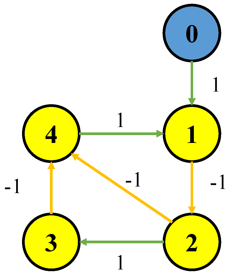
2.1. Graph Theory

This paper considers a network of agents consisting of one leader and N followers. The leader is denoted as agent 0, and the followers are denoted as agents 1 to N. The interactions among the N agents are represented by a directed graph $\mathcal{G}=(\mathcal{V},\mathcal{E},\mathcal{A})$, where $\mathcal{V}=v_1,\cdots ,v_N$ is the set of nodes, $\mathcal{E}=(v_i,v_j)\subset \mathcal{V}\times \mathcal{V}$ is the set of edges, and $\mathcal{A}={\left[a_{ij}\right]}_{N\times N}$ is the adjacency matrix. If agent i can access the information of agent j, then $a_{ij}\ne 0$; otherwise, $a_{ij}=0$. $a_{ij}>0$ and $a_{ij}<0$, respectively, represent the cooperative and competitive relationships between agents i and j. If $a_{ij}\ne a_{ji}$, the graph is directed; otherwise, it is undirected. The Laplacian matrix is defined as $L=D-\mathcal{A}$, where $D={\mathbf{diag}}_i^N\left[{\zeta }_i\right],$ with ${\zeta }_i={\displaystyle \sum _{j=1}^N}\left|a_{ij}\right|$. The in-degree matrix D is a diagonal matrix, and for a directed graph, the diagonal elements of the in-degree matrix ${\zeta }_i$ are the sums of the corresponding row in the adjacency matrix. An additional leader agent is introduced, with the node set ${\mathcal{V}}_0=v_0$, and the overall node set is $\overline{\mathcal{V}}=\mathcal{V}\cup {\mathcal{V}}_0$.

For a structurally balanced signed graph $\overline{\mathcal{V}}$, the node set can be divided into two mutually exclusive subsets ${\overline{\mathcal{V}}}_1$ and ${\overline{\mathcal{V}}}_2$. The signature matrix $\Delta$ is defined as $\Delta ={\mathbf{diag}}_i^n\left[d_i\right]$, where, if ${\mathcal{V}}_0\in {\overline{\mathcal{V}}}_q$, then $\forall v_i\in {\overline{\mathcal{V}}}_q,d_i=1$, indicating a cooperative relationship between the followers and the leader; otherwise, $d_i=-1$, indicating an antagonistic relationship. $B={\mathbf{diag}}_i^N\left[b_i\right]$, where if the i-th agent is aware of the leader’s information, then $b_i>0$; otherwise, $b_i=0$. The extended Laplacian matrix is $\overline{L}=L+B$, which describes the communication topology between the leader and the followers.

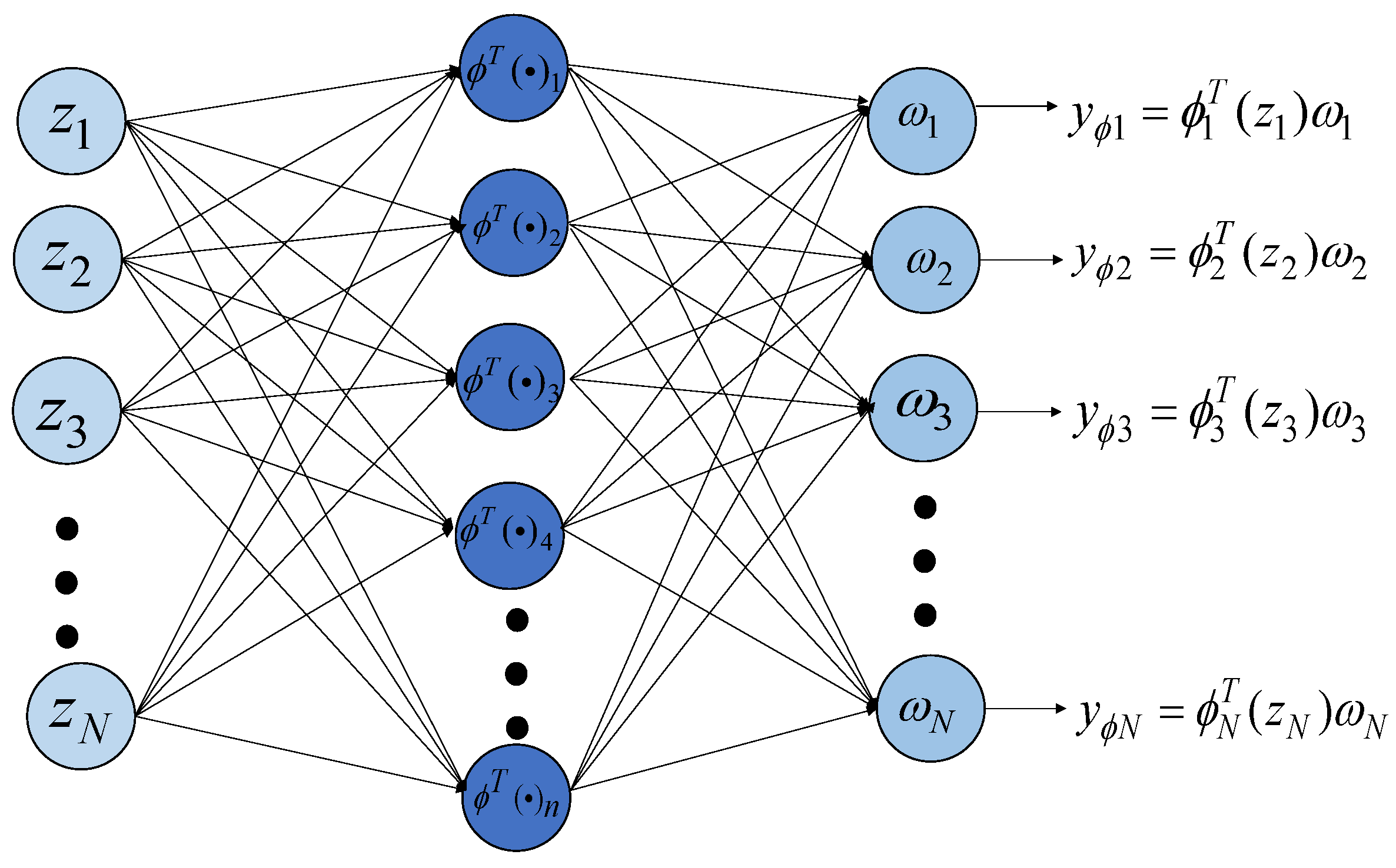
2.2. RBF Neural Network

Radial basis function (RBF) neural networks adjust centers and widths to approximate unknown functions. Figure 1 depicts a typical structure of neural networks, clearly illustrating the weighted process from input to output.

Neural networks often utilize Gaussian functions as their basis functions, which take the form ${\varphi }_{ij}\left(z\right)=exp(-{\displaystyle \frac{{∥z-c_{ij}∥}^2}{{\delta }_{ij}^2}})$, where z represents the input vector, while $\sigma$ and c are the width and center parameters of the Gaussian function, respectively. This approach enables the approximation of continuous functions with arbitrary precision over compact sets. The neural network’s output is represented by $y={\varphi }^T\left(z\right)\omega$. Crucially, neural networks possess innate function approximation capabilities that are unaffected by the inherent properties of the system being modeled. By employing a sufficient number of Gaussian functions, this neural network architecture can approximate continuous functions to an arbitrary degree of accuracy within compact domains. When designing controllers for systems with model uncertainties or disturbances, leveraging neural networks for estimation can enhance the overall robustness of the control system.

The following

Table 1. Parameters and their meanings.

Symbol	Meaning
q	leader’s state
y	leader’s output
$Q\left(w\right)$	the leader’s state matrix
w	an unknown parameter vector
E	the leader’s output matrix
$q_i,{\dot{q}}_i,{\ddot{q}}_i$	the generalized coordinate, velocity, and acceleration
$M_i\left(q_i\right)$	the inertia matrix
$C_i(q_i,{\dot{q}}_i)$	the Coriolis and centrifugal terms
$G_i\left(q_i\right)$	the vector of gravitational force
$u_i$	the control input
$f_i(q_i,{\dot{q}}_i,{\ddot{q}}_i)$	the unknown external disturbance
$p_i{u}_i$	the actuator fault
${\widehat{q}}_i$	the estimations of q
${\widehat{y}}_i$	the estimations of y
${\widehat{w}}_i$	the estimations of w
${\widehat{E}}_i$	the estimations of E
${\zeta }_i$	the column vector of output matrix observation errors
${\widehat{p}}_i$	the estimation of $p_i^{\ast }=1/p_i$
$e_{1i},e_{2i}$	the tracking error vectors
$\chi ={[\varphi ,\theta ,\psi ]}^T$	the attitude vector of the quadrotor rigid body
$\tilde{q}$	the estimation errors of q
$\tilde{w}$	the estimation errors of w

lists some important parameters and their meanings in this article.

2.3. Problem Description

Considering a networked agent system composed of one leader and N followers. The following linear system models the leader.

$$\begin{array}{cc}\hfill & \dot{q}=Q\left(w\right)q,\hfill \\ \hfill & y=Eq,\hfill \end{array}$$

(1)

where $q\in {\Re }^m$ and $y\in {\Re }^n$ denote the leader’s state and output. $Q\left(w\right)$ represents the state matrix, where $w\in {\Re }^l$ is an unknown parameter vector. Moreover, $E\in {\Re }^{n\times m}$ denotes the output matrix, which is unknown to any follower.

The following Euler–Lagrange equation is utilized to describe the dynamics of the ith follower.

$$\begin{array}{ccc}\hfill M_i\left(q_i\right){\ddot{q}}_i+C_i(q_i,{\dot{q}}_i){\dot{q}}_i+G_i\left(q_i\right)& =p_i{u}_i+f_i(q_i,{\dot{q}}_i,{\ddot{q}}_i),\hfill & \hfill i=1,2,\dots N,\end{array}$$

(2)

where $q_i,{\dot{q}}_i,{\ddot{q}}_i\in {\Re }^n$ are the generalized coordinate, velocity, and acceleration, respectively. $M_i\left(q_i\right)\in {\Re }^{n\times n}$ is the inertia matrix, $C_i(q_i,{\dot{q}}_i)\in {\Re }^{n\times n}$ represents the Coriolis and centrifugal terms, $G_i\left(q_i\right)\in {\Re }^n$ is the vector of gravitational force, $u_i\in {\Re }^n$ is the control input, and $f_i(q_i,{\dot{q}}_i,{\ddot{q}}_i)\in {\Re }^n$ represents the unknown external disturbance. $p_i$ is an unknown constant. And $p_i{u}_i$ represents the actuator fault. In this paper, it is assumed that $M_i\left(q_i\right)$, $C_i(q_i,{\dot{q}}_i)$, and $G_i\left(q_i\right)$ are unknown to any follower.

The dynamics (2) exhibit the following two properties [30].

Property 1. 

$M_i\left(q_i\right)$ is symmetric and positive definite.

Property 2. 

${\dot{M}}_i\left(q_i\right)-2C_i(q_i,{\dot{q}}_i)$ is skew-symmetric, i.e., for all $x\in {\Re }^n$, it yields $x^T[{\dot{M}}_i\left(q_i\right)-2C_i(q_i,{\dot{q}}_i)]x=0$.

To realize the bipartite consensus tracking, it is necessary to give the following assumptions.

Assumption 1. 

A connected, structure-balanced, and directed graph can be used to model the communication topology of the networked MASs. In addition, it also ensures that at least one follower will be informed about the information given by the leader.

Assumption 2. 

The eigenvalues of $Q\left(w\right)$ are all simple with zero real components.

Under Assumption 2, it is assumed that

$$Q\left(w\right)={\mathbf{diag}}_i^l\left[w_i\right]\otimes v,$$

(3)

where $v=\left[\begin{array}{cc}0& 1\\ -1& 0\end{array}\right]$. It can be obtained that $Q\left(w\right)$ is a skew-symmetric matrix.

Remark 1. 

Assumption 2 is rather standard in the literature on consensus tracking of networked systems [31,32]. Under Assumption 2, the leader agent (1) can generate a set of signals commonly seen in the industry, known as “multitone sinusoidal signals” with varying frequencies, amplitudes, and initial phases, which align more closely with real-world scenarios [33,34]. The application scenario of the control scheme in this paper is the signal tracking of Euler–Lagrange systems in complex sea conditions. Hence, the control objective of this paper is to make the follower ’s state $q_i$ and the leader ’s output y tend to be consistent.

Lemma 1 

([35]). For any $\alpha \in {\Re }^l$ and $\delta ,\varpi \in {\Re }^{2l},$ we define

$$\phi \left(\varpi \right)=\left[\begin{array}{cccc}-{\varpi }_2& {\varpi }_1& \cdots & 0\\ ⋮& \ddots & \ddots & ⋮\\ 0& \cdots & -{\varpi }_{2l}& {\varpi }_{2l-1}\end{array}\right],$$

and then the following equation holds:

$$\begin{array}{c}\phi \left(\varpi \right)\delta =-\phi \left(\delta \right)\varpi ,\hfill \\ Q\left(\alpha \right)\varpi =-{\phi }^T\left(\varpi \right)\alpha ,\hfill \end{array}$$

where $Q\left(\alpha \right)={\mathit{diag}}_i^l\left[{\alpha }_i\right]\otimes v,v=\left[\begin{array}{cc}0& 1\\ -1& 0\end{array}\right],$ and $\alpha ={\mathit{col}}_i^l\left[{\alpha }_i\right],\varpi ={\mathit{col}}_i^{2l}\left[{\alpha }_i\right],\delta ={\mathit{col}}_i^{2l}\left[{\delta }_i\right].$

Lemma 2 

([22]). Under Assumption 1, there exists a positive diagonal matrix $W\in {\Re }^{N\times N}$ such that $W\overline{L}$ can be diagonalized and possesses eigenvalues that are both real and positive. Moreover, there exists a symmetric positive definite matrix $O\in {\Re }^{N\times N}$ such that

$$J=OW\overline{L},T=JW\overline{L}+{\overline{L}}^{T}WJ$$

(4)

are symmetric positive definite.

Remark 2. 

The analysis of networked systems on undirected graphs hinges upon the symmetry exhibited by specific matrices, such as the Laplacian matrix, which reflects the symmetric topology characterizing undirected graphs. However, the asymmetry of the Laplacian matrix presents a primary challenge when analyzing networked systems on directed graphs. Lemma 2 presents a method for constructing two symmetric matrices, J and O, derived from the asymmetric matrix $\overline{L}$. By employing these two symmetric matrices in the formulation of Lyapunov equations, it becomes feasible to extend the control scheme from undirected graphs to encompass directed graphs.

Definition 1. 

Consider the leader–follower systems (1) and (2). If the equation

$$\underset{t\to \infty }{lim}(q_i\left(t\right)-d_{i}y\left(t\right))=0,i=1,\dots N,$$

holds, then the leader–follower MASs (1) and (2) will achieve the bipartite consensus tracking.

3. Neural-Network-Based Control Scheme Design and Analysis

The control scheme comprises a distributed observer and a neural-network-based robust controller. The design and analysis details of the aforementioned two parts are as follows.

3.1. Distributed Observer Design and Stability Analysis

In this part, we will design a distributed observer to estimate the leader’s dynamic information.

Firstly, we define the observation error vectors as

$$\begin{array}{cc}\hfill e_{q_i}& =\sum _{j=1}^N\left|a_{ij}\right|({\widehat{q}}_j-\mathrm{sgn}\left(a_{ij}\right){\widehat{q}}_i)+b_i(q-{\widehat{q}}_i),\hfill \\ \hfill e_{yi}& =\sum _{j=1}^N\left|a_{ij}\right|({\widehat{y}}_j-\mathrm{sgn}\left(a_{ij}\right){\widehat{y}}_i)+b_i(y-{\widehat{y}}_i),\hfill \end{array}$$

(5)

where ${\widehat{q}}_i$ and ${\widehat{y}}_i$ represent the estimations of q and y.

Then, the distributed observer is constructed in the following way:

$$\begin{array}{c}{\dot{\widehat{q}}}_i=H\left({\widehat{w}}_i\right){\widehat{q}}_i+{\rho }_1{\eta }_i{e}_{q_i},\hfill \\ {\dot{\widehat{w}}}_i={\rho }_2{\eta }_i\phi \left(e_{q_i}\right){\widehat{q}}_i,\hfill \\ {\dot{\widehat{E}}}_i={\eta }_i{e}_{yi}{\widehat{q}}_i^T,\hfill \end{array}$$

(6)

where ${\widehat{w}}_i$ and ${\widehat{E}}_i$ represent the estimations of w and E. Parameters ${\rho }_1$, ${\rho }_2$ and ${\eta }_i$ will be specified later. And ${\widehat{y}}_i={\widehat{E}}_i{\widehat{q}}_i.$

Remark 3. 

As shown in (6), the distributed observer proposed in this paper estimates the leader’s state q, the unknown parameter w, and the output matrix E, respectively, where w and E are globally unknown. Compared with the works of [28,36,37,38,39,40,41,42,43,44], which assume that some of the leader’s dynamic information, such as the state matrix or the output matrix, is accessible to uninformed agents, observer (6) is more consistent with the characteristics of distributed networked systems and can be applied to tracking scenarios with complex leader dynamics, such as rotating machinery tasks and operations in complex sea conditions.

We define the estimation errors as ${\tilde{q}}_i={\widehat{q}}_i-d_{i}q,\tilde{w}={\widehat{w}}_i-w$, and ${\tilde{E}}_i={\widehat{E}}_i-E$. The objective of designing the observer (6) is to make the following equations hold:

$$\begin{array}{c}\underset{t\to \infty }{lim}{\tilde{q}}_i\left(t\right)=0,\hfill \\ \underset{t\to \infty }{lim}{\tilde{w}}_i\left(t\right)=0,\hfill \\ \underset{t\to \infty }{lim}{\tilde{E}}_i\left(t\right)=0.\hfill \end{array}$$

(7)

Let $W={\mathbf{diag}}_i^N\left[{\eta }_i\right]$, $e_q={\mathbf{col}}_i^N\left[e_{q_i}\right]$, $\overline{q}={\mathbf{1}}_N\otimes q$, $\overline{w}={\mathbf{1}}_N\otimes w,$$\widehat{w}={\mathbf{col}}_i^N\left[{\widehat{w}}_i\right]$, and $\widehat{q}={\mathbf{col}}_i^N\left[{\widehat{q}}_i\right].$ Then, we can obtain the result that

$$\begin{array}{cc}\hfill \dot{\widehat{q}}& =\overline{Q}\left(\widehat{w}\right)\widehat{q}+{\rho }_1(W\otimes I_m)e_q,\hfill \\ \hfill \dot{\widehat{w}}& ={\rho }_2\overline{\phi }\left(e_q\right)(W\otimes I_m)\widehat{q},\hfill \\ \hfill e_q& =-(\overline{L}\otimes I_m)(\widehat{q}-\overline{q}),\hfill \end{array}$$

(8)

where

$$\begin{array}{c}\overline{\phi }\left(e_q\right)={\mathbf{diag}}_i^N\left[\phi \left(e_{qi}\right)\right],\hfill \\ \overline{Q}\left(\widehat{w}\right)={\mathbf{diag}}_i^N\left[Q\left({\widehat{w}}_i\right)\right].\hfill \end{array}$$

Then, it yields

$$\begin{array}{cc}\hfill \dot{\widehat{q}}& =\overline{Q}\left(\widehat{w}\right)\widehat{q}-{\rho }_1(W\overline{L}\otimes I_m)(\widehat{q}-\overline{q}),\hfill \\ \hfill \dot{\widehat{w}}& ={\rho }_2\overline{\phi }\left(e_q\right)(W\otimes I_m)\widehat{q}.\hfill \end{array}$$

(9)

Remark 4. 

To solve the asymmetric issue of $\overline{L}$, we introduce the positive definite diagonal matrix W in (6), which is constructed in Lemma 2. We utilize two symmetric positive definite matrices J and O to design the Lyapunov Equation (16), thus extending the control scheme from undirected topologies to generally directed topologies.

We define $\tilde{q}={\mathbf{col}}_i^N\left[{\tilde{q}}_i\right]$ and $\tilde{w}={\mathbf{col}}_i^N\left[{\tilde{w}}_i\right]$. It can be obtained that

$$\begin{array}{c}\dot{\tilde{q}}=(I_N\otimes Q\left(w\right)-{\rho }_{1}W\overline{L}\otimes I_m)\tilde{q}+\overline{H}\left(\tilde{w}\right)\widehat{q},\hfill \\ \dot{\tilde{w}}={\rho }_2\overline{\phi }\left(e_q\right)(W\otimes I_m)\widehat{q}.\hfill \end{array}$$

(10)

According to Lemma 1, we have

$$\begin{array}{c}\dot{\tilde{q}}=(I_N\otimes Q\left(w\right)-{\rho }_{1}W\overline{L}\otimes I_m)\tilde{q}-{\overline{\phi }}^T\left(\widehat{q}\right)\tilde{w},\hfill \\ \dot{\tilde{w}}={\rho }_2\overline{\phi }\left(\widehat{q}\right)(W\overline{L}\otimes I_m)\tilde{q},\hfill \end{array}$$

(11)

where $\overline{\phi }\left(\widehat{q}\right)={\mathbf{diag}}_i^N\left[\phi \left({\widehat{q}}_i\right)\right].$ By derivation of $\tilde{E}$, we can obtain the result that

$${\dot{\tilde{E}}}_i={\eta }_i\sum _{j=0}^N{a}_{ij}({\tilde{E}}_j-{\tilde{E}}_i)q{q}^T+{\chi }_i\left(t\right),$$

(12)

where ${\chi }_i\left(t\right)={\eta }_i{\displaystyle \sum _{j=0}^N}{a}_{ij}\left(({\tilde{E}}_j-{\tilde{E}}_i)q{\tilde{q}}_i^T\right)+{\eta }_{i}E{e}_{q_i}{\widehat{q}}_i^T+{\eta }_i{\displaystyle \sum _{j=0}^N}{a}_{ij}({\tilde{E}}_j{\tilde{q}}_j{\widehat{q}}_i^T-{\tilde{E}}_i{\tilde{q}}_i{\widehat{q}}_i^T).$

Define the column vector of output matrix observation errors ${\varsigma }_i=\mathbf{Col}\left[{\tilde{E}}_i\right],{\varsigma }_0=\mathbf{Col}\left[E\right]$ and ${\xi }_i=\mathbf{Col}\left[{\chi }_i\left(t\right)\right]$; then Equation (11) turns to

$${\dot{\varsigma }}_i=(q{q}^T\otimes I_n){\eta }_i\sum _{j=0}^N{a}_{ij}({\varsigma }_j-{\varsigma }_i)+{\xi }_i,$$

(13)

where ${\xi }_i\left(t\right)={\eta }_i{\displaystyle \sum _{j=0}^N}{a}_{ij}\left[({\tilde{q}}_i{q}^T\otimes I_n)({\varsigma }_j-{\varsigma }_i)\right)+({\widehat{q}}_i{\tilde{q}}_j^T\otimes I_n){\varsigma }_j-({\widehat{q}}_i{\tilde{q}}_i^T\otimes I_m){\varsigma }_j]+{\eta }_i({\widehat{q}}_i{e}_{qi}^T\otimes I_n){\varsigma }_0.$ Define $\varsigma ={\mathbf{col}}_i^N\left[{\varsigma }_i\right]$ and $\xi {=\mathbf{col}}_i^N\left[{\xi }_i\right]$, which yields

$$\begin{array}{c}\hfill \dot{\varsigma }=-(I_N\otimes (q{q}^T\otimes I_n))(W\overline{L}\otimes I_{nm})\varsigma +\xi =-(W\overline{L}\otimes (q{q}^T\otimes I_n))\varsigma +\xi .\end{array}$$

(14)

Based on the above derivation using coordinate transformation, the objective of Section 3.2 is to investigate the stability of the systems (11) and (14) to demonstrate the convergence of the observer (6).

In this part, we will investigate the stability of the systems (11) and (14).

Theorem 1. 

Consider systems (1) and (6). Define two compact sets ${{\rm Y}}_0\subset {\Re }^m$ and ${{\rm Y}}_1\subset {\Re }^l$ with $0\in {{\rm Y}}_0,0\in {{\rm Y}}_1$. Under Assumptions 1 and 2, for any ${\widehat{w}}_i\left(0\right)\in {{\rm Y}}_0,w\in {{\rm Y}}_0,{\widehat{q}}_i\left(0\right)\in {{\rm Y}}_1,q\left(0\right)\in {{\rm Y}}_1$, ${\rho }_2>0$, then it yields that

$$\begin{array}{c}\underset{t\to \infty }{lim}\tilde{q}\left(t\right)=0,\hfill \\ \underset{t\to \infty }{lim}\tilde{w}\left(t\right)=0.\hfill \end{array}$$

(15)

Proof. 

The Lyapunov function is employed as

$$V={\tilde{q}}^T(J\otimes I_m)\tilde{q}+{\rho }_2^{-1}{\tilde{w}}^T(O\otimes I_l)\tilde{w},$$

(16)

where $J\in {\Re }^{N\times N}$ and $O\in {\Re }^{N\times N}$ are mentioned in Lemma 2. $\tilde{q}$ values represent the estimation errors of q. $\tilde{w}$ values represent the estimation errors of w. $I_m$ and $I_l$ represent identity matrixes. ${\rho }_2$ represents a constant. Then, it yields

$$\begin{array}{cc}\hfill \dot{V}=& 2{\tilde{q}}^T(J\otimes Q\left(w\right))\tilde{q}-{\rho }_1{\tilde{q}}^T((JW\overline{L}+{\overline{L}}^{T}WJ)\otimes I_m)\tilde{q}-2{\tilde{q}}^T(J\otimes I_m){\overline{\phi }}^T\left(\tilde{q}\right)\tilde{w}-\hfill \\ & 2{\tilde{q}}^T(J\otimes I_m){\overline{\phi }}^T\left(\overline{q}\right)\tilde{w}+2{\rho }_2^{-1}{\tilde{w}}^T(O\otimes I_l)\dot{\tilde{w}}.\hfill \end{array}$$

(17)

Given the skew-symmetric property of $Q\left(w\right)$ and the symmetry of J, it follows that $J\otimes Q\left(w\right)$ is also skew-symmetric. Subsequently, we have

$$\begin{array}{c}\hfill \dot{V}=-{\rho }_1{\tilde{q}}^T(T\otimes I_m)\tilde{q}-2{\tilde{q}}^T(J\otimes I_m)){\overline{\phi }}^T\left(\tilde{q}\right)\tilde{w}-2{\tilde{q}}^T(J\otimes {\phi }^T\left(q\right))\tilde{w}+2{\rho }_2^{-1}{\tilde{w}}^T(O\otimes I_l)\dot{\tilde{w}}.\end{array}$$

(18)

Substituting (11) into (18), we can obtain the result that

$$\begin{array}{cc}\hfill \dot{V}=& -{\rho }_1{\tilde{q}}^T(T\otimes I_m)\tilde{q}-2{\tilde{q}}^T(J\otimes I_m)){\overline{\phi }}^T\left(\tilde{q}\right)\tilde{w}-2{\tilde{q}}^T(J\otimes {\phi }^T\left(q\right))\tilde{w}\hfill \\ & +2{\tilde{w}}^T(O\otimes I_l)\overline{\phi }\left(\widehat{q}\right)(W\overline{L}\otimes I_m)\tilde{q}\hfill \\ \hfill =& -{\rho }_1{\tilde{q}}^T(T\otimes I_m)\tilde{q}-2{\tilde{q}}^T(J\otimes I_m)){\overline{\phi }}^T\left(\tilde{q}\right)\tilde{w}+2{\tilde{w}}^T(O\otimes I_l)\overline{\phi }\left(\tilde{q}\right)(W\overline{L}\otimes I_m)\tilde{q}\hfill \\ & +2{\tilde{w}}^T(OW\overline{L}\otimes \phi \left(q\right))\tilde{q}-2{\tilde{q}}^T(J\otimes {\phi }^T\left(q\right))\tilde{w}.\hfill \end{array}$$

(19)

Based on Lemma 2, it yields

$$\begin{array}{c}\hfill {\tilde{w}}^T(OW\overline{L}\otimes \phi \left(q\right))\tilde{q}={\tilde{q}}^T(J\otimes \phi \left(q\right))\tilde{w}.\end{array}$$

(20)

From Equation (19) and (20), we can obtain the result that

$$\begin{array}{cc}\hfill \dot{V}=& -{\rho }_1{\tilde{q}}^T(T\otimes I_m)\tilde{q}-2{\tilde{q}}^T(J\otimes I_m)){\overline{\phi }}^T\left(\tilde{q}\right)\tilde{w}+2{\tilde{w}}^T(O\otimes I_l)\overline{\phi }\left(\tilde{q}\right)(W\overline{L}\otimes I_m)\tilde{q}\hfill \\ \hfill \le & -{\rho }_1{\tilde{q}}^T(T\otimes I_m)\tilde{q}+2∥\tilde{w}∥∥\overline{\phi }\left(\tilde{q}\right)∥∥(J\otimes I_m)∥∥\tilde{q}∥\hfill \\ & +2∥\tilde{w}∥∥(O\otimes I_l)∥∥\overline{\phi }\left(\tilde{q}\right)∥∥(W\overline{L}\otimes I_m)∥∥\tilde{q}∥.\hfill \end{array}$$

(21)

According to Property 9.4.11 in [45], we can obtain the result that $∥\overline{\phi }\left(\tilde{q}\right)∥\le ∥\mathbf{Col}[\overline{\phi }\left(\tilde{q}\right)]∥=∥\tilde{q}∥$. Then it yields

$$\begin{array}{cc}\hfill \dot{V}& \le -{\rho }_1{\tilde{q}}^T(T\otimes I_m)\tilde{q}+2∥\tilde{w}∥∥J∥{∥\tilde{q}∥}^2+2∥\tilde{w}∥∥O∥∥W\overline{L}∥{∥\tilde{q}∥}^2.\hfill \end{array}$$

(22)

Define $r^{\ast }=2∥J∥+2∥O∥∥W\overline{L}∥$, and the smallest eigenvalue of the matrix T is denoted as ${\lambda }_T$. Then, according to Lemma 2, it follows that

$$\begin{array}{c}\hfill \dot{V}\le -({\rho }_1{\lambda }_T-r^{\ast }∥\tilde{w}\left(t\right)∥){∥\tilde{q}∥}^2.\end{array}$$

(23)

According to Lemma 7 in [22], $\tilde{w}\left(t\right)$ is uniformly bounded. Define ${\tilde{w}}^{\ast }=sup\left\{∥\tilde{w}\left(t\right)∥\right\}$ and ${\rho }_1^{\ast }={\displaystyle \frac{{\tilde{w}}^{\ast }{r}^{\ast }+1}{{\lambda }_T}}$. Then, we can obtain the result that for ${\rho }_1\ge {\rho }_1^{\ast }$,

$$\begin{array}{c}\hfill \dot{V}\le -{∥\tilde{q}∥}^2.\end{array}$$

(24)

Therefore, we can obtain the result that $\dot{V}$ is negative semidefinite and $\underset{t\to \infty }{lim}\tilde{q}\left(t\right)=0$.

Next, we will demonstrate the convergence of $\tilde{w}\left(t\right)$. According to (10), it yields

$$\ddot{\tilde{q}}=(I_N\otimes Q\left(w\right)-{\rho }_{1}W\overline{L}\otimes I_m)\dot{\tilde{q}}-{\overline{\phi }}^T\left(\widehat{q}\right)\dot{\tilde{w}}-{\overline{\phi }}^T\left(\dot{\widehat{q}}\right)\tilde{w}.$$

Since $\tilde{q}$, $\tilde{w}$, and $\widehat{q}$ are uniformly bounded (see Lemma 6 in [22]), according to (9) and (11), we have $\dot{\tilde{q}}$, $\dot{\tilde{w}}$, and $\dot{\widehat{q}}$, which are also uniformly bounded. Therefore, $\ddot{\tilde{q}}$ is uniformly bounded. By applying Barbalat’s lemma, we have $\underset{t\to \infty }{lim}\dot{\tilde{q}}\left(t\right)=0$. From $\underset{t\to \infty }{lim}\tilde{q}\left(t\right)=0$ and (10), we can obtain the result that

$$\underset{t\to \infty }{lim}{\overline{\phi }}^T\left(\widehat{q}\right)\tilde{w}\left(t\right)=0,\underset{t\to \infty }{lim}{\tilde{w}}^T\left(t\right)\overline{\phi }\left(\widehat{q}\right){\overline{\phi }}^T\left(\widehat{q}\right)\tilde{w}\left(t\right)=0.$$

From Lemma 7 in [22], it yields that for ${\rho }_1\ge {\rho }_1^{\ast }$, the following inequality holds

$${\varpi }_1{I}_m\ge {\displaystyle \frac{1}{T}}{\int }_t^{t+T}\overline{\phi }\left(\widehat{q}\right){\overline{\phi }}^T\left(\widehat{q}\right)d\widehat{q}\ge {\varpi }_0{I}_m,\forall t\ge T_0,$$

where ${\varpi }_1,{\varpi }_0,T_0,T$ are positive constants. Then, according to Lemma 1 in [46], we can obtain the result that $\underset{t\to \infty }{lim}\tilde{w}\left(t\right)=0$. □

Theorem 2. 

Consider systems (1) and (6). Define two compact sets ${{\rm Y}}_0\subset {\Re }^m$ and ${{\rm Y}}_1\subset {\Re }^l$ with $0\in {{\rm Y}}_0,0\in {{\rm Y}}_1$. Under Assumptions 1 and 2, for any ${\widehat{w}}_i\left(0\right)\in {{\rm Y}}_0,w\in {{\rm Y}}_0,{\widehat{q}}_i\left(0\right)\in {{\rm Y}}_1,q\left(0\right)\in {{\rm Y}}_1$, ${\rho }_2>0$, it yields the result that $\underset{t\to \infty }{lim}{\tilde{E}}_i\left(t\right)=0.$

Proof. 

Firstly, we consider system (14) with $\xi =0$ as

$$\begin{array}{c}\hfill \dot{\varsigma }=-(W\overline{L}\otimes (q\left(t\right)q^T\left(t\right)\otimes I_n))\varsigma .\end{array}$$

(25)

According to Lemma 2, since $W\overline{L}$ can be diagonalized and possesses eigenvalues that are real and positive, there exists a matrix $M_H$ such that $M_{H}W\overline{L}{M}_H^{-1}={\mathbf{diag}}_i^N\left[{\lambda }_{ui}\right]=K_H,$ where ${\lambda }_{ui}>0$ are eigenvalues of $W\overline{L}$. Define $k_h=(M_H\otimes I_{nm})\varsigma$, so Equation (25) can be transformed as

$$\begin{array}{c}\hfill {\dot{k}}_h=-(K_H\otimes (q\left(t\right)q^T\left(t\right)\otimes I_n))k_h.\end{array}$$

(26)

Define $-(W\overline{L}\otimes (q\left(t\right)q^T\left(t\right)\otimes I_N))=\overline{B}$, so Equation (25) can be simplified to

$$\begin{array}{c}\hfill \dot{\varsigma }=\overline{B}\varsigma .\end{array}$$

(27)

According to Lemma 1 in [32], $q\left(t\right)$ satisfies the following inequality:

$$\begin{array}{c}\hfill b_1{I}_m\ge {\int }_t^{t+T_0}q\left(\tau \right)q^T\left(\tau \right)d\tau \ge b_2{I}_m,\end{array}$$

(28)

where $b_1,b_2$ and $T_0$ are positive constants. Furthermore, we can obtain the result that

$$\begin{array}{c}\hfill b_1{K}_H\otimes I_{nm}\ge {\int }_t^{t+T_0}{K}_H\otimes (q\left(\tau \right)q^T\left(\tau \right)\otimes I_n)d\tau \ge b_2{K}_H\otimes I_{nm}.\end{array}$$

(29)

From Theorem 1 in [47], it can be deduced that system (26) is asymptotically stable. Equivalently, system (25) is also asymptotically stable. Therefore, for a positive definite matrix $F_1\left(t\right)$ satisfying $∥F_1\left(t\right)∥\ge l_3$, where $l_3$ is a positive constant. There exists a positive definite matrix $k_h\left(t\right)$ that satisfies $l_1\le ∥k_h\left(t\right)∥\le l_2$, where $l_1$ and $l_2$ are positive constants. The subsequent equation holds:

$$\begin{array}{c}\hfill {\dot{k}}_h\left(t\right)=-k_h\left(t\right)\overline{B}\left(t\right)-{\overline{B}}^T\left(t\right)k_h\left(t\right)-F_1\left(t\right).\end{array}$$

(30)

Next, we analyze system (14) with $\xi \ne 0$. Construct the following Lyapunov function:

$$\begin{array}{c}\hfill V_a={\varsigma }^T{k}_h\left(t\right)\varsigma .\end{array}$$

(31)

Then, we can obtain the result that

$$\begin{array}{cc}\hfill {\dot{V}}_a& ={\varsigma }^T({\dot{Z}}_1\left(t\right)+k_h\left(t\right)\overline{B}\left(t\right)+{\overline{B}}^T\left(t\right)k_h\left(t\right))\varsigma +2{\varsigma }^T{k}_h\left(t\right)\xi =-{\varsigma }^T{F}_1\left(t\right)\varsigma +2{\varsigma }^T{k}_h\left(t\right)\xi \hfill \\ & \le -l_3{∥\xi ∥}^2+2∥k_h\left(t\right)∥∥\varsigma ∥∥\xi ∥.\hfill \end{array}$$

(32)

From Lemma 6 in [22], we have ${\widehat{q}}_i$, which is uniformly bounded. Furthermore, for $q\left(0\right)\in {\Re }^m$ in system (1), we have $q\left(t\right)=e^{Q\left(w\right)t}q\left(0\right)$. According to Assumption 2, it yields $∥q\left(t\right)∥=∥q\left(0\right)∥$. There exists a sufficiently large constant $q_m$ such that $∥\widehat{q}\left(t\right)∥\le q_m$ and $∥q∥\le q_m$. According to Equation (13), we have

$$\begin{array}{cc}\hfill ∥{\xi }_i∥\le & {\eta }_i(\sum _{j=0}^N{a}_{ij}∥({\tilde{q}}_i{q}^T\otimes I_n)({\varsigma }_j-{\varsigma }_i)∥+∥({\widehat{q}}_i{e}_{qi}^T\otimes I_n){\varsigma }_0∥\hfill \\ & +\sum _{j=0}^N{a}_{ij}∥({\widehat{q}}_i{\tilde{q}}_j^T\otimes I_n){\varsigma }_j-({\widehat{q}}_i{\tilde{q}}_i^T\otimes I_m){\varsigma }_i∥)\hfill \\ \hfill \le & {\eta }_i(\sum _{j=0}^N{a}_{ij}∥({\tilde{q}}_i{q}^T\otimes I_n)∥∥({\varsigma }_j-{\varsigma }_i)∥+∥({\widehat{q}}_i{e}_{qi}^T\otimes I_n)∥∥{\varsigma }_0∥+\sum _{j=0}^N{a}_{ij}(∥{\widehat{q}}_i{\tilde{q}}_j^T\otimes I_n∥∥{\varsigma }_j∥\hfill \\ & +∥{\widehat{q}}_i{\tilde{q}}_i^T\otimes I_m∥∥{\varsigma }_i∥\left)\right)\hfill \\ \hfill \le & {\eta }_i(2\sum _{j=0}^N{a}_{ij}∥{\tilde{q}}_i{q}^T∥∥\varsigma ∥+\sum _{j=0}^N{a}_{ij}∥{\widehat{q}}_i{e}_{qi}^T∥∥\varsigma ∥+\sum _{j=0}^N{a}_{ij}∥{\widehat{q}}_i{\tilde{q}}_i^T∥∥\varsigma ∥+∥{\widehat{q}}_i{e}_{qi}^T∥∥E∥)\hfill \\ \hfill \le & {\eta }_i(q_m∥\varsigma ∥\sum _{j=0}^N{a}_{ij}(3∥{\tilde{q}}_i∥+∥{\tilde{q}}_j∥)+q_m∥e_{qi}∥∥E∥)le{\eta }_i(4q_m∥\varsigma ∥∥\tilde{q}∥\sum _{j=0}^N{a}_{ij}+q_m∥e_{qi}∥∥E∥).\hfill \end{array}$$

(33)

Since $∥\xi \left(t\right)∥\le {\displaystyle \sum _{i=1}^N}∥{\xi }_i\left(t\right)∥$, it yields

$$\begin{array}{c}\hfill ∥\xi \left(t\right)∥\le \eta (∥\varsigma \left(t\right)∥{\chi }_0\left(t\right)+{\chi }_1\left(t\right)),\end{array}$$

(34)

where $\eta ={\mathbf{col}}_i^N\left[{\eta }_i\right]$, ${\chi }_0\left(t\right)=4q^m∥\tilde{q}\left(t\right)∥{\displaystyle \sum _{i=0}^N}{\displaystyle \sum _{j=0}^N}{a}_{ij}$, and ${\chi }_1\left(t\right)=N{q}^m∥E∥∥e_q\left(t\right)∥.$ Substituting into Equation (32), it follows that

$$\begin{array}{cc}\hfill {\dot{V}}_a& \le -l_3{∥\varsigma ∥}^2+2\alpha l_2{∥\varsigma ∥}^2{\chi }_0\left(t\right)+2\alpha l_2∥\varsigma ∥{\chi }_1\left(t\right)\hfill \\ & \le -l_3{∥\varsigma ∥}^2+2\alpha l_2{∥\varsigma ∥}^2{\chi }_0\left(t\right)+{\displaystyle \frac{\alpha l_3}{4}}{∥\varsigma ∥}^2+{\displaystyle \frac{4\alpha l_2^2}{c_3}}{\chi }_1^2\left(t\right)\hfill \\ \hfill & =-{\displaystyle \frac{(4-\alpha )l_3}{4}}{∥\varsigma ∥}^2+2l_2{\chi }_0\left(t\right){∥\varsigma ∥}^2+{\displaystyle \frac{{\chi }_1^2\left(t\right)}{w_h}}\hfill \\ & \le -({\displaystyle \frac{(4-\alpha )l_3}{4l_2}}-{\displaystyle \frac{2l_2{\chi }_0\left(t\right)}{l_1}})V_a+{\displaystyle \frac{{\chi }_1^2\left(t\right)}{w_h}},\hfill \end{array}$$

(35)

where $w_h={\displaystyle \frac{l_3}{4l_2^2}}$, and from Theorem 1, we have $\underset{t\to \infty }{lim}{\chi }_1\left(t\right)={\chi }_0\left(t\right)=0$. Since $l_3$ and $l_2$ are positive constants, as long as we ensure that ${\eta }_i$ is no larger than 4, it can be obtained that ${\dot{V}}_a$ is negative definite. Therefore, we have $\underset{t\to \infty }{lim}\varsigma \left(t\right)=0$.

The proof is completed. □

Remark 5. 

According to Theorem 1 and 2, we can obtain the result that the following equations hold: $\underset{t\to \infty }{lim}{\tilde{q}}_i=\underset{t\to \infty }{lim}{\tilde{w}}_i=\underset{t\to \infty }{lim}{\tilde{E}}_i=\underset{t\to \infty }{lim}{\tilde{y}}_i=\widehat{y_i}-d_{i}y$ and $\underset{t\to \infty }{lim}{e}_{qi}=\underset{t\to \infty }{lim}{e}_{yi}=0$.

3.2. Robust Tracking Controller Design and Stability Analysis

We will propose a neural-network-based robust controller to let the tracking error converge to zero in this part. In the meantime, adaptive update laws are devised to ensure the boundedness of the estimation errors of lumped uncertainties composed of unknown matrices and external disturbances in the follower model.

Firstly, we define the tracking error vectors as

$$\begin{array}{cc}\hfill e_{1i}& =q_i-{\widehat{y}}_i,\hfill \\ \hfill e_{2i}& ={\dot{q}}_i-{\beta }_i,\hfill \end{array}$$

(36)

where ${\beta }_i={\widehat{E}}_{i}Q\left({\widehat{w}}_i\right){\widehat{q}}_i-K_{1i}{e}_{1i}$ and $K_{1i}$ is a positive definite matrix. Subsequently, we need to estimate the following lumped uncertainty composed of unknown matrices and external disturbances in the follower model.

$$\begin{array}{c}\hfill {\delta }_i=-G_i-C_i{\beta }_i-M_i{\dot{\beta }}_i+f_i.\end{array}$$

(37)

For the sake of simplicity, we assume that the lumped uncertainty ${\delta }_i$ can be formulated over a designated compact set ${\Omega }_f\subset {\Re }^r$ and using a neural network as

$$\begin{array}{c}\hfill {\delta }_i(q_i,{\dot{q}}_i)={\varphi }_i^T(q_i,{\dot{q}}_i){\omega }_i+{\varpi }_{fi},\end{array}$$

(38)

where ${\varphi }_i^T(q_i,{\dot{q}}_i)\in {\Re }^{r\times b}$ is the basis function, and ${\omega }_i\in {\Re }^b$ is an unknown parameter vector. ${\varpi }_{fi}$ is the neural network estimation error, which is bounded by a vector ${\chi }_{fi}$, that is, $∥{\varpi }_{fi}∥\le {\chi }_{fi}$. The estimation of ${\omega }_i$ is represented as ${\widehat{\omega }}_i\left(t\right)$. The estimated value of ${\delta }_i$ is represented as ${\widehat{\delta }}_i$. Then, ${\widehat{\delta }}_i$ can be represented as follows:

$$\begin{array}{cc}\hfill {\widehat{\delta }}_i(q_i,{\dot{q}}_i)& ={\varphi }_i^T(q_i,{\dot{q}}_i){\widehat{\omega }}_i\left(t\right).\hfill \end{array}$$

(39)

The estimation errors are defined as ${\tilde{\omega }}_i={\omega }_i-{\widehat{\omega }}_i$ and ${\tilde{\delta }}_i={\delta }_i-{\widehat{\delta }}_i$. To achieve the approximation of the follower to the dynamic of the leader, the compact set of states can be determined based on the sensor’s initial rough estimate of the distance between the leader and the follower. This generates a compact set with a wide range initially. Then, the compact set range can be continuously adjusted to optimize the neural network model.

Remark 6. 

As shown in Equation (37), ${\delta }_i$ is a lumped uncertainty composed of unknown matrices and external disturbances in the follower model. Neural networks are employed to estimate the lumped uncertainty ${\delta }_i$ online and design a feedforward term ${\varphi }_i^T{\widehat{\omega }}_i$ in the controller (40) to compensate it, thus improving the robustness of the system.

The neural-network-based robust controller is designed as follows:

$$\begin{array}{cc}\hfill u_i& =-{\widehat{p}}_i(K_{2i}{e}_{2i}+e_{1i}+{\varphi }_i^T{\widehat{\omega }}_i+{\tau }_i\mathrm{sgn}\left(e_{2i}\right)),\hfill \end{array}$$

(40)

where ${\widehat{p}}_i$ is the estimation of $p_i^{\ast }={\displaystyle \frac{1}{p_i}}$. $K_{2i}$ is a positive definite matrix, and ${\tau }_i$ is a positive constant satisfying ${\tau }_i\ge {\chi }_{fi}$.

The adaptive update laws are designed as follows:

$$\begin{array}{cc}\hfill {\dot{\widehat{\omega }}}_i& =m_f{\varphi }_i^T{e}_{2i},\hfill \\ \hfill {\dot{\widehat{p}}}_i& =-e_{2i}{\theta }_i,\hfill \end{array}$$

(41)

where $m_f$ is a positive constant and ${\theta }_i=K_{2i}{e}_{2i}+e_{1i}+{\varphi }_i^T{\widehat{\omega }}_i+{\tau }_i\mathrm{sgn}\left(e_{2i}\right)$. Then, we define ${\tilde{p}}_i=p_i^{\ast }-{\widehat{p}}_i$ and ${\overline{p}}_i=p_i{\tilde{p}}_i{\theta }_i$.

Remark 7. 

The design of the neural-network-based robust controller comprises three components. The state feedback term $-K_{2i}{e}_{2i}-e_{1i}$ serves to realize the fundamental functions of the controller. The neural network estimation feedforward term $-{\varphi }_i^T{\widehat{\omega }}_i$ is employed to enhance the stability of the system. The term $-\tau i\mathrm{sgn}\left(e_{2i}\right)$ is utilized to mitigate the impact of neural network estimation errors on the system.

To summarize, the control strategy of the closed-loop tracking control system is illustrated in the diagram shown in Figure 2. The control scheme proposed in this paper consists of a distributed observer and a neural-network-based robust controller. For the leader model (1) with uncertain parameters w and uncertain output matrix E, a distributed observer (6) is proposed to estimate the global information of the leader (1). On this basis, the estimations of the leader information ${\widehat{w}}_i$, ${\widehat{q}}_i$, ${\widehat{E}}_i$, and ${\widehat{y}}_i$ are substituted into the neural-network-based robust controller (40). Then, we design adaptive update laws (41) to ensure the effectiveness of the neural network estimation of the lumped uncertainty. We can see that the estimations ${\widehat{w}}_i$, ${\widehat{q}}_i$ and ${\widehat{E}}_i$ obtained through the distributed observer (6) play a role in the adaptive laws.

Theorem 3. 

Consider the leader–follower systems (1) and (2). Suppose Assumptions 1 and 2 hold. If the neural-network-based robust controller and adaptive update laws are designed as (40) and (41), then the leader–follower systems (1) and (2) will achieve consensus tracking.

Proof. 

By the derivation of $e_{1i}$ and $e_{2i}$, we can obtain the result that

$$\begin{array}{cc}\hfill {\dot{e}}_{1i}& =e_{2i}+{\beta }_i-{\dot{\widehat{y}}}_i,\hfill \\ \hfill {\dot{e}}_{2i}& ={\ddot{q}}_i-{\dot{\beta }}_i.\hfill \end{array}$$

(42)

Consider the Lyapunov function as

$$\begin{array}{c}\hfill V_{bi}={\displaystyle \frac{1}{2}}{e}_{1i}^T{e}_{1i}.\end{array}$$

(43)

By the derivation of (43), and according to (42), it yields

$$\begin{array}{c}\hfill {\dot{V}}_{bi}=-e_{1i}^T{K}_{1i}{e}_{1i}+e_{1i}^T{e}_{2i}+e_{1i}^T({\widehat{E}}_{i}Q\left({\widehat{w}}_i\right){\widehat{q}}_i-{\dot{\widehat{y}}}_i).\end{array}$$

(44)

Substituting (42) into (2), it can be obtained that

$$\begin{array}{c}\hfill M_i{\dot{e}}_{2i}+C_i{e}_{2i}=u_i+{\delta }_i.\end{array}$$

(45)

Then, we consider the second Lyapunov function as

$$\begin{array}{c}\hfill V_{ci}=V_{bi}+{\displaystyle \frac{1}{2}}{e}_{2i}^T{M}_i{e}_{2i}.\end{array}$$

(46)

Then, we have

$$\begin{array}{cc}\hfill {\dot{V}}_{ci}& =-e_{1i}^T{K}_{1i}{e}_{1i}+e_{1i}^T{e}_{2i}+e_{1i}^T({\widehat{E}}_{i}Q\left({\widehat{w}}_i\right){\widehat{q}}_i-{\dot{\widehat{y}}}_i)+{\displaystyle \frac{1}{2}}{e}_{2i}^T{\dot{M}}_i\left(q_i\right)e_{2i}+e_{2i}^T{M}_i\left(q_i\right){\dot{e}}_{2i}.\hfill \end{array}$$

(47)

Substituting (45) into (47), and according to Property 2, it follows that

$$\begin{array}{cc}\hfill {\dot{V}}_{ci}& =-e_{1i}^T{K}_{1i}{e}_{1i}+e_{1i}^T{e}_{2i}+e_{1i}^T({\widehat{E}}_{i}Q\left({\widehat{w}}_i\right){\widehat{q}}_i-{\dot{\widehat{y}}}_i)+e_{2i}^T(u_i+{\delta }_i).\hfill \end{array}$$

(48)

Then, we consider the third Lyapunov function as

$$\begin{array}{c}\hfill V_{di}=V_{ci}+{\displaystyle \frac{{\tilde{\omega }}_i^T{\tilde{\omega }}_i}{2m_f}}+\sum _{i=1}^N{\displaystyle \frac{p_i{\left({\tilde{p}}_i\right)}^2}{2}}.\end{array}$$

(49)

Then, we have

$$\begin{array}{c}\hfill {\dot{V}}_{di}={\dot{V}}_{ci}-{\displaystyle \frac{{\tilde{\omega }}_i^T{\dot{\widehat{\omega }}}_i}{m_f}}-\sum _{i=1}^N{p}_i{\tilde{p}}_i{\dot{\tilde{p}}}_i\end{array}$$

(50)

Substituting (38), (40), (48) into (50), we can obtain the result that

$$\begin{array}{cc}\hfill {\dot{V}}_{di}=& -e_{1i}^T{K}_{1i}{e}_{1i}+e_{1i}^T{e}_{2i}+e_{1i}^T({\widehat{E}}_{i}Q\left({\widehat{w}}_i\right){\widehat{q}}_i-{\dot{\widehat{y}}}_i)+e_{2i}^T(-K_{2i}{e}_{2i}-e_{1i}-{\varphi }_i^T{\widehat{\omega }}_i-{\tau }_i\mathrm{sgn}\left(e_{2i}\right)\hfill \\ & +{\varphi }_i^T{\omega }_i+{\varpi }_{fi}+{\overline{p}}_i)-\sum _{i=1}^N{p}_i{\tilde{p}}_i{\dot{\tilde{p}}}_i-{\displaystyle \frac{{\tilde{\omega }}_i^T{\dot{\widehat{\omega }}}_i}{m_f}}\hfill \\ \hfill =& -e_{1i}^T{K}_{1i}{e}_{1i}+e_{1i}^T{e}_{2i}+e_{1i}^T({\widehat{E}}_{i}Q\left({\widehat{w}}_i\right){\widehat{q}}_i-{\dot{\widehat{y}}}_i)-e_{2i}^T{K}_{2i}{e}_{2i}-e_{2i}^T{e}_{1i}-e_{2i}^T{\varphi }_i^T{\widehat{\omega }}_i-e_{2i}^T{\tau }_i\mathrm{sgn}\left(e_{2i}\right)\hfill \\ & +e_{2i}^T{\varphi }_i^T{\omega }_i+e_{2i}^T{\varpi }_{fi}-{\displaystyle \frac{{\tilde{\omega }}_i^T{\dot{\widehat{\omega }}}_i}{m_f}}+e_{2i}^T{\overline{p}}_i-\sum _{i=1}^N{p}_i{\tilde{p}}_i{\dot{\tilde{p}}}_i\hfill \\ \hfill =& -e_{1i}^T{K}_{1i}{e}_{1i}-e_{2i}^T{K}_{2i}{e}_{2i}+e_{1i}^T({\widehat{E}}_{i}Q\left({\widehat{w}}_i\right){\widehat{q}}_i-{\dot{\widehat{y}}}_i)-e_{2i}^T{\tau }_i\mathrm{sgn}\left(e_{2i}\right)+e_{2i}^T{\varphi }_i^T{\tilde{\omega }}_i\hfill \\ & +e_{2i}^T{\varpi }_{fi}-{\displaystyle \frac{{\tilde{\omega }}_i^T{\dot{\widehat{\omega }}}_i}{m_f}}+e_{2i}^T{\overline{P}}_i-\sum _{i=1}^N{p}_i{\tilde{p}}_i{\dot{\tilde{p}}}_i.\hfill \end{array}$$

(51)

Substituting (41) into (51), it yields

$$\begin{array}{cc}\hfill {\dot{V}}_{di}& =-e_{1i}^T{K}_{1i}{e}_{1i}-e_{2i}^T{K}_{2i}{e}_{2i}+e_{1i}^T({\widehat{E}}_{i}Q\left({\widehat{w}}_i\right){\widehat{q}}_i-{\dot{\widehat{y}}}_i)-e_{2i}^T{\tau }_i\mathrm{sgn}\left(e_{2i}\right)+e_{2i}^T{\varpi }_{fi}\hfill \\ \hfill & \le -e_{1i}^T{K}_{1i}{e}_{1i}-e_{2i}^T{K}_{2i}{e}_{2i}+e_{1i}^T({\widehat{E}}_{i}Q\left({\widehat{w}}_i\right){\widehat{q}}_i-{\dot{\widehat{y}}}_i)-{\tau }_i∥e_{2i}∥+∥e_{2i}∥∥{\varpi }_{fi}∥\hfill \\ \hfill & \le -e_{1i}^T{K}_{1i}{e}_{1i}-e_{2i}^T{K}_{2i}{e}_{2i}+e_{1i}^T({\widehat{E}}_{i}Q\left({\widehat{w}}_i\right){\widehat{q}}_i-{\dot{\widehat{y}}}_i)-{\tau }_i∥e_{2i}∥+∥e_{2i}∥{\chi }_{fi}\hfill \\ \hfill & \le -e_{1i}^T{K}_{1i}{e}_{1i}-e_{2i}^T{K}_{2i}{e}_{2i}+e_{1i}^T({\widehat{E}}_{i}Q\left({\widehat{w}}_i\right){\widehat{q}}_i-{\dot{\widehat{y}}}_i).\hfill \end{array}$$

(52)

From (6), we have

$$\begin{array}{cc}\hfill {\dot{V}}_{di}& \le -e_{1i}^T{K}_{1i}{e}_{1i}-e_{2i}^T{K}_{2i}{e}_{2i}+e_{1i}^T({\widehat{E}}_{i}Q\left({\widehat{w}}_i\right){\widehat{q}}_i-{\dot{\widehat{E}}}_i{\widehat{q}}_i-{\widehat{E}}_i{\dot{\widehat{q}}}_i)\hfill \\ & =-e_{1i}^T{K}_{1i}{e}_{1i}-e_{2i}^T{K}_{2i}{e}_{2i}+e_{1i}^T({\widehat{E}}_{i}Q\left({\widehat{w}}_i\right){\widehat{q}}_i-{\eta }_i{e}_{yi}{\widehat{q}}_i^T{\widehat{q}}_i-{\widehat{E}}_{i}Q\left({\widehat{w}}_i\right){\widehat{q}}_i-{\widehat{E}}_i{\rho }_1{\eta }_i{e}_{q_i})\hfill \\ & =-e_{1i}^T{K}_{1i}{e}_{1i}-e_{2i}^T{K}_{2i}{e}_{2i}+e_{1i}^T(-e_{yi}{\eta }_i{\widehat{q}}_i^T{\widehat{q}}_i-{\widehat{E}}_i{\rho }_1{\eta }_i{e}_{q_i}),\hfill \end{array}$$

(53)

where $e_{q_i}$ and $e_{y_i}$ are the observation errors defined in (5). According to Remark 5, we have $\underset{t\to \infty }{lim}{e}_{qi}=\underset{t\to \infty }{lim}{e}_{yi}=\underset{t\to \infty }{lim}{\tilde{y}}_i=0$. Since $K_{1i}$ and $K_{2i}$ are positive definite, it yields $\underset{t\to \infty }{lim}{\dot{V}}_{di}\le -e_{1i}^T{K}_{1i}{e}_{1i}-e_{2i}^T{K}_{2i}{e}_{2i}$; that is, ${\dot{V}}_{di}$ is negative definite when t tends to infinity. Therefore, it yields $\underset{t\to \infty }{lim}{e}_{1i}\left(t\right)=\underset{t\to \infty }{lim}{e}_{2i}\left(t\right)=0$. Then, we have $\underset{t\to \infty }{lim}{e}_{1i}=\underset{t\to \infty }{lim}{q}_i-{\widehat{y}}_i=\underset{t\to \infty }{lim}{q}_i-d_{i}y=0$. Based on Definition 1, the leader–follower systems described by Equations (1) and (2) can reach bipartite consensus tracking. The proof is finished. □

4. Simulation Results

Numerical simulations are carried out in this part. Two different simulation models are employed to verify the designed consensus tracking control protocol through simulation; one is a two-link robot manipulator, and the other is a mathematical model of a quadrotor drone. The results are shown below.

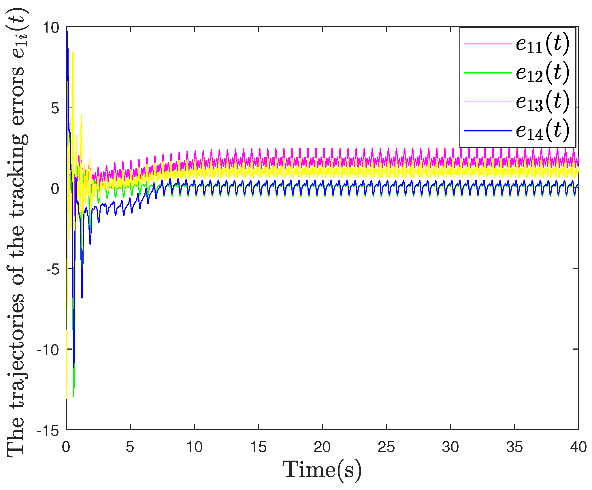
4.1. Example 1: Two-Link Robot Manipulator

A two-link robot manipulator benchmark model is used for simulation in this subsection, as shown in Figure 3.

Based on the Euler–Lagrange mechanism, the manipulator model is obtained given by

$$\begin{array}{ccc}\hfill M_i\left(q_i\right){\ddot{q}}_i+C_i(q_i,{\dot{q}}_i){\dot{q}}_i+G_i\left(q_i\right)& =p_i{u}_i+f_i(q_i,{\dot{q}}_i,{\ddot{q}}_i),\hfill & \hfill i=1,2,\dots 4,\end{array}$$

where

$$\begin{array}{cc}\hfill q_i& =\mathbf{col}[q_{i1},q_{i2}],M_i\left(q_i\right)=\left[\begin{array}{cc}{d}_{i1}+d_{i2}+2d_{i3}\cos \left(q_{i2}\right)& d_{i2}+2d_{i3}\cos \left(q_{i2}\right)\\ d_{i2}+2d_{i3}\cos \left(q_{i2}\right)& d_{i2}\end{array}\right],\hfill \\ \hfill C_i(q_i,{\dot{q}}_i)& =\left[\begin{array}{cc}-d_{i3}\sin \left(q_{i2}\right){\dot{q}}_{i2}& -d_{i3}\sin \left(q_{i2}\right)({\dot{q}}_{i1}+{\dot{q}}_{i2})\\ d_{i3}\sin \left(q_{i2}\right){\dot{q}}_{i1}& 0\end{array}\right],\hfill \\ \hfill G_i\left(q_i\right)& =\left[\begin{array}{c}{d}_{i4}g\cos \left(q_{i1}\right)+d_{i4}g\cos (q_{i1}+q_{i2})\\ d_{i5}g\cos (q_{i1}+q_{i2})\end{array}\right],\hfill \\ \hfill d_{i1}& =J_{i1}+m_{i2}{l}_{i1}^2,d_{i2}=0.25m_{i2}{l}_{i2}^2+J_{i2},d_{i3}=0.5m_{i2}{l}_{i1}{l}_{i2},d_{i4}=(0.5m_{i1}+m_{i2})l_{i1},\hfill \\ \hfill d_{i5}& =0.5m_{i2}{l}_{i2},f_i(q_i,{\dot{q}}_i,{\ddot{q}}_i)=5\%·[M_i\left(q_i\right){\ddot{q}}_i+C_i(q_i,{\dot{q}}_i){\dot{q}}_i+G_i\left(q_i\right)],\hfill \end{array}$$

g = 9.8 m/s² is the gravitational acceleration. $m_{i1}$, $m_{i2}$ are masses of links. $l_{i1}$ denotes lengths of links. $l_{i2}$ represents the distance from the center of the mass to the joints. $J_{i1}$ and $J_{i2}$ denote moments of inertia of links. $d_{i1}$~$d_{i5}$ represent different constant values in the inertia matrix, Coriolis and centrifugal force matrix, and gravity force vector. $q_i=\mathbf{col}[q_{i1},q_{i2}]$ represent the different joint angle positions of the two mechanical arms of the robotic manipulator, where i represents the $i_{th}$ agent. We consider a group of two-link manipulators consisting of four followers. The communication topology among manipulators is shown in Figure 4. The first follower can obtain the information of the leader. Simulation parameters are given in

Table 2. Parameters of two-link manipulators.

Parameter	Manipulator 1	Manipulator 2	Manipulator 3	Manipulator 4
$l_{i1}$ (m)	0.98	1	0.96	1
$l_{i2}$ (m)	1	0.95	1	1.02
$m_{i1}$ (kg)	1.02	0.96	1.01	1.04
$m_{i2}$ (kg)	1.12	1.15	1.07	1.09
$J_{i1}$ (kg · m2)	0.23	0.21	0.19	0.21
$J_{i2}$ (kg · m2)	0.41	0.4	0.42	0.41

. The initial values are selected as follows:

$$\begin{array}{cc}\hfill q_{11}\left(0\right)& =5\pi ,q_{12}\left(0\right)=-5\pi ,q_{21}\left(0\right)=10\pi ,q_{22}\left(0\right)=-5\pi ,q_{31}\left(0\right)=15\pi ,q_{32}\left(0\right)=5\pi ,\hfill \\ \hfill q_{41}\left(0\right)& =20\pi ,q_{42}\left(0\right)=5\pi ,p_1=0.98,p_2=0.95,p_3=0.9,p_4=0.92,{\dot{q}}_{i1}\left(0\right)={\dot{q}}_{i2}\left(0\right)=0,\hfill \\ \hfill q\left(0\right)& =\mathbf{col}(2,0.6,2,0.8,2,1).\hfill \end{array}$$

The following linear system is used to represent the dynamics of the leader, which can denote a signal generator in complex sea conditions under Assumption 2.

$$\begin{array}{c}\dot{q}=Q\left(w\right)q,\hfill \\ y=Eq.\hfill \end{array}$$

The leader’s system matrices are set as:

$$w=\mathbf{col}[2,5,8],E=\left[\begin{array}{cccccc}0.1& 0& 0.2& 0& 0.3& 0\\ 0& 0.3& 0& 0.2& 0& 0.1\end{array}\right].$$

The activation functions of each follower are described as

$${\varphi }_{1i}\left(z\right)={\varphi }_{2i}\left(z\right)={[{\varphi }_{i1}\left(z\right),\dots ,{\varphi }_{i6}\left(z\right)]}^T.$$

In this paper, we choose Gaussian functions as activation functions. The details are as follows: ${\varphi }_{ij}\left(z\right)=exp(-{\displaystyle \frac{{∥z-c_{ij}∥}^2}{{\delta }_{ij}^2}}),j=1,\dots ,6,$ where $z={\left[q_i,{\dot{q}}_i,{\beta }_i\right]}^T\in {\Re }^6$. We assume that all the followers have the same activation functions. $c_{ij}$ represents the center of the receptive field, which is evenly distributed in ${\left[-5,5\right]}^4\times {\left[-0.5,0.5\right]}^2$. ${\delta }_{ij}=2$ is the width of the Gaussian function. The initial weights ${\widehat{\omega }}_{1i}$ and ${\widehat{\omega }}_{2i}$ are chosen as ${\widehat{\omega }}_{1i}\left(0\right)={\widehat{\omega }}_{2i}\left(0\right)={\mathbf{0}}_{6\times 2}$. The control parameters are selected as $K_{1i}=K_{2i}=40I_2,{\tau }_i=10,{\rho }_1=80,$ and ${\rho }_2=60$. We select $W=\mathbf{diag}({\alpha }_1,\dots {\alpha }_N)=\mathbf{diag}(1,2,3,4)$. In order to show the numerical simulations intuitively, we define ${\overline{q}}_{0i}=∥{\tilde{q}}_i∥,{\overline{w}}_i=∥{\tilde{w}}_i∥,$ and ${\overline{E}}_i=∥{\tilde{E}}_i∥$.

Table 3. The comparison results.

The Tracking Errors	Overall Performance $\overline{\mathit{e}}$ and $\mathit{\delta }$	Overall Performance in [22] $\overline{\mathit{e}}$ and $\mathit{\delta }$	Steady-State Performance $\overline{\mathit{e}}$ and $\mathit{\delta }$	Steady-State Performance in [22] $\overline{\mathit{e}}$ and $\mathit{\delta }$
$e_{11}$	−0.039, 0.280	0.979, 1.475	−0.006, 0.008	1.623, 0.325
$e_{12}$	0.065, 0.652	0.571, 1.760	−0.003, 0.009	1.360, 0.324
$e_{13}$	0.072, 0.972	0.473, 1.708	−0.006, 0.014	1.062, 0.322
$e_{14}$	−0.011, 1.192	0.091, 1.595	0.006, 0.014	1.322, 0.366

lists the comparison results between this article and [22].

In Table 3, $\overline{e}$ represents the average value of the tracking errors, and $\delta$ represents the standard deviation of the tracking errors. By comparison, it can be observed that the method adopted in this paper results in smaller tracking errors and also smaller fluctuation ranges, thereby enhancing the robustness of the system.

The systems described by Equations (1) and (2) can achieve bipartite consensus tracking, as illustrated in Figure 5. Furthermore, Figure 6 demonstrates the convergence of the tracking errors of the networked agent system to zero. Figure 6 and Figure 7 indicate that the distributed observer (6) can effectively estimate the leader’s dynamic information, including the state q, the unknown parameter w, and the output matrix E. The control inputs shown in Figure 8 indicate that by using neural networks, the estimation errors of the lumped uncertainties ${\delta }_i$ are bounded.

To highlight this paper’s contribution, we compare it with article [22], a leading work in the consensus tracking of an uncertain leader under directed graphs. We introduce the same external disturbance $f_i$ to the follower model in article [22] and compare the results by observing the figures of tracking errors (Figure 6 and Figure 9).

Remark 8. 

Figure 6 and Figure 9 show that the neural-network-based robust controller proposed in this paper effectively suppresses external disturbances and enhances the robustness of the system. Compared with the control strategy in article [22], the proposed scheme offers notable research significance in real-world applications.

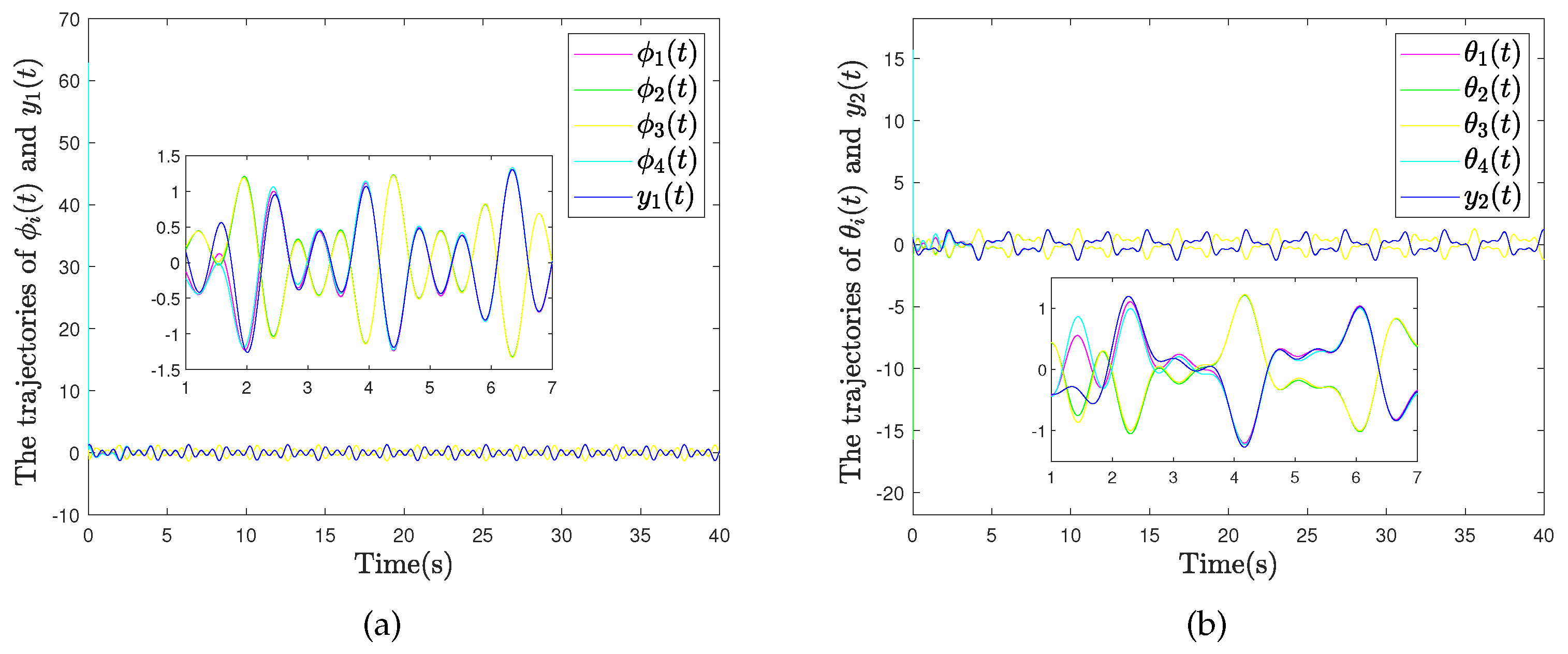
4.2. Example 2: Quadrotor Drone

In this subsection, a mathematical model of a quadrotor drone is utilized for simulation as follows:

$$M_i\left({\chi }_i\right){\ddot{\chi }}_i+C_i({\chi }_i,{\dot{\chi }}_i){\dot{\chi }}_i=u_{\chi i}+f_{\chi i}$$

(54)

where ${\chi }_i={[{\varphi }_i,{\theta }_i,{\psi }_i]}^T$ denotes the attitude vector of the quadrotor rigid body expressed in the inertial frame. The matrix $C_i({\chi }_i,\dot{{\chi }_i})$ is the Coriolis term containing the gyroscopic and centrifugal terms, and $M_i\left({\chi }_i\right)$ is the inertia matrix. $u_{\chi i}$ is the total control torque for the rotational motion, $f_{\chi i}$ denotes the disturbance torque. The explicit expression of $M_i\left({\chi }_i\right)$ and $C_i({\chi }_i,\dot{{\chi }_i})$ can be seen in [48].

The following linear system is used to represent the dynamics of the leader, which can denote a signal generator in complex sea conditions under Assumption 2.

$$\begin{array}{c}\dot{q}=Q\left(w\right)q,\hfill \\ y=Eq.\hfill \end{array}$$

The leader’s system matrices are set as

$$w=\mathbf{col}[2,5,8],E=\left[\begin{array}{cccccc}0.1& 0& 0.2& 0& 0.3& 0\\ 0& 0.3& 0& 0.2& 0& 0.1\\ 0.1& 0.3& 0.2& 0.2& 0.1& 0.2\end{array}\right].$$

The rest of the control parameters are the same as in Example 1. We define the tracking error vectors as ${\tilde{\varphi }}_i={\varphi }_i-d_i{y}_1,{\tilde{\theta }}_i={\theta }_i-d_i{y}_2$, and ${\tilde{\psi }}_i={\psi }_i-d_i{y}_3$.

In order to verify that the proposed control scheme’s adaptability enhances its applicability to a wider array of consensus tracking control tasks, we conduct an additional set of experiments by altering the output matrix of the leader system. The leader’s output matrix is set as

$$E=\left[\begin{array}{cccccc}0.5& 0.1& 0.1& 0.1& 0.1& 0.2\\ 0.1& 0.5& 0.1& 0.1& 0.3& 0.1\\ 0.1& 0.1& 0.5& 0.1& 0.1& 0.3\end{array}\right]$$

As shown in Figure 10, Figure 11, Figure 12 and Figure 13, the systems described by (1) and (54) can achieve bipartite consensus tracking. Figure 11 and Figure 13, Figure 14 and Figure 15 indicate that the tracking errors of attitudes of quadrotor drones converge to zero.

5. Conclusions

This paper has investigated the bipartite consensus tracking problem for networked ELSs with an uncertain leader agent across directed topologies. The ELSs under consideration are afflicted by unknown dynamic matrices, external disturbances, and actuator faults. A novel control strategy, integrating a distributed observer with a neural-network-based robust controller, has been devised. Neural networks are employed to approximate the lumped uncertainties, which include unknown matrices and external disturbances within the follower model. The distributed observer is tailored to estimate the leader’s dynamic information. Adaptive update laws have been formulated for the unknown parameters within the neural networks and the actuator fault factors, ensuring the boundedness of the estimation errors. A neural-network-based robust controller is proposed to ensure that tracking errors asymptotically converge to zero. Numerical simulations have been conducted to substantiate the efficacy of the proposed control strategy. In future work, we will delve into the bipartite consensus tracking control scheme with event-triggered communications, which is anticipated to further enhance the efficiency and practicality of the system.

References

1. Dong, J.; Yassine, A.; Armitage, A.; Hossain, M.S. Multi-Agent Reinforcement Learning for Intelligent V2G Integration in Future Transportation Systems. IEEE Trans. Intell. Transp. Syst. 2023, 1, 15974–15983. [Google Scholar] [CrossRef]
2. Xu, D.; Chen, G. The research on intelligent cooperative combat of UAV cluster with multi-agent reinforcement learning. Aerosp. Syst. 2022, 5, 107–121. [Google Scholar] [CrossRef]
3. Wang, H.; Tao, J.; Peng, T.; Brintrup, A.; Kosasih, E.E.; Lu, Y.; Tang, R.; Hu, L. Dynamic inventory replenishment strategy for aerospace manufacturing supply chain: Combining reinforcement learning and multi-agent simulation. Int. J. Prod. Res. 2022, 60, 4117–4136. [Google Scholar] [CrossRef]
4. Peng, X.J.; He, Y.; Chen, W.H.; Liu, Q. Bipartite consensus tracking control for periodically-varying-delayed multi-agent systems with uncertain switching topologies. Commun. Nonlinear Sci. Numer. Simul. 2023, 121, 107226. [Google Scholar] [CrossRef]
5. Wang, H.; Han, Q.L. Distribution of Roots of Quasi-Polynomials of Neutral Type and Its Application-Part II: Consensus Protocol Design of Multi-Agent Systems Using Delayed State Information. IEEE Trans. Autom. Control 2023, 69, 4058–4065. [Google Scholar] [CrossRef]
6. Zhao, M.; Peng, C.; Tian, E. Finite-time and fixed-time bipartite consensus tracking of multi-agent systems with weighted antagonistic interactions. IEEE Trans. Circuits Syst. I Regul. Pap. 2020, 68, 426–433. [Google Scholar] [CrossRef]
7. Wang, B.; Chen, W.; Zhang, B. Semi-global robust tracking consensus for multi-agent uncertain systems with input saturation via metamorphic low-gain feedback. Automatica 2019, 103, 363–373. [Google Scholar] [CrossRef]
8. Wang, W.; Wen, C.; Huang, J. Distributed adaptive asymptotically consensus tracking control of nonlinear multi-agent systems with unknown parameters and uncertain disturbances. Automatica 2017, 77, 133–142. [Google Scholar] [CrossRef]
9. Wang, X.; Niu, B.; Zhang, J.; Wang, H.; Jiang, Y.; Wang, D. Adaptive Event-Triggered Consensus Tracking Control Schemes for Uncertain Constrained Nonlinear Multi-Agent Systems. IEEE Trans. Autom. Sci. Eng. 2023. [Google Scholar] [CrossRef]
10. Ren, Z.; Lin, B.; Shi, M.; Li, Z.; Qin, K. UDE-based Consensus Tracking Control of Multi-Agent Systems with Actuator Faults and External Disturbances. In Proceedings of the 2023 6th International Conference on Electronics Technology (ICET), Chengdu, China, 12–15 May 2023; pp. 1282–1288. [Google Scholar]
11. Qin, J.; Zhang, G.; Zheng, W.X.; Kang, Y. neural-network-based adaptive consensus control for a class of nonaffine nonlinear multiagent systems with actuator faults. IEEE Trans. Neural Netw. Learn. Syst. 2019, 30, 3633–3644. [Google Scholar]
12. Bo, Z.; Wei, W.; Hao, Y. Distributed consensus tracking control of linear multi-agent systems with actuator faults. In Proceedings of the 2014 IEEE Conference on Control Applications (CCA), Juan Les Antibes, France, 8–10 October 2014; pp. 2141–2146. [Google Scholar]
13. Lu, X.; Wang, Y.; Yu, X.; Lai, J. Finite-time control for robust tracking consensus in MASs with an uncertain leader. IEEE Trans. Cybern. 2016, 47, 1210–1223. [Google Scholar] [CrossRef] [PubMed]
14. Lui, D.G.; Petrillo, A.; Santini, S. Bipartite tracking consensus for high-order heterogeneous uncertain nonlinear multi-agent systems with unknown leader dynamics via adaptive fully-distributed PID control. IEEE Trans. Netw. Sci. Eng. 2022, 10, 1131–1142. [Google Scholar] [CrossRef]
15. Tahoun, A.; Arafa, M. Adaptive leader–follower control for nonlinear uncertain multi-agent systems with an uncertain leader and unknown tracking paths. ISA Trans. 2022, 131, 61–72. [Google Scholar] [CrossRef] [PubMed]
16. Zhang, G.; Cheng, D. Adaptive fault-tolerant guaranteed performance control for Euler–Lagrange systems with its application to a 2-link robotic manipulator. IEEE Access 2020, 8, 184160–184171. [Google Scholar] [CrossRef]
17. Liang, Z.; Wen, H.; Yao, B.; Mao, Z.; Lian, L. Adaptive actuator fault and the abnormal value reconstruction for marine vehicles with a class of Euler–Lagrange system. Ocean Eng. 2024, 297, 117095. [Google Scholar] [CrossRef]
18. Wei, C.; Luo, J.; Dai, H.; Yuan, J. Adaptive model-free constrained control of postcapture flexible spacecraft: A Euler–Lagrange approach. J. Vib. Control 2018, 24, 4885–4903. [Google Scholar] [CrossRef]
19. Lu, M.; Liu, L. Leader–following consensus of multiple uncertain Euler–Lagrange systems with unknown dynamic leader. IEEE Trans. Autom. Control 2019, 64, 4167–4173. [Google Scholar] [CrossRef]
20. Dong, Y.; Chen, Z. Fixed-time synchronization of networked uncertain Euler–Lagrange systems. Automatica 2022, 146, 110571. [Google Scholar] [CrossRef]
21. Mei, J.; Ren, W.; Ma, G. Distributed coordinated tracking with a dynamic leader for multiple Euler–Lagrange systems. IEEE Trans. Autom. Control 2011, 56, 1415–1421. [Google Scholar] [CrossRef]
22. Wang, S.; Zhang, H.; Chen, Z. Adaptive cooperative tracking and parameter estimation of an uncertain leader over general directed graphs. IEEE Trans. Autom. Control 2022, 68, 3888–3901. [Google Scholar] [CrossRef]
23. Cheng, B.; Li, Z. Coordinated tracking of Euler–Lagrange systems over directed graphs via distributed continuous controllers. In Proceedings of the 2016 35th Chinese Control Conference (CCC), Chengdu, China, 27–29 July 2016; pp. 8144–8149. [Google Scholar]
24. Miyasato, Y. Adaptive H-inf consensus control of Euler–Lagrange systems on directed network graph. In Proceedings of the 2016 IEEE Symposium Series on Computational Intelligence (SSCI), Athens, Greece, 6–9 December 2016; pp. 1–6. [Google Scholar]
25. Deng, Q.; Peng, Y.; Han, T.; Qu, D. Event-triggered bipartite consensus in networked Euler–Lagrange systems with external disturbance. IEEE Trans. Circuits Syst. II Express Briefs 2021, 68, 2870–2874. [Google Scholar] [CrossRef]
26. Li, B.; Han, T.; Xiao, B.; Zhan, X.S.; Yan, H. Leader-following bipartite consensus of multiple uncertain Euler–Lagrange systems under deception attacks. Appl. Math. Comput. 2022, 428, 127227. [Google Scholar] [CrossRef]
27. Liu, J.; Li, H.; Luo, J. Bipartite consensus in networked Euler–Lagrange systems with uncertain parameters under a cooperation-competition network topology. IEEE Control Syst. Lett. 2019, 3, 494–498. [Google Scholar] [CrossRef]
28. Huang, J.; Xiang, Z. Leader-following bipartite consensus with disturbance rejection for uncertain multiple Euler–Lagrange systems over signed networks. J. Frankl. Inst. 2021, 358, 7786–7803. [Google Scholar] [CrossRef]
29. Nardi, F. Neural Network Based Adaptive Algorithms for Nonlinear Control; Georgia Institute of Technology: Atlanta, GA, USA, 2000. [Google Scholar]
30. Lewis, F.L.; Dawson, D.M.; Abdallah, C.T. Robot Manipulator Control: Theory and Practice; CRC Press: Boca Raton, FL, USA, 2003. [Google Scholar]
31. Cai, H.; Huang, J. The leader-following consensus for multiple uncertain Euler–Lagrange systems with an adaptive distributed observer. IEEE Trans. Autom. Control 2015, 61, 3152–3157. [Google Scholar] [CrossRef]
32. Wang, S.; Huang, J. Adaptive leader-following consensus for multiple Euler–Lagrange systems with an uncertain leader system. IEEE Trans. Neural Netw. Learn. Syst. 2018, 30, 2188–2196. [Google Scholar] [CrossRef] [PubMed]
33. Hsu, L.; Ortega, R.; Damm, G. A globally convergent frequency estimator. IEEE Trans. Autom. Control 1999, 44, 698–713. [Google Scholar] [CrossRef]
34. Fuller, C.R.; von Flotow, A.H. Active control of sound and vibration. IEEE Control Syst. Mag. 1995, 15, 9–19. [Google Scholar] [CrossRef]
35. Wang, S.; Huang, J. Cooperative output regulation of linear multi-agent systems subject to an uncertain leader system. Int. J. Control 2021, 94, 952–960. [Google Scholar] [CrossRef]
36. Zhao, G.; Hua, C. Leader-following consensus of multiagent systems via asynchronous sampled-data control: A hybrid system approach. IEEE Trans. Autom. Control 2021, 67, 2568–2575. [Google Scholar] [CrossRef]
37. Xu, C.; Xu, H.; Su, H.; Liu, C. Adaptive bipartite consensus of competitive linear multi-agent systems with asynchronous intermittent communication. Int. J. Robust Nonlinear Control 2022, 32, 5120–5140. [Google Scholar] [CrossRef]
38. Yuan, S.; Yu, C.; Sun, J. Adaptive event-triggered consensus control of linear multi-agent systems with cyber attacks. Neurocomputing 2021, 442, 1–9. [Google Scholar] [CrossRef]
39. He, C.; Huang, J. Leader-following consensus for multiple Euler–Lagrange systems by distributed position feedback control. IEEE Trans. Autom. Control 2021, 66, 5561–5568. [Google Scholar] [CrossRef]
40. Li, H.; Liu, C.L.; Zhang, Y.; Chen, Y.Y. Practical fixed-time consensus tracking for multiple Euler–Lagrange systems with stochastic packet losses and input/output constraints. IEEE Syst. J. 2021, 16, 6185–6196. [Google Scholar] [CrossRef]
41. Cao, W.; Zhang, J.; Ren, W. Leader–follower consensus of linear multi-agent systems with unknown external disturbances. Syst. Control Lett. 2015, 82, 64–70. [Google Scholar] [CrossRef]
42. Wang, Y.; Yuan, Y.; Liu, J. Finite-time leader-following output consensus for multi-agent systems via extended state observer. Automatica 2021, 124, 109133. [Google Scholar] [CrossRef]
43. Lu, M.; Han, T.; Wu, J.; Zhan, X.S.; Yan, H. Adaptive bipartite output consensus for heterogeneous multi-agent systems via state/output feedback control. IEEE Trans. Circuits Syst. II Express Briefs 2022, 69, 3455–3459. [Google Scholar] [CrossRef]
44. Wei, Q.; Wang, X.; Zhong, X.; Wu, N. Consensus control of leader-following multi-agent systems in directed topology with heterogeneous disturbances. IEEE/CAA J. Autom. Sin. 2021, 8, 423–431. [Google Scholar] [CrossRef]
45. Bernstein, D.S. Matrix Mathematics: Theory, Facts, and Formulas; Princeton University Press: Princeton, NJ, USA, 2009. [Google Scholar]
46. Zhang, Q.; Delyon, B. A new approach to adaptive observer design for MIMO systems. In Proceedings of the 2001 American Control Conference (Cat. No. 01CH37148), Arlington, VA, USA, 25–27 June 2001; Volume 2, pp. 1545–1550. [Google Scholar]
47. Anderson, B. Exponential stability of linear equations arising in adaptive identification. IEEE Trans. Autom. Control 1977, 22, 83–88. [Google Scholar] [CrossRef]
48. Xiao, B.; Yin, S. A new disturbance attenuation control scheme for quadrotor unmanned aerial vehicles. IEEE Trans. Ind. Inform. 2017, 13, 2922–2932. [Google Scholar] [CrossRef]
Figure 1. RBF neural network structure diagram [29].
Drones 08 00450 g001
Figure 2. Schematic diagram of the closed-loop tracking control system.
Drones 08 00450 g002
Figure 3. The two-link robot manipulator model.
Drones 08 00450 g003
Figure 4. The communication topology among the networked agent system.
Drones 08 00450 g004
Figure 5. The trajectories of (a) q i 1 ( t ) and y 1 ( t ) ; (b) q i 2 ( t ) and y 2 ( t ) .
Drones 08 00450 g005
Figure 6. The trajectories of (a) tracking errors e 1 i ( t ) ; (b) estimation errors q ¯ 0 i ( t ) .
Drones 08 00450 g006
Figure 7. The trajectories of (a) estimation errors w ¯ i ( t ) ; (b) estimation errors E ¯ i ( t ) .
Drones 08 00450 g007
Figure 8. The trajectories of (a) control inputs u i ( t ) ; (b) estimation errors δ ˜ i ( t ) .
Drones 08 00450 g008
Figure 9. The trajectories of the tracking errors in [22].
Drones 08 00450 g009
Figure 10. The trajectories of (a) ϕ i ( t ) and y 1 ( t ) ; (b) θ i ( t ) and y 2 ( t ) .
Drones 08 00450 g010
Figure 11. The trajectories of (a) ψ i ( t ) and y 1 ( t ) ; (b) ϕ ˜ i ( t ) .
Drones 08 00450 g011
Figure 12. The trajectories of (a) ϕ i ( t ) and y 1 ( t ) ; (b) θ i ( t ) and y 2 ( t ) .
Drones 08 00450 g012
Figure 13. The trajectories of (a) ψ i ( t ) and y 1 ( t ) ; (b) ϕ ˜ i ( t ) .
Drones 08 00450 g013
Figure 14. The trajectories of (a) θ ˜ i ( t ) ; (b) ψ ˜ i ( t ) .
Drones 08 00450 g014
Figure 15. The trajectories of (a) θ ˜ i ( t ) ; (b) ψ ˜ i ( t ) .
Drones 08 00450 g015