Abstract
Addressing the path planning problem for multiple wheeled mobile robots (WMRs) in uncertain environments, this paper proposes a multi-WMR path planning algorithm based on the fusion of artificial potential field and model predictive control. Firstly, an artificial potential field model for uncertain environments is established based on the APF method. Secondly, an MPC optimal controller that considers the artificial potential field model is designed to ensure the smooth avoidance of moving and concave obstacles by multiple WMRs in uncertain environments. Additionally, a formation control algorithm based on an enhanced APF method and the leader–follower algorithm is proposed to achieve formation maintenance, intra-formation collision avoidance, and obstacle circumvention, thereby ensuring formation stability. Finally, two sets of simulation experiments in uncertain environments demonstrate the effectiveness and superiority of the proposed method compared to the APF-MPC algorithm, enabling the control of multiple WMRs to reach their target positions safely, smoothly, and efficiently. Furthermore, two sets of real-world experiments validate the feasibility of the algorithm proposed in this paper.
1. Introduction
In recent years, with the rapid development of disciplines such as material science and computer science, the demand for wheeled mobile robots (WMRs) has been increasing in various fields including industrial production, aerospace, and healthcare [1]. The Mecanum wheel mobile robot (MWMR) is a type of wheeled robot equipped with four Mecanum wheels [2]. Due to its excellent maneuverability and stability, it has been widely applied in transportation tasks in uncertain environments [3,4].
For multi-MWMR systems, two key issues must be addressed: path planning and formation control [5]. Path planning is primarily responsible for generating a safe and feasible path that connects the initial position of the MWMR to its target location [6]. Formation control methods are primarily used to regulate the relative distances and angles between MWMRs [7]. These methods enable the MWMRs to work collaboratively and complete tasks while maintaining a specific formation. Effective path planning algorithms and formation control algorithms can significantly enhance the efficiency of multi-MWMR systems in completing tasks [8]. They also help reduce the risk of system failures [9].
Path planning algorithms are generally divided into two categories: global path planning algorithms and local path planning algorithms [10]. Global trajectory planning algorithms [11] require prior knowledge of global environmental information. In contrast, local path planning algorithms plan the path based on real-time environmental data detected by sensors. The A-star algorithm is a commonly used global trajectory planning algorithm. Lin et al. [12] proposed an improved version of the A-star algorithm, which introduces redundant safety space and a prediction-based rule strategy. This enhancement accelerates the path planning process, reduces the number of path waypoints, and improves path smoothness. However, it is only applicable to static, known environments. Gan et al. [13] proposed a DP-A * algorithm that integrates reinforcement learning with the A-star algorithm. This approach improves both path quality and convergence speed. However, it does not take into account the avoidance of moving obstacles. Commonly used local path planning methods include algorithms such as the rapidly exploring random tree (RRT) algorithm [14], the artificial potential field (APF) method [15], and model predictive control (MPC) [16]. The RRT algorithm is a path planning method based on random sampling [17]. During the path planning process, it is characterized by relatively long computation times and a high degree of randomness. Meng et al. [18] proposed the NR-RRT algorithm, which combines the RRT algorithm with neural networks. This approach accelerates the convergence to an approximately optimal path. However, it is not suitable for uncertain environments. Qi et al. [19] proposed the MOD-RRT * algorithm. First, the RRT algorithm is used to generate an initial path. Then, the initial path is replanned to further reduce the path planning time and improve the path smoothness. However, this approach overlooks the presence of moving obstacles. The aforementioned methods are effective in solving path planning problems in environments with no obstacles or simple obstacles. However, in uncertain environments, the performance of these algorithms may be constrained. Therefore, there is a need for a more adaptive path planning algorithm. The APF algorithm has the advantages of low computational complexity, fast response, and strong real-time performance [20]. However, it suffers from issues of local minima and unreachable goals [21]. Li et al. [22] proposed a DynEFWA-APF, which improves the expressions for both repulsive and attractive potential fields. The path is then planned using a combination of gradient descent and firework algorithms. This approach effectively addresses the issues of unreachable goals and local minima. MPC is a commonly used path planning algorithm for MWMRs. Its main advantage lies in its ability to address control problems in multi-input, multi-output systems. MPC handles multiple constraints of the model by solving an optimization problem [23]. Hernandez Vicente et al. [24] proposed a TMPC. They introduced a Linear Time-Invariant (LTI) model for lane-keeping, which improved the computational efficiency of the online optimization problem. In traditional MPC path planning problems, obstacles are typically denoted as hard constraints within the optimization problem. This can lead to situations where the optimization problem has no feasible solution. Zuo et al. [25] and Yang et al. [26] developed obstacle potential field models based on the artificial potential field. They incorporated these models into the objective function of the MPC path planning controller. This approach enables the calculation of the optimal path, considering both obstacle avoidance and vehicle kinematic constraints. The proposed algorithms combine the advantages of both the APF algorithm and MPC. However, neither approach addresses the issues of local minima and unreachable goals inherent in the artificial potential field method [27]. Reinforcement learning (RL) algorithms are also commonly used in path planning tasks. They can interact with the external environment, learn from feedback received, and adjust their strategies to reduce dependency on the environment. However, these algorithms face challenges such as slow convergence and the risk of getting stuck in local minima [28]. Wang et al. [29] proposed a deep reinforcement learning (DRL) path planning algorithm for unmanned aerial vehicles (UAVs) based on cumulative rewards and regional segmentation. This algorithm leverages a cumulative reward model and regional segmentation to accelerate convergence and reduce the risk of falling into local minima. However, in complex environments, the algorithm is constrained by the energy and computational limitations of UAV platforms. It is unable to update the network during the path planning process, making it unsuitable for practical applications.
Common formation control methods include leader–follower, virtual structure, and behavior-based approaches [30]. Among them, the leader–follower method has gained widespread attention from researchers due to its simplicity and stability advantages in formation modeling [31]. In practical formation control, in addition to maintaining the formation shape, it is also necessary to consider intra-formation collision avoidance and obstacle avoidance [32]. He et al. [33] proposed a decentralized leader–follower formation control method, which uses adaptive control and neural networks to compensate for uncertain disturbances and nonlinear dynamic equations. The method also limits the position outputs of USVs to avoid potential internal collisions within the formation, but does not address obstacle avoidance. Pan et al. [34] introduced a path planning and formation control algorithm based on an improved APF algorithm. This approach considers the issues of local minima, unreachable goals, as well as intra-formation collision and obstacle avoidance. However, it does not provide the optimal path based on UAV kinematic constraints.
For the path planning and formation control of multi-MWMR systems, this paper proposes a multi-MWMR path planning and formation control method based on the integration of the artificial potential field and model potential control. The main innovations are as follows:
- (1)
- Based on the MWMR’s driving environment and kinematic model, an artificial potential field model is developed. Compared to the APF-MPC algorithm [35], the artificial potential field model proposed in this paper simultaneously constructs both repulsive and attractive potential fields. Furthermore, it addresses the issues of goal inaccessibility and local minima. The objective function of the MPC controller is incorporated into this model, resulting in a path planning algorithm that combines the artificial potential field and MPC. This algorithm generates smooth, collision-free trajectories for multiple MWMRs in uncertain environments.
- (2)
- An enhanced APF-based formation control method, integrated with the leader–follower approach, is proposed to ensure that the multi-MWMR system not only maintains the formation but also avoids internal collisions and obstacles while planning the optimal path.
The remainder of this paper is organized as follows: Section 2 develops the MWMR kinematic model for the path planning algorithm design, as well as the multi-MWMR model based on the leader–follower approach, and establishes the artificial potential field model for the driving environment. Section 3 provides a detailed description of the multi-MWMR path planning algorithm based on the integration of the artificial potential field and MPC and presents the design of the leader–follower formation controller based on the enhanced APF algorithm. Section 4 evaluates the effectiveness of the proposed method through simulation experiments in two different driving environments and further validates the feasibility of the algorithm through real-world experiments. Finally, Section 5 concludes the paper.
2. System Description of Multi-MWMR Path Planning Problem
This section provides the system description of the multi-MWMR path planning problem. First, the kinematic model of an individual MWMR in the formation was established. Next, based on the leader–follower method, the kinematic model of the multi-MWMR system was presented. Finally, a potential field model for the target points and obstacles was developed, taking into account the driving environment of the multi-MWMRs. To simplify the path planning problem for multiple MWMRs, we make the following basic assumptions:
- (1)
- The ground is relatively flat to prevent the MWMR sensors from being obstructed, and the distance between two points is considered as the simple Euclidean distance.
- (2)
- All MWMRs in the formation have the same model and configuration.
- (3)
- The MWMRs in the formation can communicate with each other in real time.
2.1. Establishment of the Kinematic Model for an Individual MWMR
In the path planning process, it is essential to study the motion characteristics of the MWMR based on the kinematic model. This includes analyzing state variables such as the MWMR’s velocity and heading angle, which vary with time. A prediction model is then established for the model predictive controller based on the kinematic model. Ultimately, this leads to the determination of the optimal control sequence for the path planning problem.
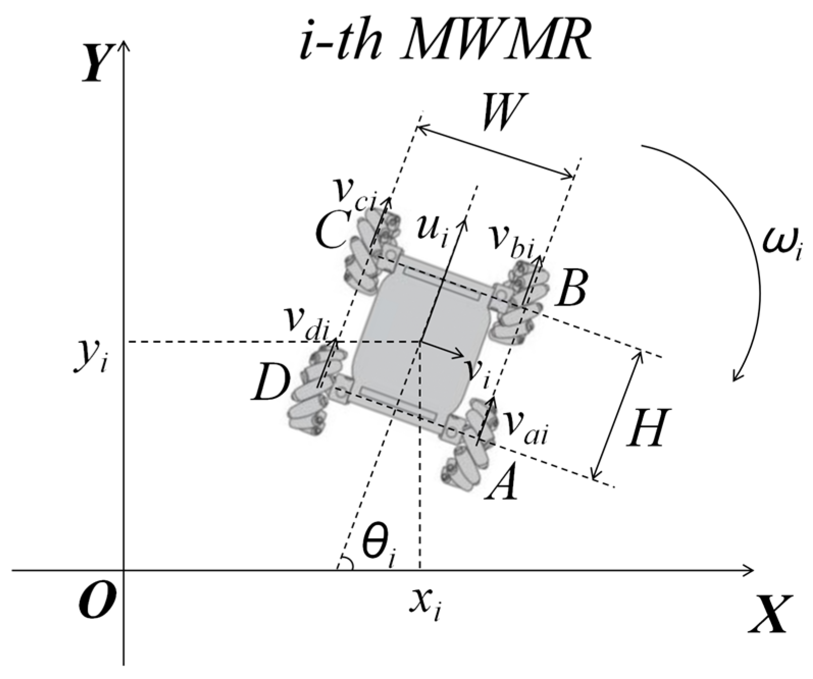
The commonly used WMR models include the two-wheel differential drive model, the Ackermann steering model, and the Mecanum wheel drive model. This paper adopts the Mecanum wheel drive model shown in Figure 1, where A, B, C, and D are denoted as the four driving wheels responsible for providing power to the MWMR. The velocities of the i-th MWMR’s four Mecanum wheels are denoted as , respectively. Let the position of the center of the i-th MWMR in the inertial coordinate system be denoted as . The longitudinal and lateral velocities of the MWMR are and , respectively, while the instantaneous angular velocity is , and the yaw angle of the MWMR is .
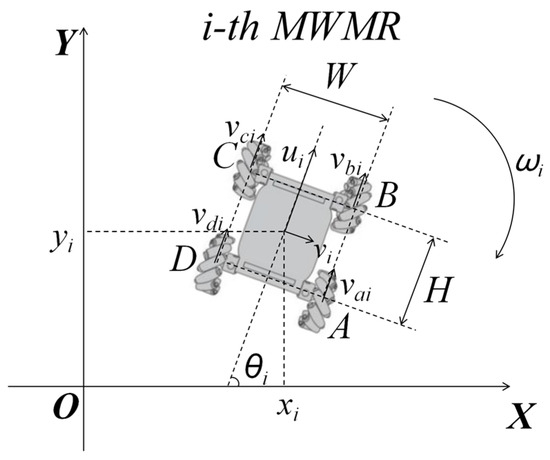
Figure 1.
Mecanum wheel chassis motion model.
Given that the distance between the left and right wheels of the MWMR is , and the distance between the front and rear wheels is , the velocities of the wheels of the i-th MWMR at a certain moment can be expressed as Equation (1):
The longitudinal velocity of the MWMR can be expressed as Equation (2):
The lateral velocity can be expressed as Equation (3):
The angular velocity can be expressed as Equation (4):
In summary, the kinematics of the Mecanum wheel MWMR in the inertial coordinate system can be expressed as Equation (5):
The matrix form of Equation (5) is given by Equation (6):
where denotes the state variables, and denotes the control inputs.
2.2. Kinematic Model Development for Multiple MWMRs Based on the Leader–Follower Method
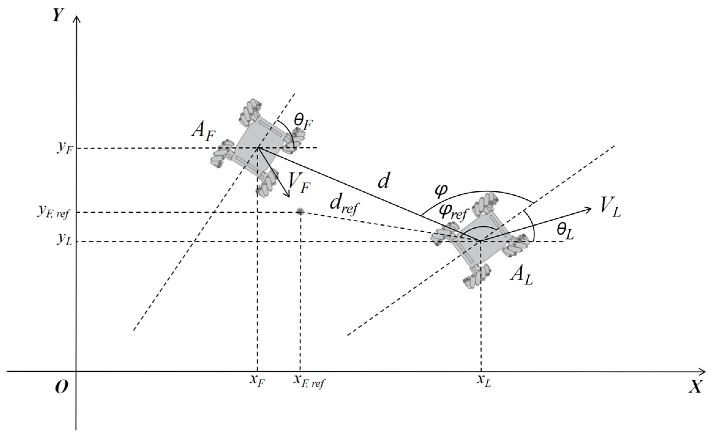
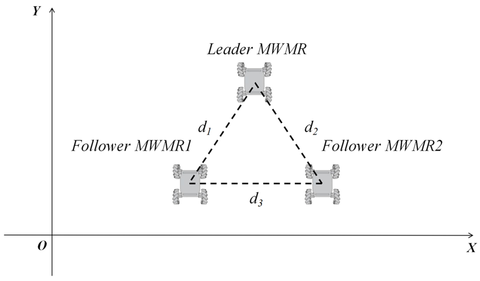
The leader–follower method is widely used in the field of multi-agent formation control due to its advantages, such as reliability and low communication overhead. It meets the requirements for multi-MWMR path planning tasks in uncertain environments, as outlined in this paper. As shown in Figure 2, AL denotes the Leader MWMR, and AF denotes the Follower MWMR. The distance between AL and AF is denoted by , and is the angle between the MWMR’s orientation and the distance . According to the leader–follower method, the desired position of the Follower MWMR AF can be determined from the state variable X of the Leader MWMR AL. During the formation process, the Follower MWMR maintains the formation by adjusting its position according to the desired coordinates. The relationship is given by Equation (7):
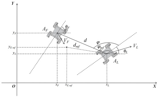
Figure 2.
Schematic diagram of the multi-MWMR model.
The kinematic model of the Follower MWMR is shown in Equation (8):
2.3. Establishment of the Driving Environment Model for MWMRs
The construction of the driving environment model is an essential prerequisite for designing MWMR path planning algorithms. In this study, we use the APF algorithm to build the MWMR’s driving environment model, with a focus on solving the problem of MWMR avoidance of concave obstacles and moving obstacles in uncertain environments. In the APF algorithm, obstacles and the target point generate repulsive and attractive potential fields, denoted as and , respectively. The repulsive potential field repels the MWMR, reaching its maximum value at the position of the obstacle. The attractive potential field attracts the MWMR, reaching its minimum value at the target location. When the MWMR moves within the resultant potential field , which is the combination of both attractive and repulsive fields, it moves from the initial position with higher potential to the target position with lower potential, thus planning a collision-free path from the initial to the target position. The resultant potential field can be expressed by Equation (9):
In this section, given the known initial position and target point, an improved artificial potential field is proposed for the real-time path planning of MWMRs in a two-dimensional complex environment. The elaborate architecture of the potential field model within the context of the driving environment is delineated hereinafter.
2.3.1. Target Point
In the path planning process, it is necessary to obtain a smooth and collision-free path connecting the initial position to the target position. To guide the MWMR toward the target location, the attractive potential field function (10) is used to describe the target position as follows:
where is a parameter of the attractive potential field, which determines the magnitude and shape of the attractive field. denotes the Euclidean distance between the MWMR and the target position. The value of this function decreases as the distance between the MWMR and the target point reduces, ensuring that the MWMR, within the attractive potential field, ultimately reaches the target location.
2.3.2. Uncrossable Obstacle
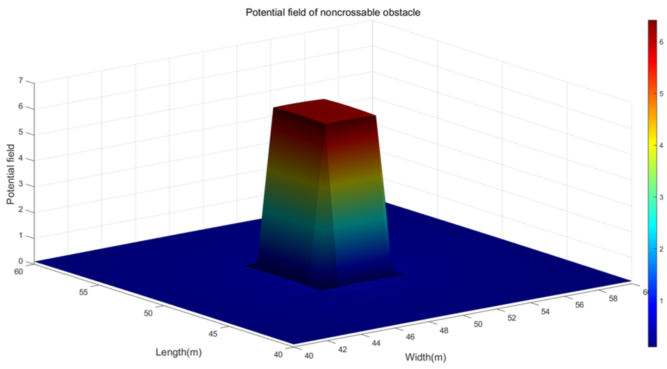
When the MWMR navigates in an uncertain environment, it may encounter uncrossable obstacles, such as rocks, walls, etc. Forcing the MWMR to cross these obstacles could cause damage to the vehicle. The repulsive potential field function for uncrossable obstacles is defined as Equation (11). The model of the repulsive potential field is shown in Figure 3.
where , , and are parameters of the repulsive potential field, which determine the magnitude and shape of the repulsive field. denotes the Euclidean distance between the MWMR and the obstacle. is the maximum detection range of the MWMR’s sensors. is the safety distance between the MWMR and the obstacle, which can be expressed by Equation (12).
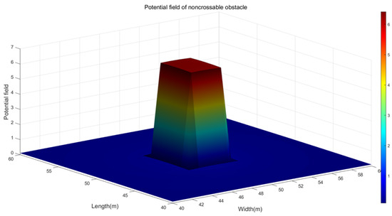
Figure 3.
Repulsive potential field generated by uncrossable obstacles.
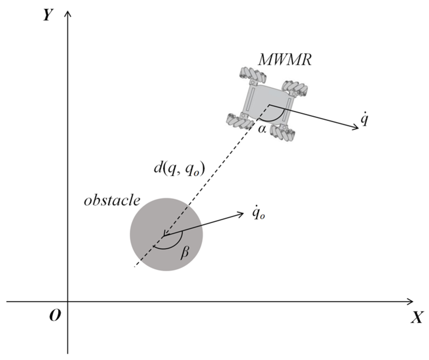
In this context, denotes the minimum safe distance between the MWMR and the obstacle, while is the safe time interval. denotes the velocity of the obstacle, and refers to the velocity of the MWMR. is the angle between the direction of the MWMR’s velocity and the Euclidean distance line connecting the MWMR and the obstacle, denoted as . denotes the angle between the velocity direction of the obstacle and the direction of the Euclidean distance between the MWMR and the obstacle, as shown in Figure 4.

Figure 4.
Schematic diagram of angles and .
For stationary obstacles located far from the target position, the rate of change in the repulsive potential field function denoted by Equation (11) increases as the distance between the MWMR and the obstacle decreases. Ultimately, it tends to infinity, causing the MWMR to move away from the obstacle. For stationary obstacles near the target position, the repulsive potential field function has a global minimum at the target location, which effectively prevents the problem of unreachable targets.
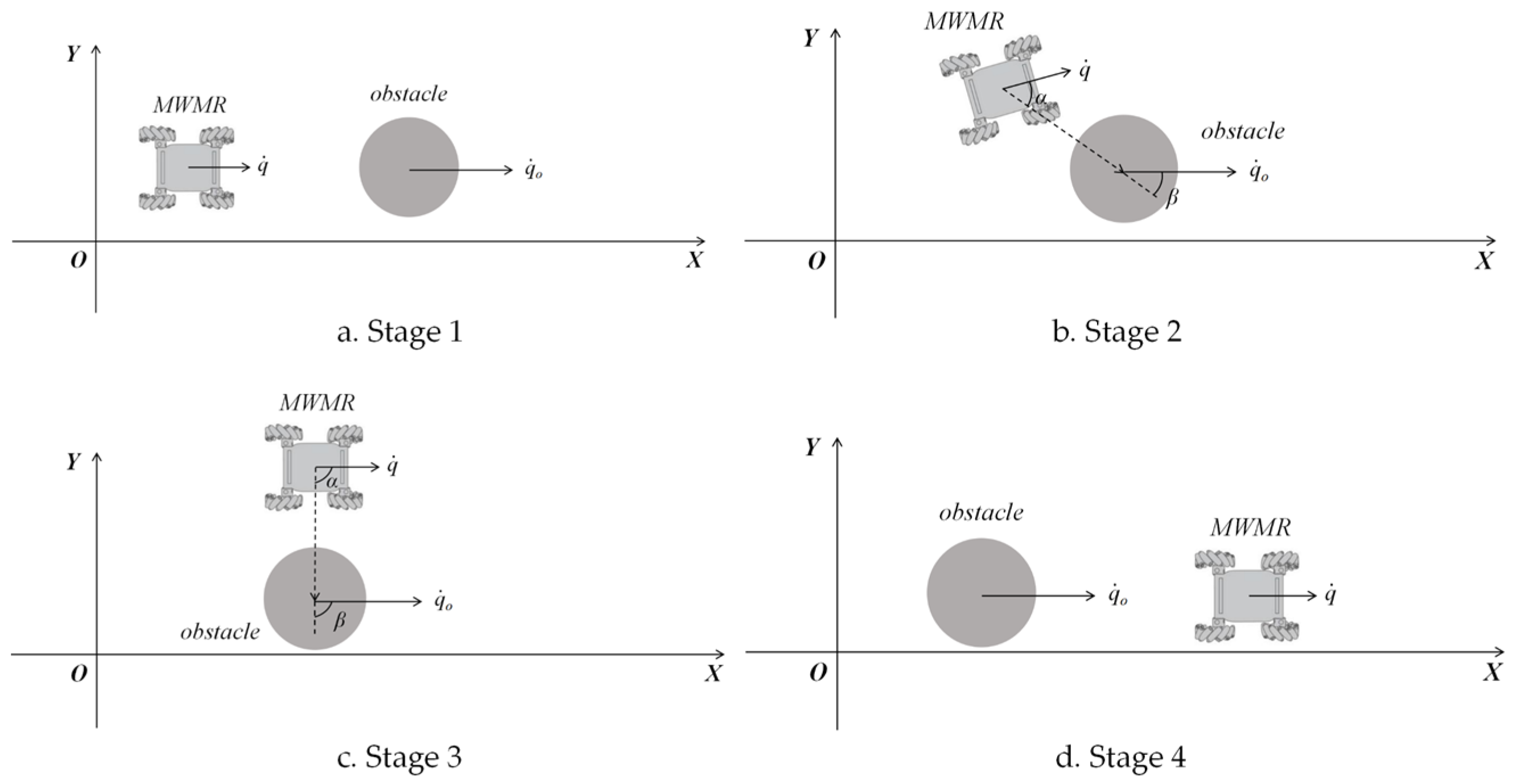
For moving obstacles, the value of the repulsive potential field is influenced by both the relative position and the relative velocity between the MWMR and the obstacle. A typical process for avoiding moving obstacles is shown in Figure 5. As illustrated in Figure 5a, when a moving obstacle appears directly ahead of the MWMR, with , the expression holds. In this case, the value of the repulsive potential field is determined by the distance between the MWMR and the obstacle. The MWMR moves in the direction away from the obstacle. In Figure 5b, when the MWMR begins to bypass the obstacle, it accelerates in the direction where and increase; that is, the MWMR accelerates to move around the obstacle. As shown in Figure 5c, when the movement direction of the MWMR is parallel to that of the obstacle, with , the expression holds. In this situation, the MWMR continues to accelerate in the direction where and increase, thereby bypassing the obstacle. Finally, in Figure 5d, after obstacle avoidance is complete, the obstacle is positioned directly behind the MWMR, with , and the expression holds. The faster the MWMR moves, the lower the probability of collision with the obstacle.
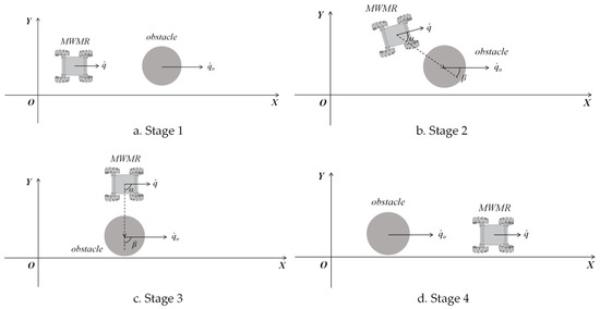
Figure 5.
Process of MWMR avoiding moving obstacles.
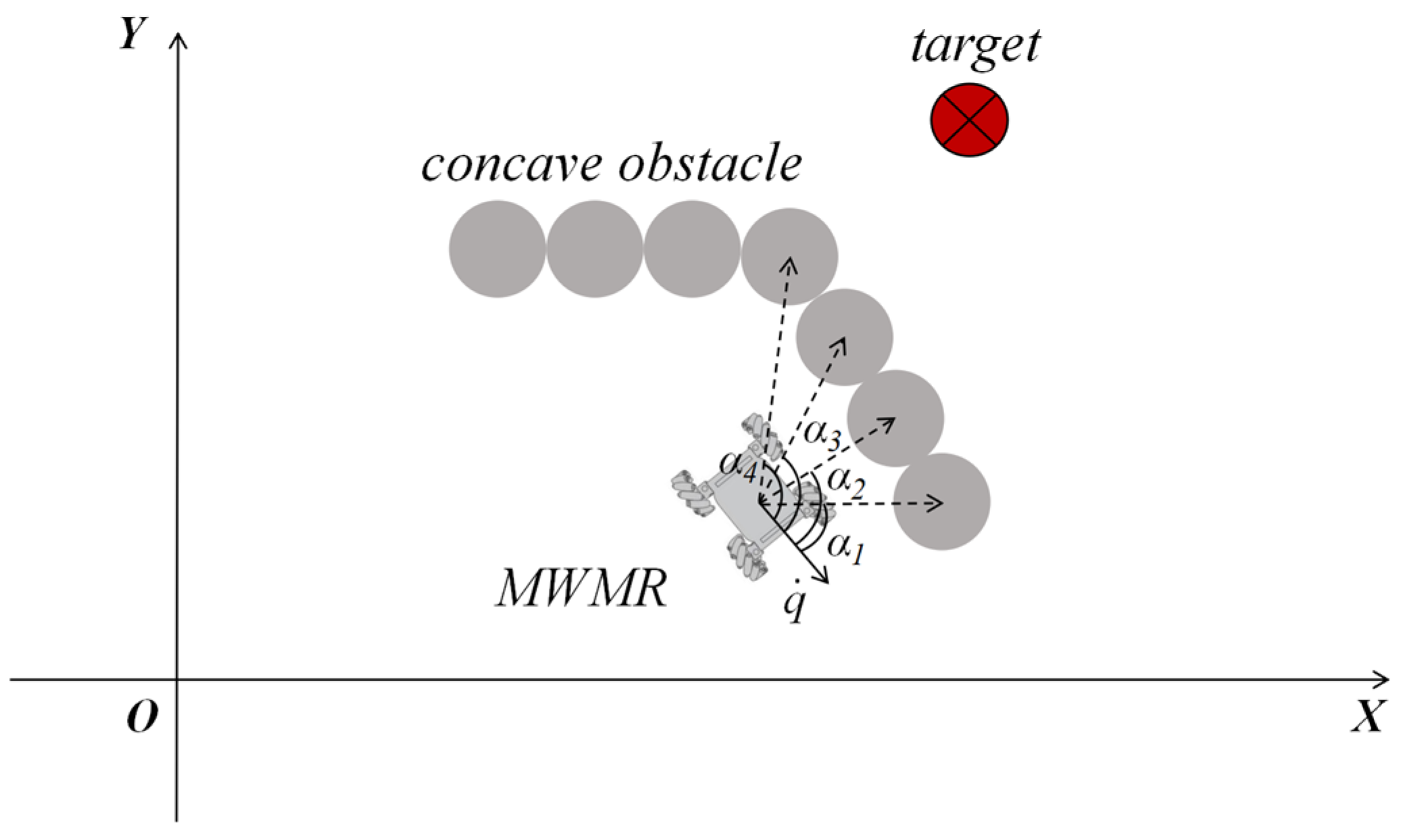
For concave obstacles, as shown in Figure 6, the MWMR will move in the direction where increases. This allows the MWMR to bypass the concave obstacle.

Figure 6.
Schematic diagram of MWMR avoiding concave obstacle.
3. Design of Multi-MWMR Path Planning Algorithm
As MWMR application scenarios become more complex, individual MWMRs face issues such as low efficiency and insufficient capabilities. The increasingly uncertain operating environments and complex task requirements make it inevitable for MWMR systems to evolve towards clustering, autonomy, and intelligence. In this section, we designed a multi-MWMR path planning algorithm. To ensure real-time path planning for multiple MWMRs in uncertain environments, we proposed a path planning controller based on the integration of the artificial potential field and MPC, specifically for the path planning of the Leader MWMR. For the formation control problem in multi-MWMR systems, we proposed a leader–follower method based on the enhanced APF algorithm. The desired positions of the Follower MWMRs were treated as the goal points of the enhanced APF algorithm, as determined by Equation (7). The remaining MWMRs in the formation and the obstacles were treated as obstacles in the enhanced APF algorithm. This approach achieves low computational cost while maintaining the multi-MWMR formation, avoiding complex obstacles, and ensuring collision avoidance within the formation.
3.1. Design of Path Planning Controller for MWMRs
In this section, we first linearized and discretized the kinematic model of the MWMR presented in Section 2 to obtain the prediction model. Next, we designed the objective function for the MWMR path planning problem, incorporating both repulsive and attractive potential fields into the objective. We then proposed an optimal path planning controller that comprehensively considers the MWMR’s kinematics and the driving environment.
The MPC algorithm is capable of predicting the MWMR’s response over the next time steps. Based on these predictions, it optimizes factors such as MWMR kinematics and obstacle avoidance, thereby generating an optimal control sequence for the following time steps. To obtain a collision-free path for the MWMR, we designed an objective function for path planning based on the prediction model, which is delineated hereinafter.
3.1.1. Linearization and Discretization of the Kinematic Model
Based on the kinematic model of the MWMR (Equation (6)), the kinematic model can be reformulated as Equation (13):
where denotes the system output, and is the output matrix of the system.
We assume that, at time t, there is a small error between the current position and the desired position . The state Equation (13) at can be expanded using a Taylor series, neglecting the quadratic and higher-order terms. This yields Equation (14):
In this case, and are the partial derivative matrices of the state Equation (11) with respect to the system state variables and input variables, respectively. They can be expressed as Equation (15):
Next, we discretize the state Equation (14) using the Euler method. Let the sampling time be denoted as T. The discrete form is then obtained, as shown in Equation (16):
where
To further eliminate the steady-state error, we augment the system variables by incorporating the control input and state variable , resulting in a new state variable . Therefore, the predictive model can be expressed as Equation (18):
where , , , .
Based on the prediction model in Equation (18), we can derive a predictive equation to forecast the output over a future time horizon. The predictive equation can be expressed as Equation (19).
where
where denotes the prediction horizon, and denotes the control horizon. Typically, .
3.1.2. Design of the Objective Function for the MPC Path Planning Controller
To generate a smooth, collision-free path for the MWMR, it is necessary to design a reasonable objective function and apply the optimal control increment to the MWMR model. This objective function should be based on the driving environment established in Section 2, ensuring that the output remains as close as possible to the desired value. At the same time, to suppress abrupt changes in the input, it is essential to constrain the magnitude of the control increment. Therefore, we have designed the following objective function:
The specific objective function can be expressed as Equation (21):
In this equation, , , and are positive definite and symmetric weighting matrices, and denotes the predicted value at the i-th step in the future, given the current time step k. The objective function consists of three components: tracking, input variation, and the potential field of the predicted driving environment. The first component aims to ensure that the output tracks the predefined predicted values. The second component provides a soft constraint on the control increment to suppress abrupt changes in control inputs. The third component ensures that the MWMR generates a collision-free path.
3.2. Design of a Formation Controller for Multiple MWMRs
In the multi-MWMR path planning process based on the fusion of the artificial potential field and MPC, the Leader MWMR moves toward the target point solely under the influence of the path planning controller, without considering the Follower MWMRs in the formation. The Follower MWMRs, under the influence of the formation controller, maintain the formation and avoid obstacles and other MWMRs in the formation based on the desired positions obtained from Equation (7). The specific details are given in Algorithm 1. Considering the relative velocities between the Follower MWMRs, obstacles, and the target point, we propose an enhanced APF algorithm for the Follower MWMRs to maintain the formation in real-time and avoid obstacles, which reduces the computational burden. In the enhanced APF algorithm, the desired position of the Follower MWMRs is treated as an attractive target point to ensure the formation, while other MWMRs within the formation and external obstacles are treated as repulsive entities to avoid collisions within the formation and obstacles outside it.
| Algorithm 1: Expected Position Generation Function. |
| Input: The current moment k, current State Variables of Leader UGV at time k + 1, the quantity n of Follower UGVs, the expected distance di,ref between the Leader UGV and i-th Follower UGV, the expected angle between the Leader UGV and the i-th Follower UGV. |
| Output: Expected Position of Follower UGV . 1: For each Follower UGV j (j < n) 2: The expected position of the j-th Follower UGV on the X-axis at time k + 1. 3: The expected position of the j-th Follower UGV on the Y-axis at time k + 1. 4: End for 5: Return . |
3.2.1. Attraction Force Optimization Based on the Enhanced APF Algorithm
The traditional APF algorithm only considers the relative distance between the MWMR and the target point for attraction force, which is not suitable for uncertain environments and frequently moving target points. In the case of the expected position that continuously moves with the Leader MWMR, we take into account the relative velocity between the Follower MWMRs and the target position in the enhanced APF algorithm. Additionally, to limit the maximum velocity of the Follower MWMRs, we introduce the concept of desired velocity. Based on these considerations, we derive the expression for the total attraction force , which includes the distance attraction force , the velocity attraction force , and the desired velocity attraction force , as shown in Equation (22):
- (1)
- Modeling of Distance Attraction Force
The distance attraction force ensures that the MWMR moves towards the target. The distance attraction potential field function is given by Equation (23):
where is the positive proportional coefficient, denotes the position of the i-th Follower MWMR, and is the desired position of the i-th Follower MWMR.
The distance attraction force is defined as the negative gradient of the distance attraction potential field , as shown in Equation (24):
- (2)
- Modeling of Velocity Attraction Force
The velocity attraction force enhances the adaptability of the MWMR to moving targets. The velocity attraction potential field function is given by Equation (25):
where is the positive proportional coefficient.
The velocity attraction force is defined as the negative gradient of the velocity attraction potential field , as shown in Equation (26):
- (3)
- Modeling of Desired Velocity Attraction Force
The desired velocity attraction force ensures that the MWMR can move at a predefined desired velocity. The desired velocity attraction potential field function is given by Equation (27):
where is the positive proportional coefficient, and denotes the desired velocity of the i-th Follower MWMR.
The desired velocity attraction force is defined as the negative gradient of the desired velocity attraction potential field , as shown in Equation (28):
3.2.2. Repulsion Force Optimization Based on the Enhanced APF Algorithm
The traditional APF algorithm considers only the relative distance between the MWMR and obstacles for repulsion force. However, it is not suitable for uncertain environments that include moving and concave obstacles. In the enhanced APF algorithm, we further account for the relative velocity between the Follower MWMRs and the obstacles. This leads to the expression for the repulsion force , as shown in Equation (29):
where denotes the distance repulsion force, and denotes the velocity repulsion force.
- (1)
- Modeling of Distance Repulsion Force
To address the unreachable goal issue of the traditional APF algorithm, we propose a distance repulsion potential field , where the repulsive potential at the target point is zero. The detailed formulation is given in Equation (30):
where is the proportional coefficient. and denote the external obstacles relative to the formation and the j-th MWMR () within the formation, respectively. For external obstacles, . denotes the maximum collision-avoidance distance between MWMRs within the formation, where .
The repulsive force is the negative gradient of , as shown in Equation (31):
- (2)
- Modeling of Velocity Repulsive Force
For moving obstacles in an uncertain environment, we consider the relative velocity between the MWMR and the obstacles. A velocity repulsive potential field, as shown in Equation (32), is proposed. This field accounts for the dynamic interaction between the MWMR and the moving obstacles.
where is the proportional coefficient, and denotes the angle between the relative velocity and the relative position of the MWMR and the obstacle, as shown in Figure 7.
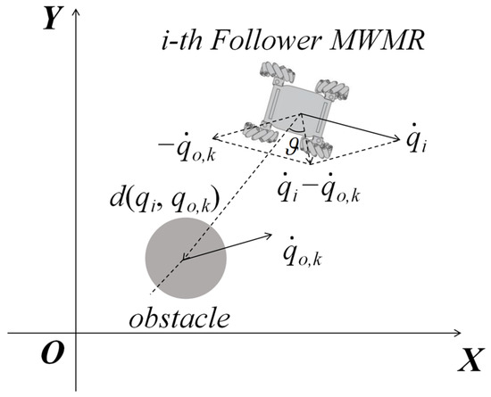
Figure 7.
Schematic diagram of angle .
The velocity repulsive force is the negative gradient of , as shown in Equation (33):
4. Simulation and Experiment
In this section, we validate the effectiveness of the proposed path planning algorithm and formation control algorithm in uncertain environments through both simulation and real-world experiments. First, we set up two different simulation scenarios to compare the proposed method with the APF-MPC algorithm [35], in order to verify the effectiveness and superiority of the proposed path planning algorithm. Among them, Scenario 1 is designed to test the performance of the algorithm in a simple environment with only static obstacles. Scenario 2 is used to evaluate the algorithm’s performance in a complex environment with moving and concave-shaped obstacles. The simulations are conducted on a computer with the following hardware: Intel(R) Core(TM) i5-12400F, 2.50 GHz, and 32 GB RAM. In addition, we apply the proposed path planning algorithm to the path planning of a Mecanum wheel robot, to demonstrate the practical applicability and effectiveness of the algorithm in real-world applications.
4.1. Simulation Result
For an MWMR, common task environments can be classified into simple and complex environments based on the level of complexity. In simple environments, obstacles are sparsely distributed, while, in complex environments, obstacles are densely arranged and may include hard-to-avoid concave obstacles. In this study, we select both simple and complex environments as simulation scenarios and use the APF-MPC algorithm as the comparison method. The size of the simulation scenarios is 100 m × 100 m for both cases. The performance evaluation metrics for the simulations include path length, path smoothness, longitudinal distance, velocity, and angular velocity. The detailed initial parameters for the simulation are provided in Table 1.

Table 1.
Initial parameters for the simulation.
The formation of multiple MWMRs is set as shown in Figure 8. The three MWMRs are positioned at the vertices of an equilateral triangle, with the desired distance between each MWMR set to .

Figure 8.
Formation of multiple MWMRs.
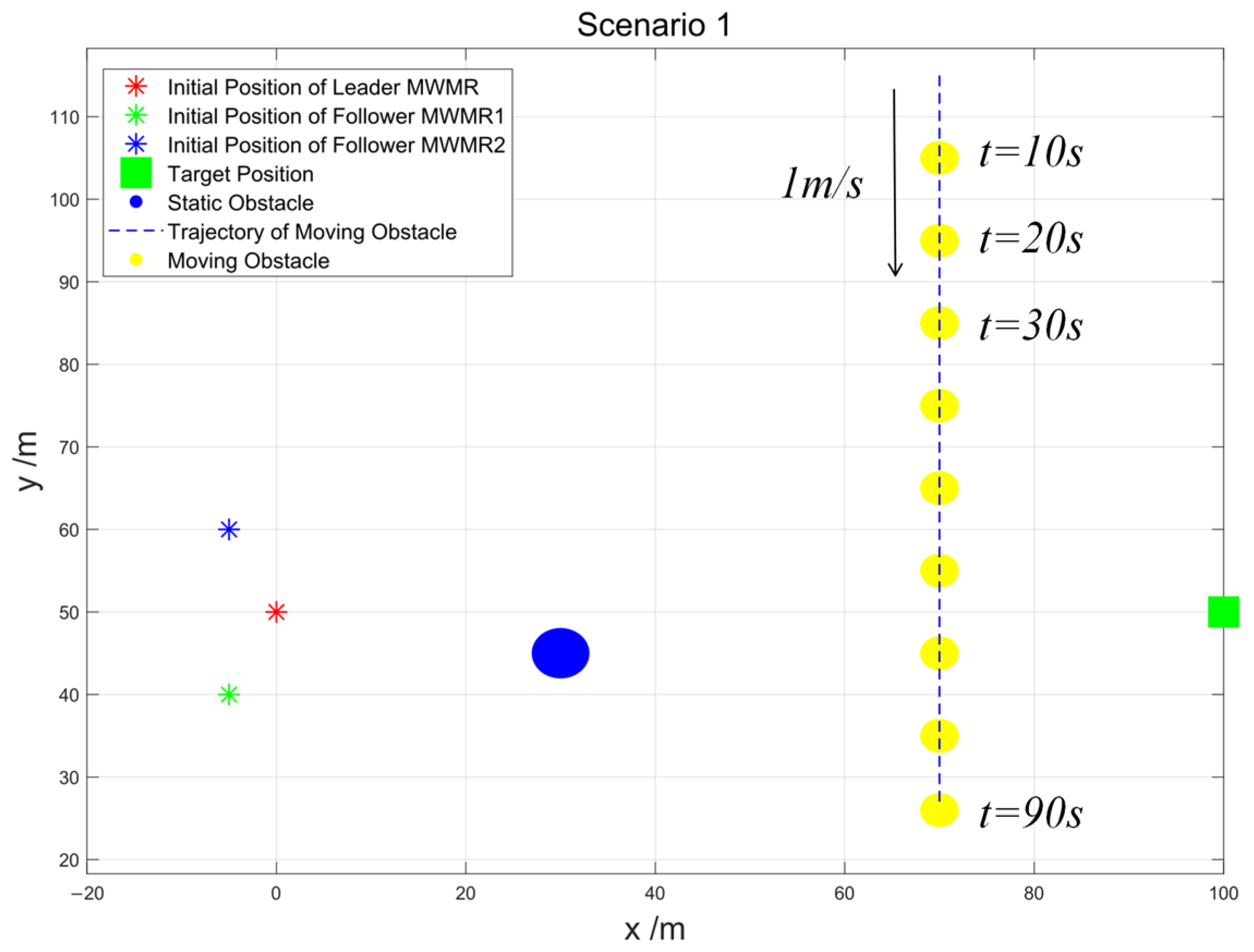
Scenario 1: To verify the effectiveness of the algorithm proposed in this paper in simple environments, we set up the simple scenario shown in Figure 9. The Leader MWMR starts at the initial position (0, 50) and moves towards the target position (100, 50) while avoiding static obstacles. Additionally, it must also avoid a moving obstacle, which starts at position (70, 115) and moves with a speed of = 1 m/s in the negative Y-axis direction.

Figure 9.
Scenario 1.
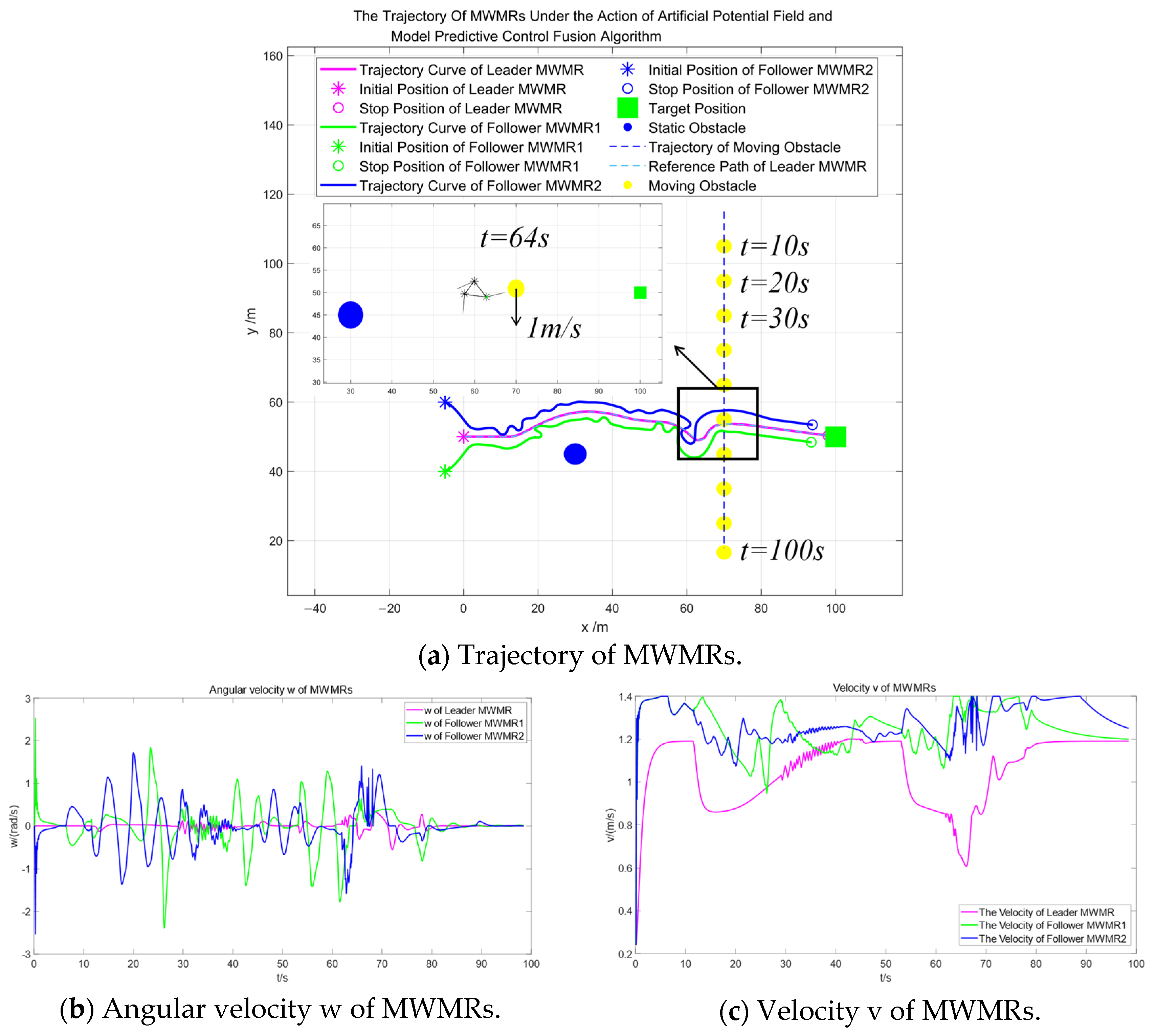
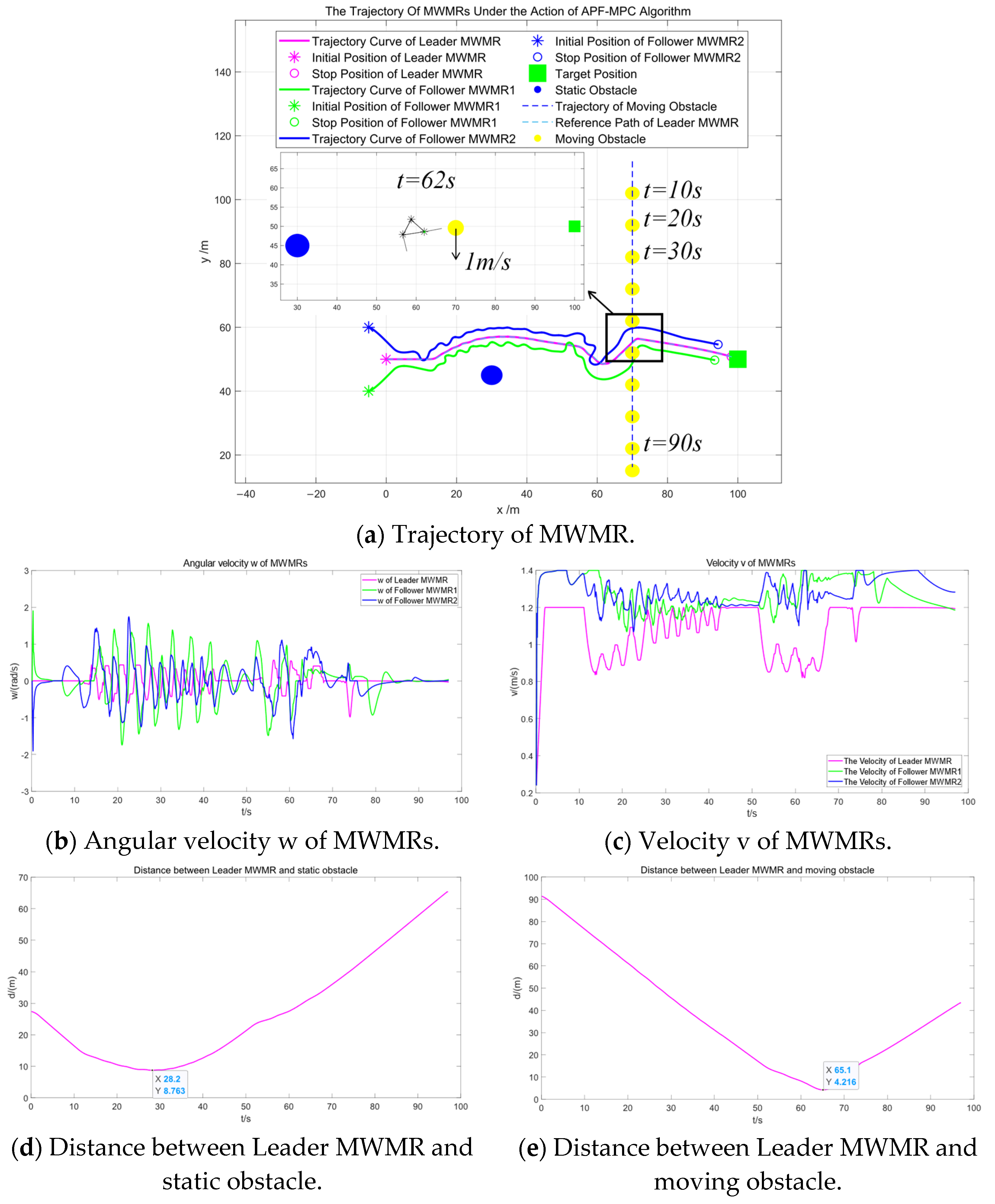
Figure 10a shows the trajectories of multiple MWMRs under the action of the artificial potential field and the model predictive control fusion algorithm. The red curve represents the trajectory of the Leader MWMR, while the blue and green curves represent the trajectories of the Follower MWMRs. Figure 10b,c illustrates the angular velocities and velocities of the multiple MWMRs. It can be observed that the fluctuations of both quantities remain within normal ranges.
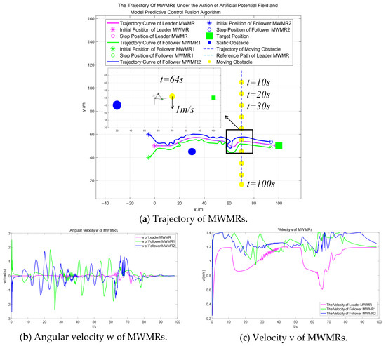
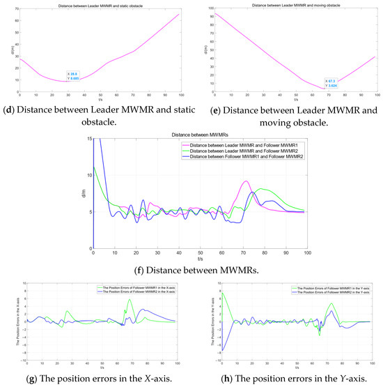
Figure 10.
Simulation results under the artificial potential field and model predictive control fusion algorithm in Scenario 1.
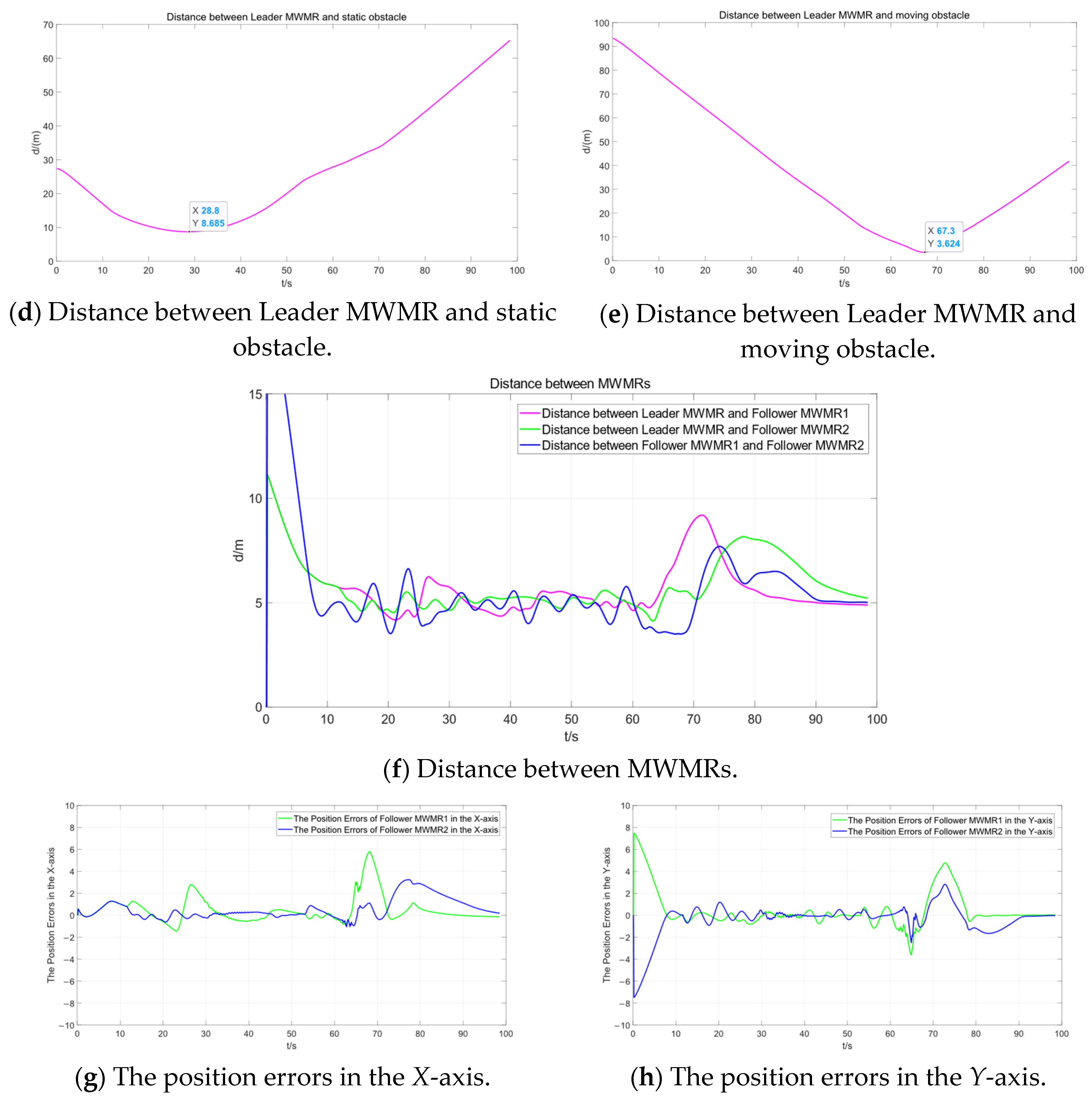
Figure 10d represents the distance between the Leader MWMR and a static obstacle. It can be observed that, under the proposed algorithm, the multi-MWMR system is able to safely avoid static obstacles. The minimum distance between the Leader MWMR and the static obstacle is 8.7 m. At t = 64 s, the multi-MWMR system begins to avoid a moving obstacle. From Figure 10a–c, it is clear that the Leader MWMR first decelerates in the negative direction of the Y-axis. Subsequently, under the influence of the potential field model proposed in this paper, it moves in the positive direction of the Y-axis to avoid the advancing direction of the moving obstacle. Figure 10e represents the distance between the Leader MWMR and the moving obstacle, showing that the minimum distance between them is 3.6 m.
Figure 10f represents the distance between the three MWMRs in the formation. Figure 10g,h represents the errors in the X-axis and Y-axis, respectively, between the Follower MWMRs and the desired positions. From Figure 10f–h, it can be observed that the distances between the MWMRs remain within a normal range and converge after avoiding moving obstacles.
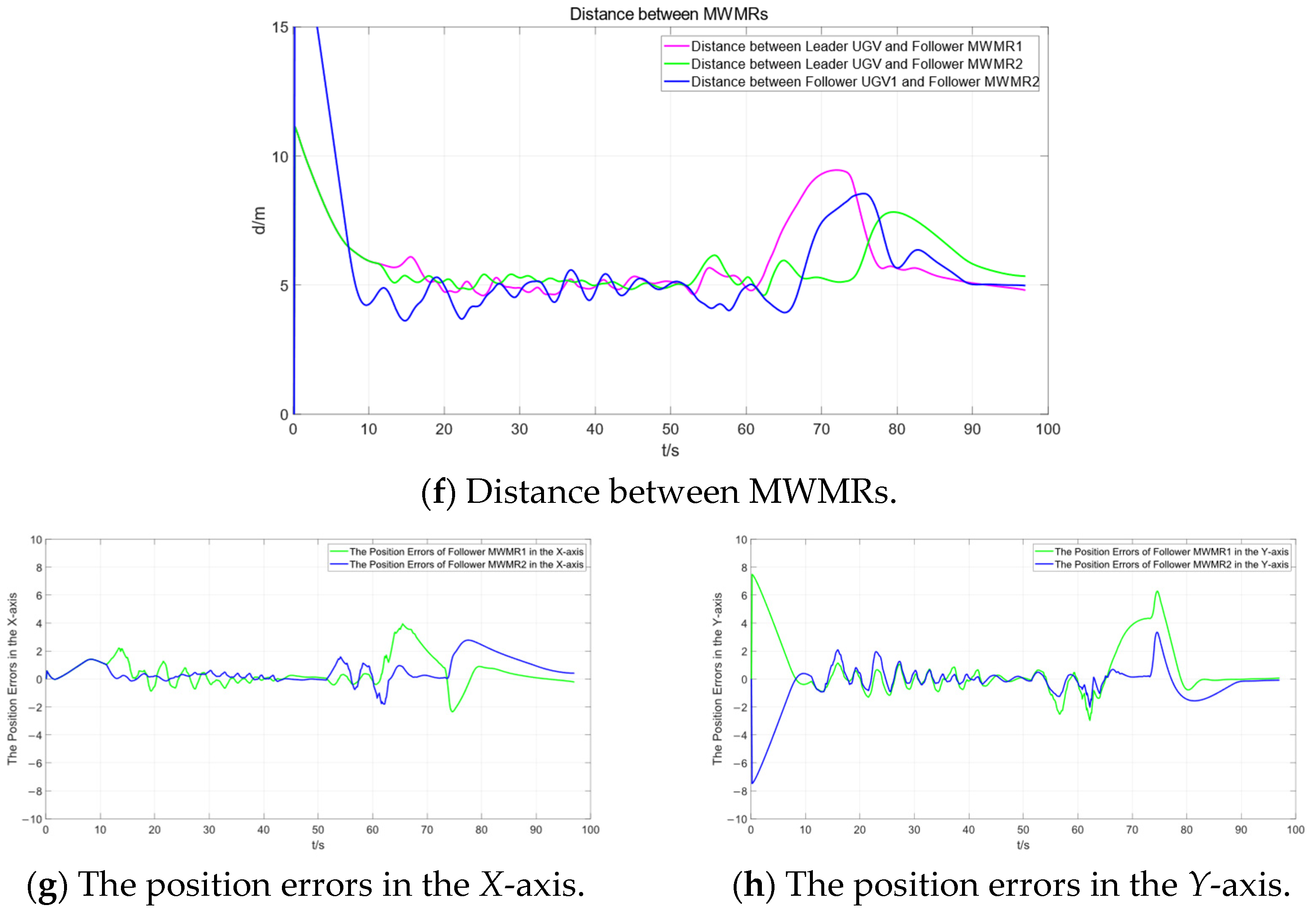
Figure 11 shows the simulation results of multiple MWMRs in Scenario 1 under the APF-MPC algorithm. By comparing Figure 10 and Figure 11, it can be observed that both the artificial potential field and MPC fusion algorithm and the APF-MPC algorithm are able to smoothly avoid static obstacles and safely navigate around moving obstacles. Comparing Figure 10b,c with Figure 11b,c, it is evident that the Leader MWMR under the artificial potential field and MPC fusion algorithm avoids obstacles more smoothly than under the APF-MPC algorithm.
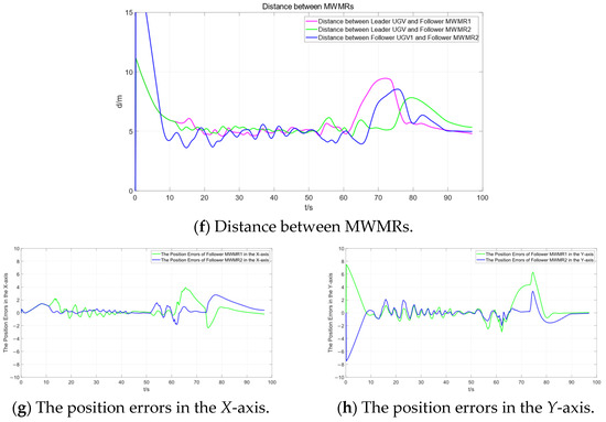
Figure 11.
Simulation results under the APF-MPC algorithm in Scenario 1.
To compare the performance of different path planning algorithms, we established a metric to evaluate the smoothness of the path, as described in reference [36]. As shown in Equation (34), N denotes the total number of path points, and denotes the coordinates of the i-th path point.
Based on the multi-MWMR path planning simulation experiments in the simple environment described above, the evaluation metrics such as path length, simulation duration, and the path smoothness of the Leader MWMR are obtained, as shown in Table 2.
Table 2.
Evaluation metrics.
The results show that, in Scenario 1, under the influence of the artificial potential field and MPC fusion algorithm, the path length of the Leader MWMR is reduced by 2.19% compared to the APF-MPC algorithm. Additionally, the simulation time is reduced by 59.82%, and the path smoothness is smaller, indicating a smoother path. In summary, in a simple environment, the artificial potential field and MPC fusion algorithm improves the stability and feasibility of MWMR path planning compared to the APF-MPC algorithm. It also further enhances the smoothness of the path and reduces the computational burden. Furthermore, the above experiment also validates the effectiveness of the formation control method based on the enhanced APF algorithm and leader–follower method in Scenario 1.
Scenario 2: To validate the effectiveness of the proposed algorithm in complex environments, we set up a complex scenario as shown in Figure 12. The Leader MWMR moves from the initial position (0, 50) to the target position (100, 50), bypassing static obstacles and avoiding a group of three moving obstacles that are moving at 1 m/s in the negative Y-axis direction. Ultimately, the MWMR avoids obstacles near the target position and reaches the target point.
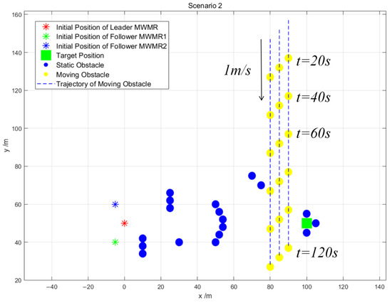
Figure 12.
Scenario 2.
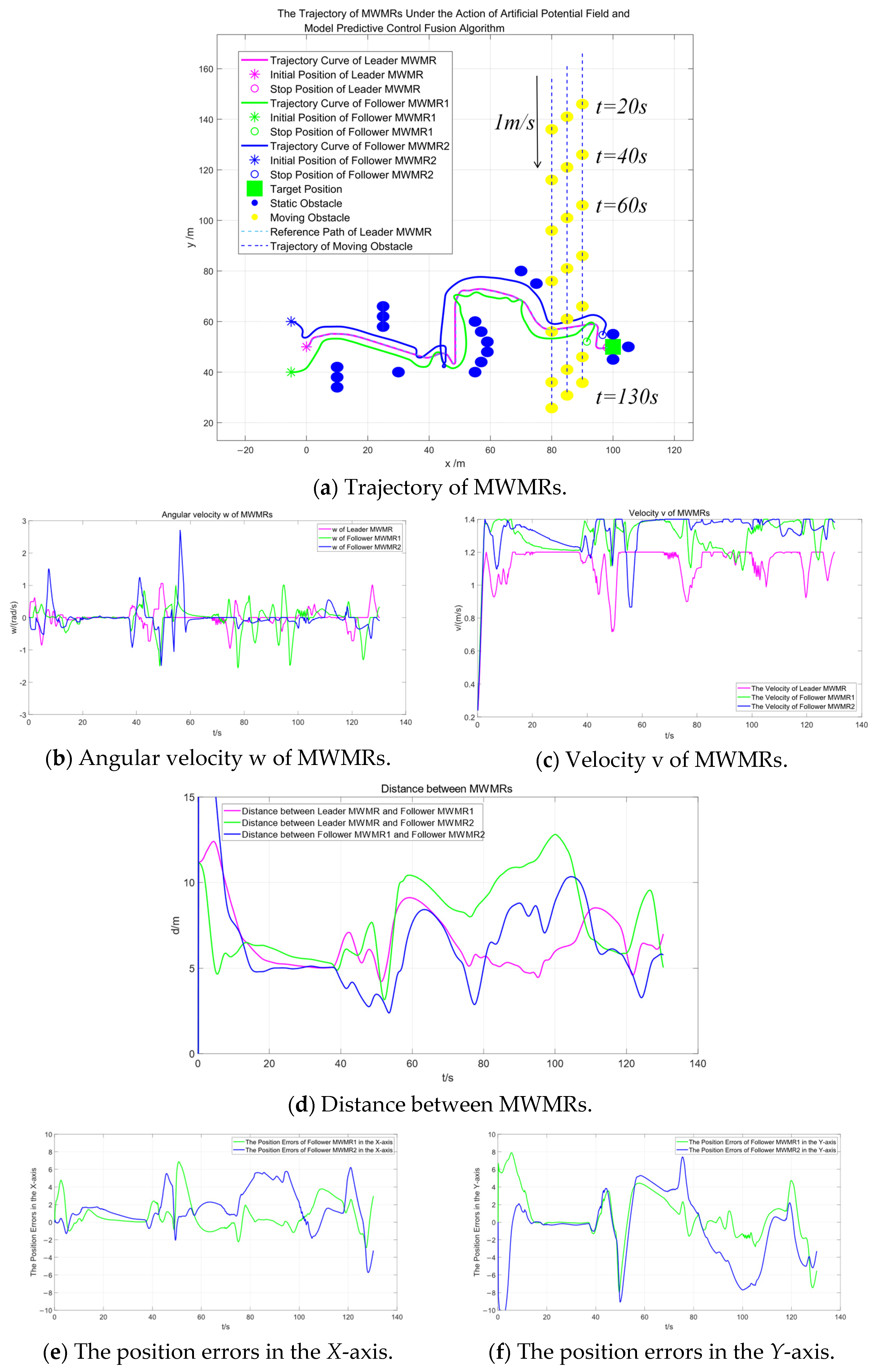
Figure 13a shows the trajectories of multiple MWMRs under the influence of the artificial potential field and model predictive control fusion algorithm. The red curve represents the trajectory of the Leader MWMR, while the blue and green curves represent the trajectories of the Follower MWMRs. Figure 13b,c displays the angular velocity and linear velocity of the multiple MWMRs, respectively. It can be observed that the fluctuations of both velocities remain within a normal range.
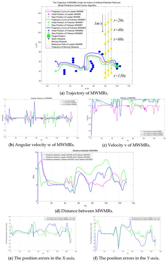
Figure 13.
Simulation results under the influence of the artificial potential field and model predictive control fusion algorithm in Scenario 2.
Figure 13a shows that, under the proposed algorithm, multiple MWMRs are able to safely reach the target location in the complex environment of Scenario 2. Between t = 35 s and t = 60 s, the MWMRs use the proposed potential field model to safely avoid a concave obstacle. From t = 75 s to t = 115 s, the MWMRs successfully avoid a group of three moving obstacles. At t = 120 s, the MWMRs, influenced by the attractive potential field in the model, safely avoid a static obstacle near the target location and reach the goal point.
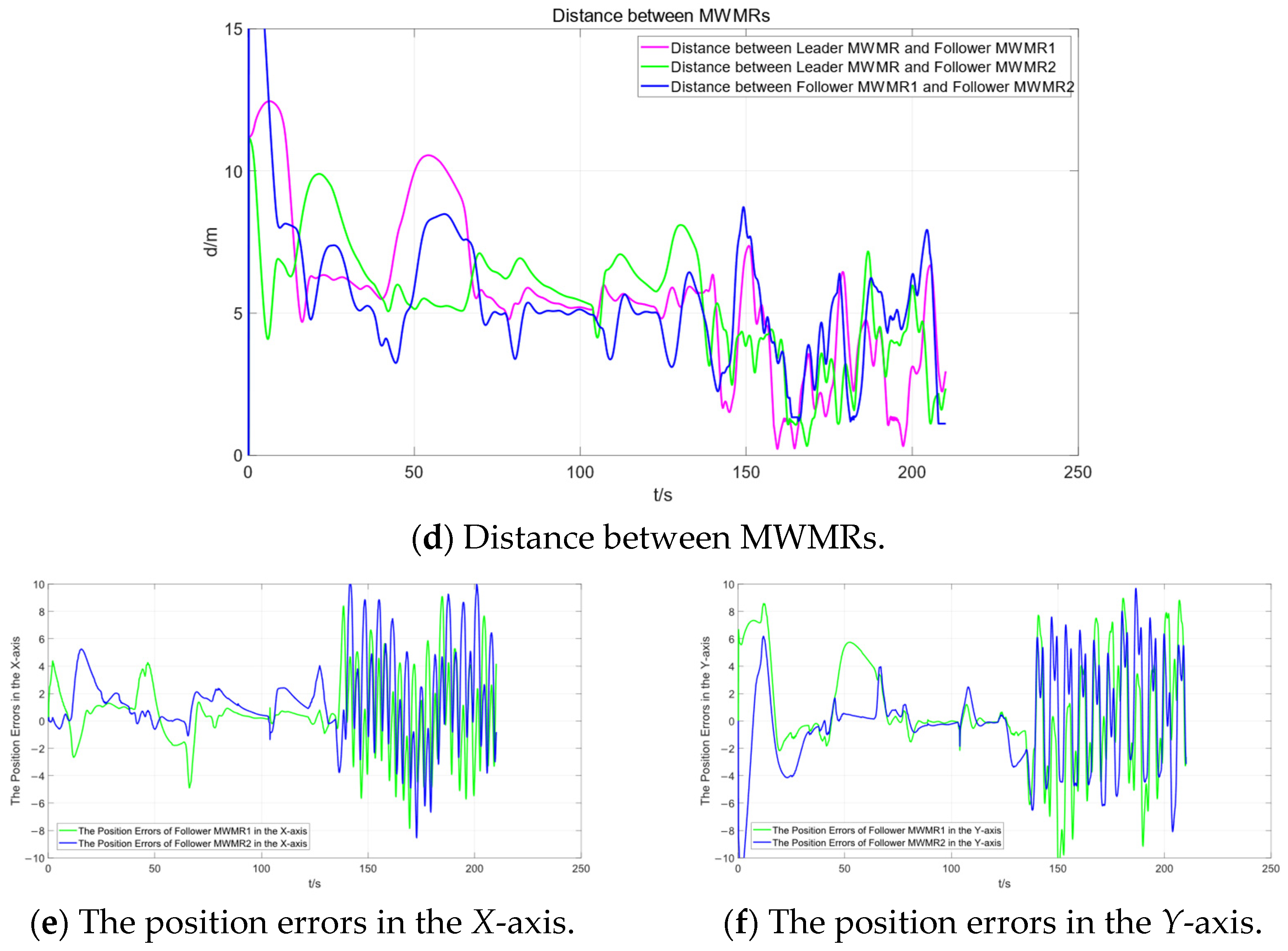
Figure 13d represents the distances between the three MWMRs in the formation. Figure 13e,f shows the errors in the X and Y axes, respectively, between the Follower MWMRs and their desired positions. From Figure 13d–f, it can be observed that, in the complex environment of Scenario 2, the distances between the MWMRs fluctuate as a result of avoiding dense obstacles. However, these distances remain within the normal range.
Figure 14 shows the simulation results of the MWMR formation under the APF-MPC algorithm in Scenario 2. By comparing Figure 13 and Figure 14, it can be observed that both the artificial potential field and MPC fusion algorithm and the APF-MPC algorithm are capable of smoothly avoiding static and moving obstacles. However, as shown in Figure 14a, the multiple MWMRs do not reach the target location. Instead, the multi-MWMR is influenced by obstacles near the target and perform oscillatory motion in the vicinity of the target. From the above simulation results, it can be concluded that the artificial potential field and MPC fusion algorithm proposed in this paper address the unreachable target problem that the APF-MPC algorithm cannot resolve. The proposed algorithm demonstrates better feasibility and stability in complex environments. Additionally, it further validates the effectiveness of the enhanced APF algorithm and the leader–follower method in complex environments.
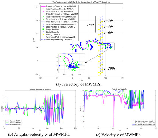
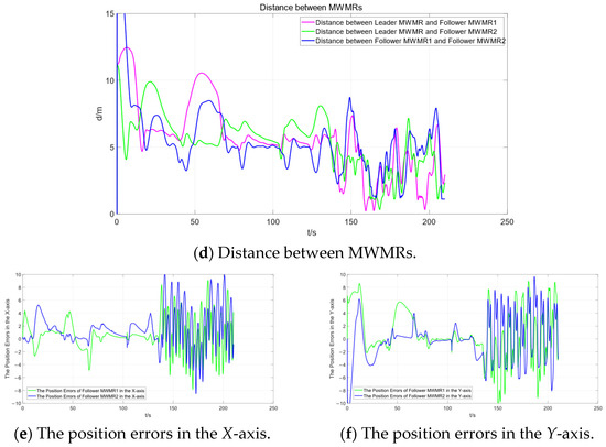
Figure 14.
Simulation Results under the influence of the APF-MPC algorithm in Scenario 2.
4.2. Real-World Experiment
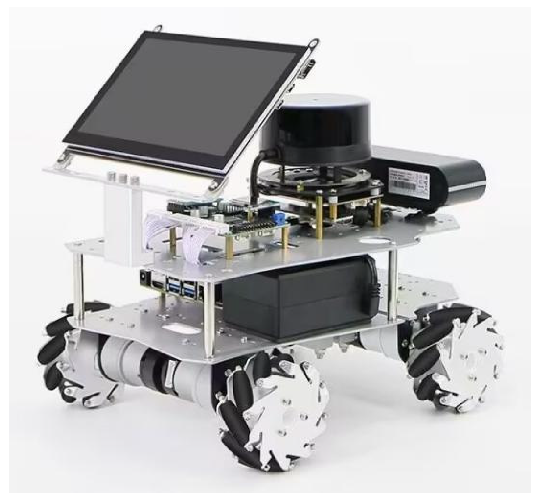
To further validate the effectiveness of the MWMR path planning algorithm based on the fusion of the artificial potential field and MPC, we conducted two sets of real-world experiments using a robot with Mecanum wheels. The experiments were carried out in both simple and complex environments. The robot is shown in Figure 15. The robot was outfitted with an LSLIDAR N10P LiDAR sensor for perception and detection, a Raspberry Pi 4B for data processing, and an STM32 MCU for controlling the Mecanum wheel chassis.
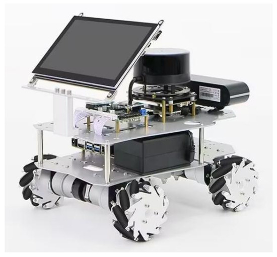
Figure 15.
Mecanum-wheeled mobile robot.
- (1)
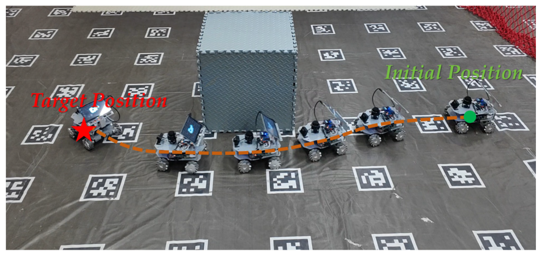
- Simple environment:
In this experiment, there is only one obstacle. The experimental results are shown in Figure 16. This experiment validates the effectiveness of the proposed fusion of the artificial potential field and MPC for practical applications in simple scenarios.
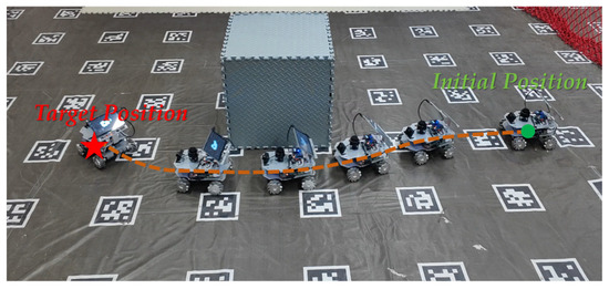
Figure 16.
Experimental results in a simple driving environment.
- (2)
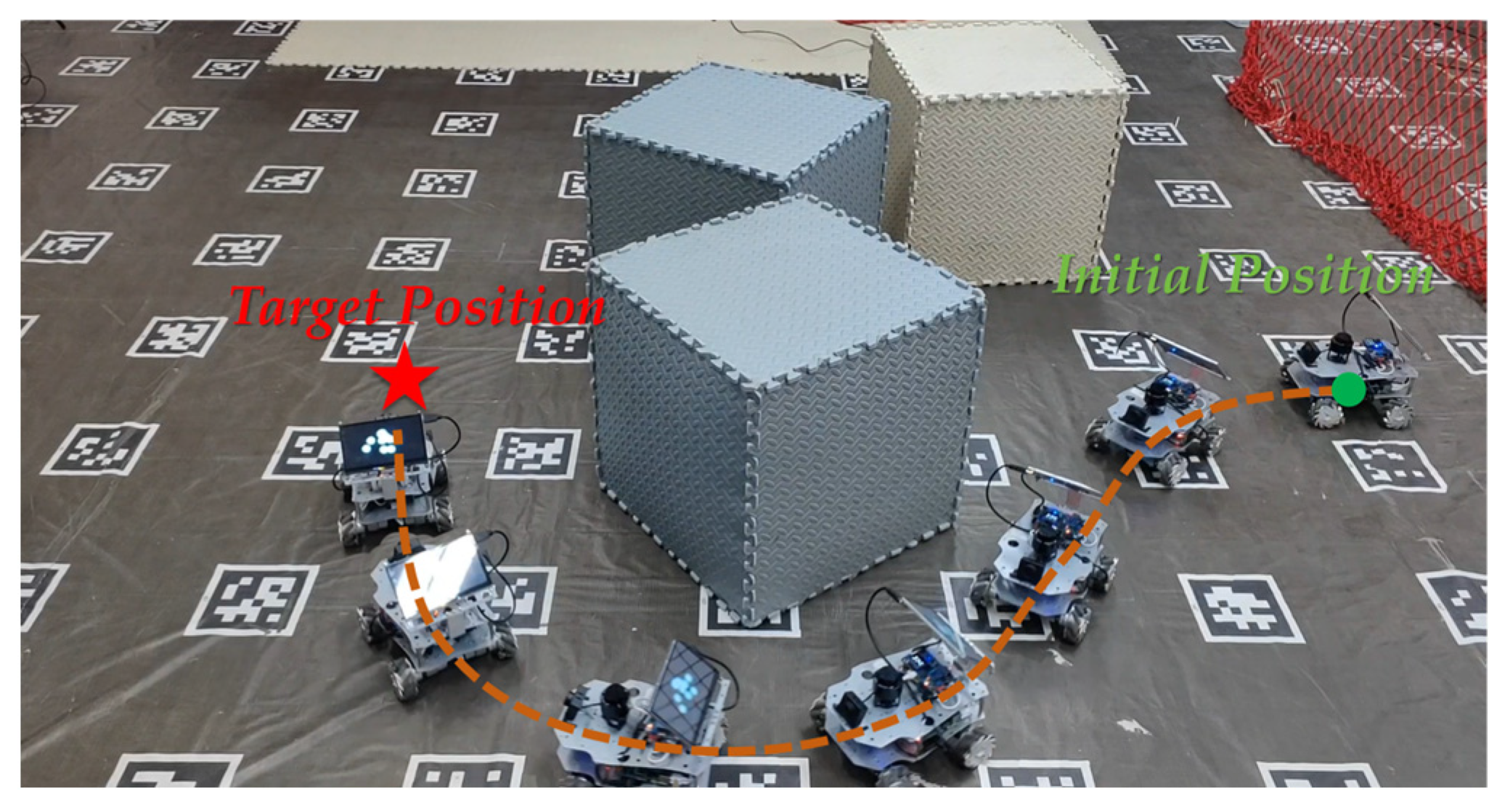
- Complex environment:
In this experiment, there is a concave obstacle composed of three obstacle blocks. The experimental results are shown in Figure 17. This experiment validates the effectiveness of the proposed fusion of the artificial potential field and MPC for practical applications in complex scenarios.

Figure 17.
Experimental results in a complex driving environment.
5. Conclusions
This paper addresses the multi-MWMR path planning and formation control problem in uncertain environments by proposing a fusion algorithm based on the artificial potential field and MPC. The algorithm represents environmental constraints as a potential field model for uncertain environments, integrating both the repulsive potential fields generated by obstacles and the attractive potential fields generated by the target location, which can effectively avoid the issue of local minima. This innovative potential field model is incorporated into the objective function of the MPC path planning controller to obtain a smooth, collision-free trajectory that adheres to the kinematic constraints of the MWMR. Furthermore, a formation control method based on an enhanced APF algorithm and a leader–follower approach is proposed. This method achieves low computational cost formation maintenance, intra-formation collision avoidance, and obstacle avoidance for MWMR formations. The proposed enhanced APF algorithm takes the relative velocities between Follower MWMRs, the target point, and obstacles into account, enabling the stable tracking of moving target points and the safe avoidance of moving obstacles, thus improving the control performance of the multi-MWMR system in uncertain environments. Finally, the simulation results from a simple scenario with only one static obstacle and one moving obstacle, and a complex scenario with concave obstacles and three moving obstacles have verified the stable avoidance capabilities of the method proposed in this paper against static obstacles, moving obstacles, and concave obstacles. Compared to the APF-MPC algorithm, in the simple scenario, the path length of the Leader MWMR under our proposed algorithm decreased by 2.19%, the simulation time was reduced by 59.82%, and the path smoothness was lower, resulting in a smoother path. Furthermore, in the complex environment, our algorithm safely avoided concave obstacles that the APF-MPC algorithm could not. Moreover, the effectiveness of the proposed method in practical applications is further validated through two sets of real experiments. These experiments were conducted in both simple and complex environments. In the future, we will focus on investigating the impact of nonlinear MWMR dynamics on the performance of the path planning algorithm and the interference with formation communications in an uncertain environment and further implement this in real experimental settings.
Author Contributions
Conceptualization, Y.S. and C.S.; methodology, Y.S.; software, Y.S.; validation, Y.S., C.S. and Z.S.; formal analysis, C.S.; investigation, Y.S.; resources, B.L.; data curation, Y.S.; writing—original draft preparation, Y.S.; writing—review and editing, C.S.; visualization, Z.S.; supervision, B.L.; project administration, B.L.; funding acquisition, B.L. All authors have read and agreed to the published version of the manuscript.
Funding
This project is supported by the National Nature Science Foundation of China, Grant/Award Number: 62003267; the Key Research and Development Program of Shaanxi Province, Grant/Award Number: 2023-GHZD-33; and the Open Project of the State Key Laboratory of Intelligent Game, Grant/Award Number: ZBKF-23-05.
Data Availability Statement
The datasets collected and generated in this study are available upon request to the corresponding author.
Conflicts of Interest
The authors declare no conflicts of interest.
References
- Zhang, D.; Wang, G.; Wu, Z. Reinforcement Learning-Based Tracking Control for a Three Mecanum Wheeled Mobile Robot. IEEE Trans. Neural Netw. Learn. Syst. 2024, 35, 1445–1452. [Google Scholar] [CrossRef] [PubMed]
- Lu, X.; Zhang, X.; Zhang, G.; Fan, J.; Jia, S. Neural network adaptive sliding mode control for omnidirectional vehicle with uncertainties. ISA Trans. 2019, 86, 201–214. [Google Scholar] [CrossRef]
- Wang, D.; Gao, Y.; Wei, W.; Yu, Q.; Wei, Y.; Li, W.; Fan, Z. Sliding mode observer-based model predictive tracking control for Mecanum-wheeled mobile robot. ISA Trans. 2024, 151, 51–61. [Google Scholar] [CrossRef] [PubMed]
- Carbonell, R.; Cuenca, Á.; Salt, J.; Aranda-Escolástico, E.; Casanova, V. Remote path-following control for a holonomic Mecanum-wheeled robot in a resource-efficient networked control system. ISA Trans. 2024, 151, 377–390. [Google Scholar] [CrossRef]
- Hu, C.; Zhao, L.; Qu, G. Event-Triggered Model Predictive Adaptive Dynamic Programming for Road Intersection Path Planning of Unmanned Ground Vehicle. IEEE Trans. Veh. Technol. 2021, 70, 11228–11243. [Google Scholar] [CrossRef]
- Li, D.; Zhang, B.; Law, R.; Wu, E.Q.; Xu, X. Error Constrained-Formation Path-Following Method with Disturbance Elimination for Multisnake Robots. IEEE Trans. Ind. Electron. 2024, 71, 4987–4998. [Google Scholar] [CrossRef]
- Oral, T.; Polat, F. MOD* Lite: An Incremental Path Planning Algorithm Taking Care of Multiple Objectives. IEEE Trans. Cybern. 2016, 46, 245–257. [Google Scholar] [CrossRef] [PubMed]
- Tran, V.P.; Perera, A.; Garratt, M.A.; Kasmarik, K.; Anavatti, S.G. Coverage Path Planning with Budget Constraints for Multiple Unmanned Ground Vehicles. IEEE Trans. Intell. Transp. Syst. 2023, 24, 12506–12522. [Google Scholar] [CrossRef]
- Raja, G.; Essaky, S.; Ganapathisubramaniyan, A.; Baskar, Y. Nexus of Deep Reinforcement Learning and Leader–Follower Approach for AIoT Enabled Aerial Networks. IEEE Trans. Ind. Inform. 2023, 19, 9165–9172. [Google Scholar] [CrossRef]
- Jian, Z.; Zhang, S.; Chen, S.; Nan, Z.; Zheng, N. A Global-Local Coupling Two-Stage Path Planning Method for Mobile Robots. IEEE Robot. Autom. Lett. 2021, 6, 5349–5356. [Google Scholar] [CrossRef]
- Tsai, C.-C.; Huang, H.-C.; Chan, C.-K. Parallel Elite Genetic Algorithm and Its Application to Global Path Planning for Autonomous Robot Navigation. IEEE Trans. Ind. Electron. 2011, 58, 4813–4821. [Google Scholar] [CrossRef]
- Lin, Z.; Wu, K.; Shen, R.; Yu, X.; Huang, S. An Efficient and Accurate A-Star Algorithm for Autonomous Vehicle Path Planning. IEEE Trans. Veh. Technol. 2024, 73, 9003–9008. [Google Scholar] [CrossRef]
- Gan, X.; Huo, Z.; Li, W. DP-A*: For Path Planing of UGV and Contactless Delivery. IEEE Trans. Intell. Transp. Syst. 2024, 25, 907–919. [Google Scholar] [CrossRef]
- Chen, L.; Shan, Y.; Tian, W.; Li, B.; Cao, D. A Fast and Efficient Double-Tree RRT∗-Like Sampling-Based Planner Applying on Mobile Robotic Systems. IEEE/ASME Trans. Mechatron. 2018, 23, 2568–2578. [Google Scholar] [CrossRef]
- Wang, N.; Xu, H. Dynamics-Constrained Global-Local Hybrid Path Planning of an Autonomous Surface Vehicle. IEEE Trans. Veh. Technol. 2020, 69, 6928–6942. [Google Scholar] [CrossRef]
- Sakhdari, B.; Azad, N.L. Adaptive Tube-Based Nonlinear MPC for Economic Autonomous Cruise Control of Plug-In Hybrid Electric Vehicles. IEEE Trans. Veh. Technol. 2018, 67, 11390–11401. [Google Scholar] [CrossRef]
- Kim, M.; Ahn, J.; Park, J. TargetTree-RRT*: Continuous-Curvature Path Planning Algorithm for Autonomous Parking in Complex Environments. IEEE Trans. Autom. Sci. Eng. 2024, 21, 606–617. [Google Scholar] [CrossRef]
- Meng, F.; Chen, L.; Ma, H.; Wang, J.; Meng, M.Q.H. NR-RRT: Neural Risk-Aware Near-Optimal Path Planning in Uncertain Nonconvex Environments. IEEE Trans. Autom. Sci. Eng. 2024, 21, 135–146. [Google Scholar] [CrossRef]
- Qi, J.; Yang, H.; Sun, H. MOD-RRT*: A Sampling-Based Algorithm for Robot Path Planning in Dynamic Environment. IEEE Trans. Ind. Electron. 2021, 68, 7244–7251. [Google Scholar] [CrossRef]
- Wang, D.; Chen, H.; Lao, S.; Drew, S. Efficient Path Planning and Dynamic Obstacle Avoidance in Edge for Safe Navigation of USV. IEEE Internet Things J. 2024, 11, 10084–10094. [Google Scholar] [CrossRef]
- Ma, Q.; Li, M.; Huang, G.; Ullah, S. Overtaking Path Planning for CAV Based on Improved Artificial Potential Field. IEEE Trans. Veh. Technol. 2024, 73, 1611–1622. [Google Scholar] [CrossRef]
- Li, H.; Liu, W.; Yang, C.; Wang, W.; Qie, T.; Xiang, C. An Optimization-Based Path Planning Approach for Autonomous Vehicles Using the DynEFWA-Artificial Potential Field. IEEE Trans. Intell. Veh. 2022, 7, 263–272. [Google Scholar] [CrossRef]
- Li, B.; Song, C.; Bai, S.; Huang, J.; Ma, R.; Wan, K.; Neretin, E. Multi-UAV Trajectory Planning during Cooperative Tracking Based on a Fusion Algorithm Integrating MPC and Standoff. Drones 2023, 7, 196. [Google Scholar] [CrossRef]
- Vicente, B.A.H.; Trodden, P.A.; Anderson, S.R. Fast Tube Model Predictive Control for Driverless Cars Using Linear Data-Driven Models. IEEE Trans. Control. Syst. Technol. 2023, 31, 1395–1410. [Google Scholar] [CrossRef]
- Zuo, Z.; Yang, X.; Li, Z.; Wang, Y.; Han, Q.; Wang, L.; Luo, X. MPC-Based Cooperative Control Strategy of Path Planning and Trajectory Tracking for Intelligent Vehicles. IEEE Trans. Intell. Veh. 2021, 6, 513–522. [Google Scholar] [CrossRef]
- Yang, H.; Wang, Z.; Xia, Y.; Zuo, Z. EMPC with adaptive APF of obstacle avoidance and trajectory tracking for autonomous electric vehicles. ISA Trans. 2023, 135, 438–448. [Google Scholar] [CrossRef] [PubMed]
- Zhang, P.; Wang, Z.; Zhu, Z.; Liang, Q.; Luo, J. Enhanced Multi-UAV Formation Control and Obstacle Avoidance Using IAAPF-SMC. Drones 2024, 8, 514. [Google Scholar] [CrossRef]
- Wang, B.; Liu, Z.; Li, Q.; Prorok, A. Mobile Robot Path Planning in Dynamic Environments Through Globally Guided Reinforcement Learning. IEEE Robot. Autom. Lett. 2020, 5, 6932–6939. [Google Scholar] [CrossRef]
- Wang, Z.; Ng, S.X.; EI-Hajjar, M. Deep Reinforcement Learning Assisted UAV Path Planning Relying on Cumulative Reward Mode and Region Segmentation. IEEE Open J. Veh. Technol. 2024, 5, 737–751. [Google Scholar] [CrossRef]
- Dai, S.-L.; He, S.; Chen, X.; Jin, X. Adaptive Leader–Follower Formation Control of Nonholonomic Mobile Robots with Prescribed Transient and Steady-State Performance. IEEE Trans. Ind. Inform. 2020, 16, 3662–3671. [Google Scholar] [CrossRef]
- Liu, Z.-Q.; Ge, X.; Xie, H.; Han, Q.-L.; Zheng, J.; Wang, Y.-L. Secure Leader–Follower Formation Control of Networked Mobile Robots Under Replay Attacks. IEEE Trans. Ind. Inform. 2024, 20, 4149–4159. [Google Scholar] [CrossRef]
- Pang, W.; Zhu, D.; Sun, C. Multi-AUV Formation ReconFigureuration Obstacle Avoidance Algorithm Based on Affine Transformation and Improved Artificial Potential Field Under Ocean Currents Disturbance. IEEE Trans. Autom. Sci. Eng. 2024, 21, 1469–1487. [Google Scholar] [CrossRef]
- He, S.; Wang, M.; Dai, S.-L.; Luo, F. Leader–Follower Formation Control of USVs With Prescribed Performance and Collision Avoidance. IEEE Trans. Ind. Inform. 2019, 15, 572–581. [Google Scholar] [CrossRef]
- Pan, Z.; Zhang, C.; Xia, Y.; Xiong, H.; Shao, X. An Improved Artificial Potential Field Method for Path Planning and Formation Control of the Multi-UAV Systems. IEEE Trans. Circuits Syst. II Express Briefs 2022, 69, 1129–1133. [Google Scholar] [CrossRef]
- Yue, M.; Fang, C.; Zhang, H.; Shangguan, J. Adaptive authority allocation-based driver-automation shared control for autonomous vehicles. Accid. Anal. Prev. 2021, 160, 106301. [Google Scholar] [CrossRef] [PubMed]
- Shen, T.; Liu, X.; Dong, Y.; Yang, L.; Yuan, Y. Switched Momentum Dynamics Identification for Robot Collision Detection. IEEE Trans. Ind. Inform. 2024, 20, 11252–11261. [Google Scholar] [CrossRef]


Disclaimer/Publisher’s Note: The statements, opinions and data contained in all publications are solely those of the individual author(s) and contributor(s) and not of MDPI and/or the editor(s). MDPI and/or the editor(s) disclaim responsibility for any injury to people or property resulting from any ideas, methods, instructions or products referred to in the content. |
© 2025 by the authors. Licensee MDPI, Basel, Switzerland. This article is an open access article distributed under the terms and conditions of the Creative Commons Attribution (CC BY) license (https://creativecommons.org/licenses/by/4.0/).