A Simultaneous Control, Localization, and Mapping System for UAVs in GPS-Denied Environments

Abstract

Unmanned Aerial Vehicles (UAVs) have gained significant attention due to their versatility in applications such as surveillance, reconnaissance, and search-and-rescue operations. In GPS-denied environments, where traditional navigation systems fail, the need for alternative solutions is critical. This paper presents a novel visual-based Simultaneous Control, Localization, and Mapping (SCLAM) system tailored for UAVs operating in GPS-denied environments. The proposed system integrates monocular-based SLAM and high-level control strategies, enabling autonomous navigation, real-time mapping, and robust localization. The experimental results demonstrate the system’s effectiveness in allowing UAVs to autonomously explore, return to a home position, and maintain consistent mapping in virtual GPS-denied scenarios. This work contributes a flexible architecture capable of addressing the challenges of autonomous UAV navigation and mapping, with potential for further development and real-world application.

1. Introduction

In recent years, Unmanned Aerial Vehicles (UAVs) have emerged as versatile platforms with a wide range of applications spanning from surveillance and reconnaissance to search and rescue missions [1]. The success of UAVs in these applications mostly depends on their ability to autonomously navigate, perceive their surroundings, and maintain accurate localization information [2]. While Global Positioning System (GPS) technology has represented the main UAV navigation solution, there exist several GPS-denied environments such as urban canyons, indoor spaces, and areas with significant electromagnetic interference where alternative solutions are needed [3].

To address the limitations of GPS-dependent navigation in difficult environments, the development of alternative onboard sensor-based solutions has gained significant attention from the research community [4]. Among these, Visual-based Simultaneous Localization and Mapping (SLAM) techniques have emerged as a promising solution for enabling UAVs to localize themselves and map their surroundings in the absence of GPS signals [5,6]. Visual-based SLAM systems use onboard cameras and computer vision algorithms to construct a map of the environment while simultaneously estimating the UAV’s position and orientation. This technology has demonstrated significant success in various applications, including autonomous navigation, environmental monitoring, and the inspection of infrastructure [7].

However, achieving robust and real-time performance in dynamic and GPS-denied environments remains a formidable challenge [8]. This challenge becomes even more noticeable when the UAV’s control and navigation tasks must be seamlessly integrated with the SLAM system. Using state estimates from a SLAM system for control tasks significantly impacts the performance and reliability of robotic operations. SLAM provides critical data such as the robot’s position, orientation, and surrounding environment, which are essential for accurate trajectory tracking, obstacle avoidance, and task execution. However, the accuracy of these estimates depends on the SLAM system’s ability to handle sensor noise, dynamic environments, and uncertainties in mapping. If the state estimates contain drift or errors, they can propagate into control algorithms, causing instability, poor trajectory adherence, or collisions. Moreover, since SLAM systems are computationally intensive, delays in providing real-time state updates can hinder the responsiveness of control systems, particularly in fast-changing environments.

In this work, we refer to the general problem of concurrently integrating control tasks with localization and mapping tasks as SCLAM, or Simultaneous Control, Localization, and Mapping. (In robotics, the acronym SCLAM has also been used to refer to Simultaneous Calibration, Localization, and Mapping [9].) Applying SCLAM to UAVs in GPS-denied environments presents a complex and compelling research challenge that demands innovative approaches to address the intricacies of autonomous navigation and task execution under significant constraints.

This paper aims to contribute to addressing some of the challenges outlined above by presenting a novel vision-based SCLAM system specifically designed for UAVs operating in GPS-denied environments. The proposed system leverages high-level control strategies and a hybrid monocular-based SLAM method to enable UAVs to navigate autonomously in the absence of GPS signals and build and maintain a consistent map of the environment. We address key challenges such as real-time processing, autonomous exploration, and home return, and the closing-the-loop problem.

Vision-based SCLAM systems, such as the one proposed in this paper, can be applied in, for example, search-and-rescue operations in environments where GPS signals are unavailable, such as indoors, underground, or in dense urban areas [10,11,12]. In such scenarios, the UAV could autonomously navigate through the environment, building a map of the area while simultaneously localizing itself within that map. The system’s ability to handle real-time processing and solve the loop closure problem ensures that the UAV can successfully return to its starting point (home return), even after exploring unknown areas [13].

In summary, this work represents a significant advancement in enabling UAVs to operate effectively in challenging GPS-denied environments, thereby expanding the scope of applications for these versatile aerial platforms.

The remainder of this paper is organized as follows: Section 2 provides a brief overview of related work in the field of vision-based SCLAM. Section 3 summarizes the contributions of this work. In Section 4, we describe the design and architecture of our proposed SCLAM system. Section 5 presents the experimental results and performance evaluations. Finally, in Section 6, we conclude with a summary of our contributions and potential directions for future research.

2. Related Work

This section provides an overview of relevant work in the development of SCLAM systems, with a focus on approaches and methods tailored to Unmanned Aerial Vehicles, especially those using cameras as their main sensory source.

A comprehensive survey by Shen et al. [14] highlights the various visual SLAM techniques developed for UAVs. These techniques are pivotal for autonomous navigation and mapping in GPS-denied environments. Among the methods reviewed, tightly coupled visual–inertial navigation systems stand out for their robustness and real-time performance. In the context of control and integration with UAVs, Shen et al. [14] proposed a tightly coupled visual–inertial navigation system (VINS) that combines visual information with inertial measurements to enhance the robustness of UAV navigation. This method addresses the limitations of purely visual SLAM systems by incorporating inertial data, which is particularly useful in dynamic environments. Forster et al. [15] introduced a visual–inertial SLAM system that incorporates an efficient control algorithm to achieve precise navigation in cluttered environments. This system uses tightly coupled visual–inertial data to enhance the robustness and accuracy of UAV navigation.

Research by Zhang and Scaramuzza [16] focused on the integration of visual SLAM with advanced control strategies to achieve autonomous navigation in cluttered environments. Their system employs a combination of visual SLAM and model predictive control (MPC) to navigate UAVs through complex obstacle-laden areas, demonstrating significant improvements in path planning and collision avoidance. Additionally, the work by Faessler et al. [17] integrates a monocular SLAM system with nonlinear model predictive control (NMPC) for agile drone flight. This approach allows UAVs to perform high-speed maneuvers while maintaining accurate localization and mapping, crucial for applications in dynamic environments.

Moreover, Li et al. [18] presented a monocular SLAM system specifically designed for MAVs that also incorporates a control algorithm for robust flight in GPS-denied environments. This system optimizes both computational efficiency and power consumption, making it suitable for the limited resources available on MAV platforms. Their approach includes a lightweight feature extraction method and an efficient map management strategy. Mei et al. [19] focused on the development of a visual SLAM system integrated with a robust control framework for outdoor UAV applications. Their approach addresses challenges related to varying lighting conditions and environmental dynamics, demonstrating improved performance in outdoor scenarios.

Liu et al. [20] proposed an adaptive control and SLAM system for UAVs, integrating a robust SLAM algorithm with an adaptive control strategy to handle dynamic environmental changes and improve flight stability. Similarly, Kaufmann et al. [21] developed a visual SLAM system combined with a learning-based control approach, enabling UAVs to adaptively navigate through complex and unpredictable environments. Bachrach et al. [22] presented a system that integrates visual SLAM with an adaptive control framework for UAVs operating in indoor and outdoor environments. This system enhances the UAV’s ability to maintain stability and accurate mapping even in rapidly changing environments.

Sun et al. [23] explored the use of reinforcement learning to enhance the integration of SLAM and control systems for UAVs. Their approach leverages deep reinforcement learning to optimize control policies in real-time, improving the UAV’s ability to navigate and map dynamic environments.

In summary, the development of visual-based SCLAM systems for UAVs and MAVs has seen substantial progress through various innovative approaches. These methods encompass feature-based SLAM, visual–inertial fusion, deep learning-enhanced SLAM, and advanced control integration. The continuous advancements in these areas are crucial for achieving robust, real-time autonomous navigation and mapping in GPS-denied environments.

3. Contributions

This work aims to address the challenge of enabling a UAV equipped with a monocular camera as its main sensor to perform autonomous exploration missions in GPS-denied environments. In this work, an autonomous exploration mission is defined as the process in which a UAV follows a predefined mission flight plan consisting of ordered high-level commands such as take-off, flying to a point, exploring a specific area, returning to the home position, and landing.

The main contribution of this work is the introduction of a novel system architecture to address the aforementioned problem. Algorithms and methods are proposed for realizing a complete system based on the described architecture. Specifically, this work provides a detailed description of both high- and low-level control algorithms, while the full description of the SLAM subsystem is available in a previous work by the authors. An important characteristic of the proposed architecture is its flexibility and adaptability, as all its subsystems and modules can be implemented using alternative techniques and methods tailored to meet the requirements of the final application.

Another key contribution of this work is the introduction of a novel technique that enables the UAV to return to its home position, even when significant error drift has accumulated in the estimated pose. This technique addresses the common challenge faced by robots attempting to return to their home position in GPS-denied environments.

4. Materials and Methods

4.1. Problem Description

The problem addressed in this work can be articulated as follows: this study focuses on developing a navigation system that enables a multi-rotor UAV, equipped with a monocular camera as its primary sensor, to carry out a fully autonomous exploration mission in a GPS-denied environment. In this context, an exploration mission involves the UAV executing a series of sequential actions: taking off from a known home position, either flying along a predefined set of waypoints or exploring an area of a specific size, and then returning to the home position for landing. It is important to note that this work assumes an obstacle-free airspace; therefore, the issue of obstacle avoidance is not addressed.

It is important to clarify the key differences between the methodologies typically used for evaluating the SLAM and the SCLAM methods:

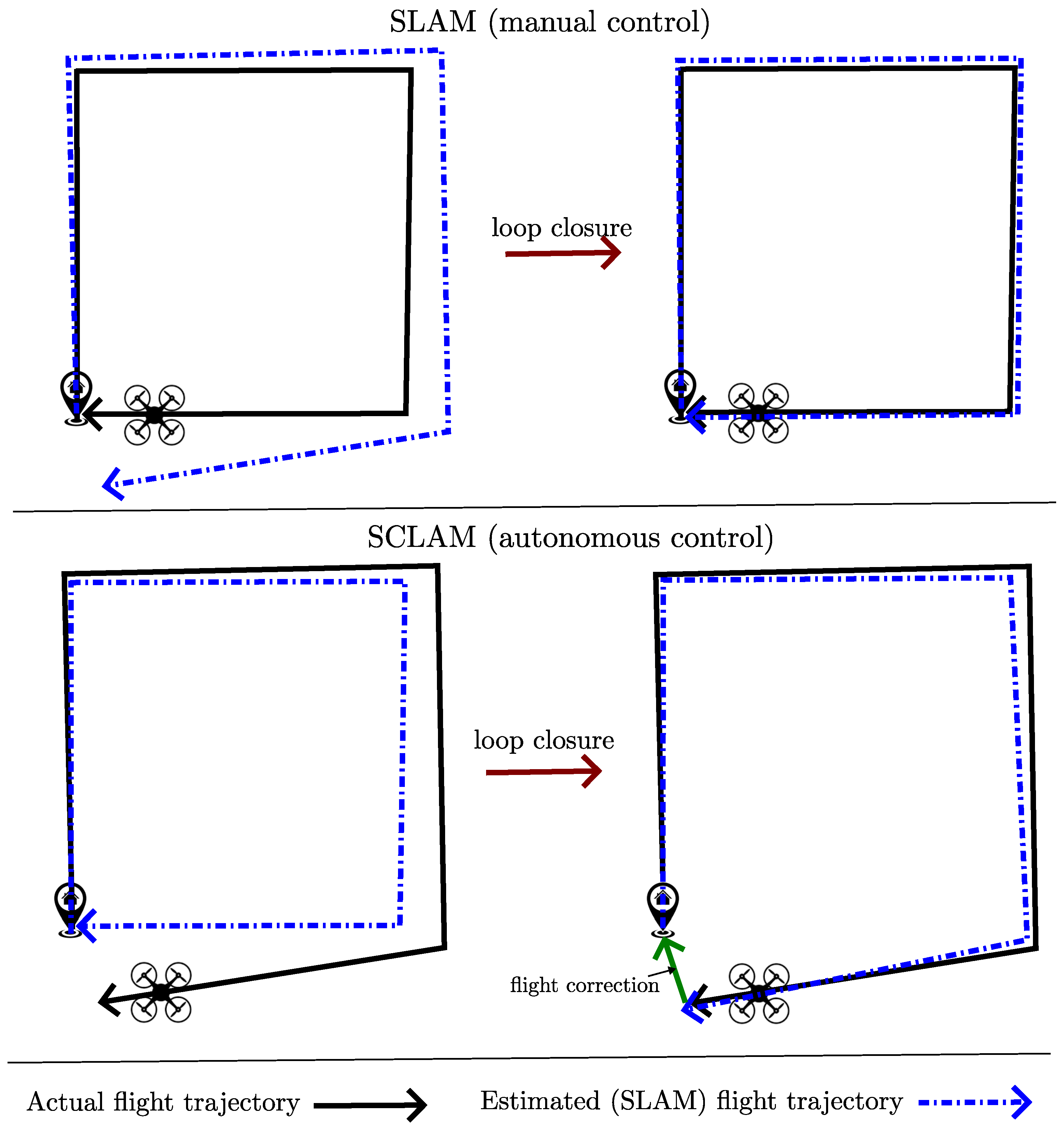
• When using SLAM methods (Figure 1, upper plots), it is common to assume perfect control, where the robot is manually guided along a predefined trajectory. As the robot moves farther from its starting position, the estimated trajectory will inevitably drift from the actual path due to integration errors. However, when the robot returns to its base and detects a previously mapped area (a process known as loop closure), the SLAM algorithm can reduce the accumulated error drift. The performance of the SLAM algorithm is then evaluated by comparing the estimated trajectory to the predefined path.
  

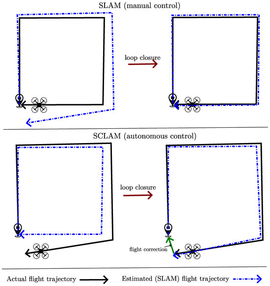  Figure 1. Comparison between the SLAM problem (upper plot) and the SCLAM problem (lower plot) regarding the actual and estimated trajectories before and after loop closure.
• Conversely, with SCLAM methods (Figure 1, lower plots), the pose estimated by the SLAM subsystem is directly fed back to the autonomous control subsystem. This means that the autonomous control treats the SLAM-estimated pose as the ground truth. Consequently, any error in the SLAM-estimated position will result in a corresponding error between the robot’s desired and actual positions. When a loop closure occurs, the estimated robot position is corrected, enabling the control subsystem to identify and adjust the actual drifted position of the robot.

4.2. System Architecture

Figure 2 depicts the architecture of the proposed SCLAM system. The flying robot is assumed to be a multi-rotor equipped with a monocular camera and a standard array of sensors commonly found in such devices, including an Inertial Measurement Unit (IMU), Altimeter (barometer), and others.

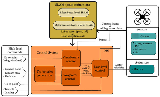
Figure 2. Proposed architecture.

The architecture comprises two key systems: SLAM and Control. The SLAM system processes the onboard robot’s sensor data stream to compute the robot’s state (pose and velocity). It also identifies and corrects trajectory loops to minimize error drift in estimates. Meanwhile, the Control system utilizes feedback from SLAM estimates and other sensor data to determine the rotor velocities necessary for the robot to execute high-level commands such as exploring an area or navigating to a specific point. In the following sections, each of these subsystems will be explained in detail.

4.3. SLAM System

The objective of the monocular-based SLAM system is to estimate the following robot state vector ${\mathbf{x}}_r$:

$${\mathbf{x}}_r={\left[\begin{array}{cccc}{\mathbf{e}}^{NR}& {\mathit{\omega }}^R& {\mathbf{r}}^N& {\mathbf{v}}^R\end{array}\right]}^T$$

(1)

The vector ${\mathbf{e}}^{NR}=\left[\theta ,\varphi ,\psi \right]$ describes the orientation of the robot’s coordinate frame ^R relative to the navigation coordinate frame ^N. Here, $\theta$, $\varphi$, and $\psi$ are the Tait–Bryan angles, also known as Euler angles, representing roll, pitch, and yaw, respectively. This work employs the intrinsic rotation sequence $\psi -\varphi -\theta$. The vector ${\mathit{\omega }}^R=[{\omega }_x,{\omega }_y,{\omega }_z]$ indicates the robot’s rotational velocity along the $x_R$, $y_R$, and $z_R$ axes defined in the robot frame ^R. The vector ${\mathbf{r}}^N=[x_r,y_r,z_r]$ represents the robot’s position as expressed in the navigation frame ^N. The vector ${\mathbf{v}}^R=[v_x,v_y,v_z]$ denotes the robot’s linear velocity along the $x_R$, $y_R$, and $z_R$ axes, as measured in the robot frame ^R.

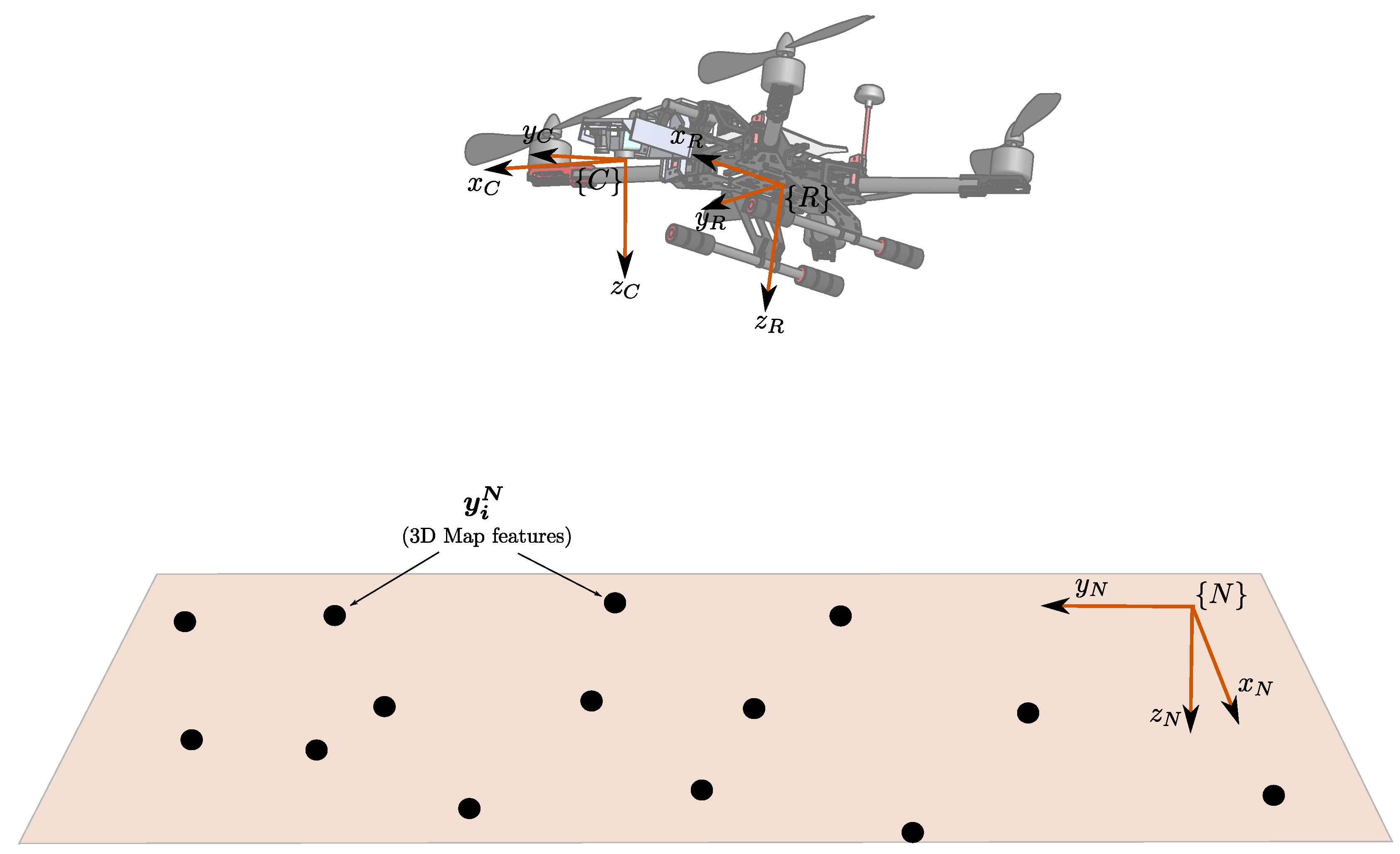
Since the proposed system is designed for local autonomous navigation tasks of robots, the local tangent frame serves as the navigation frame. This navigation frame, denoted as ^N, adheres to the NED (north-east-down) convention, with the robot’s initial position establishing its origin. In this study, all coordinate systems are right-handed. Quantities expressed in the navigation frame, the robot frame, and the camera frame are indicated by superscripts ^N, ^R, and ^C, respectively (refer to Figure 3).

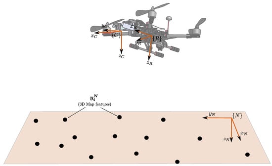
Figure 3. System parameterization.

The robot’s state vector ${\mathbf{x}}_r$ is estimated from a series of 2D visual measurements ${\mathbf{z}}_{uv}={[u_i,v_i]}^T$ corresponding to static 3D points ${\mathbf{y}}_i^N={[x_i,y_i,z_i]}^T$ in the robot’s environment. Additionally, a series of auxiliary measurements ${\mathbf{z}}_k$ are obtained from the robot’s onboard sensors, such as the following:

• Attitude measurements ${\mathbf{z}}_e={[\theta ,\varphi ,\psi ]}^T$, which are acquired from the Attitude and Heading Reference System (AHRS);
• Altitude measurements ${\mathbf{z}}_{z_r}=z_r$, which are obtained from the altimeter.

The SLAM system is designed to harness the strengths of two key methodologies in a visual-based SLAM system: filter-based methods and optimization-based methods. This integration leverages the complementary nature of these approaches. The system architecture includes a filter-based SLAM subsystem for continuous local SLAM processes and an optimization-based SLAM subsystem for maintaining a consistent global map of the environment. Running these components concurrently in separate processes enhances both modularity and robustness, providing an additional layer of redundancy.

A detailed description of the complete SLAM system can be found in a previous work by the author [24], with the source code also available at [25]. This work will focus on introducing the control functionality.

4.4. Control System

4.4.1. Low-Level Control

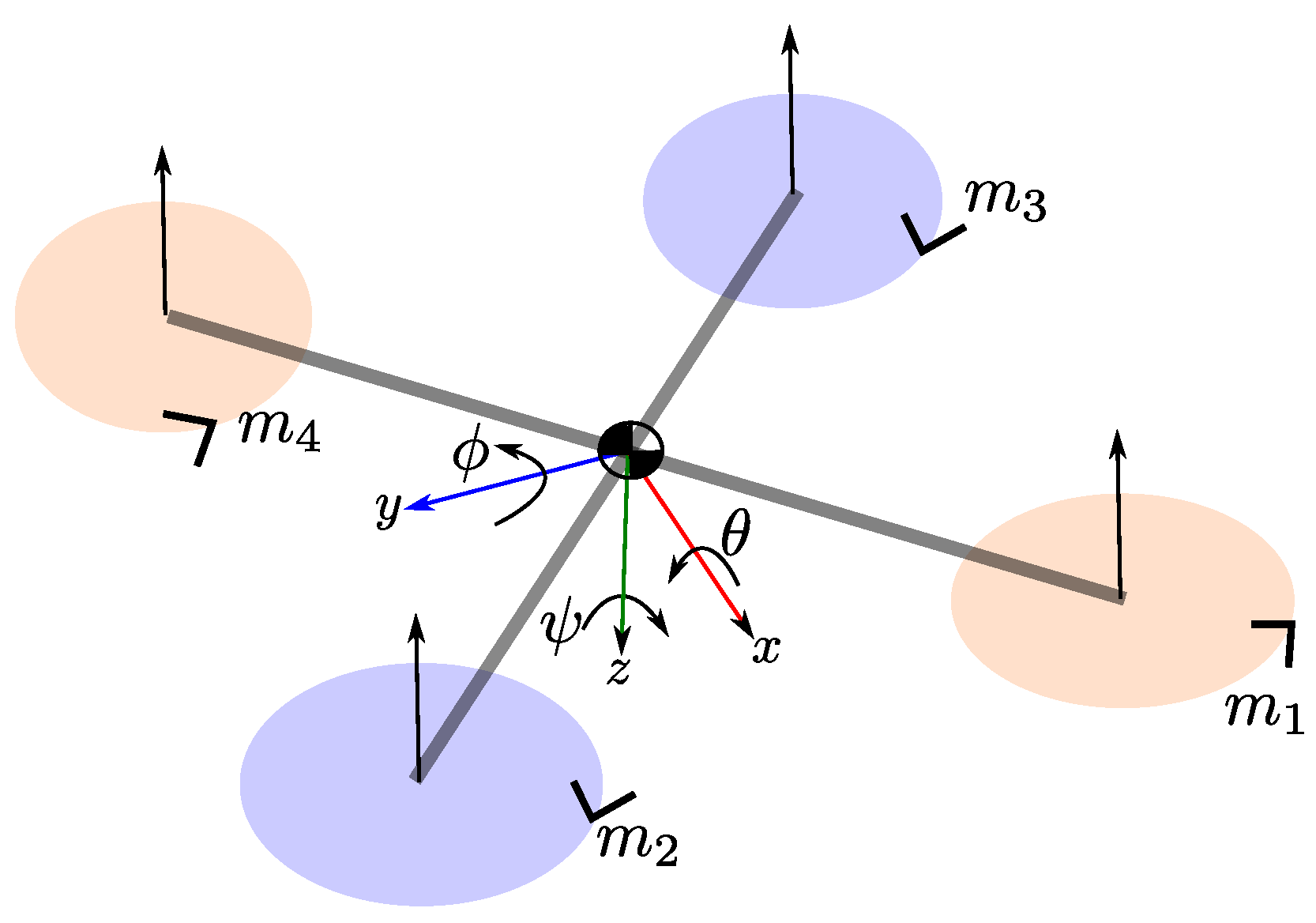
The goal of this subsystem is to manage the robot’s linear velocity along $(x-y)$ axes, as well as its altitude and yaw rate. Specifically, it calculates the required velocities for the robot’s rotors, denoted by $\mathbf{m}={[m_1,m_2,m_3,m_4]}^T$, which are necessary to achieve the desired control reference $\mathbf{r}=[v_x^{*R},v_y^{*R},v_z^{*N},{\omega }_z^{*R}]$. The components of the control reference are defined as follows: $v_x^{*R}$: the target linear velocity of the robot along the x-axis in the robot frame; $v_y^{*R}$: the target linear velocity of the robot along the y-axis in the robot frame; $v_z^{*N}$: the target linear velocity of the robot along the z-axis (altitude) in the navigation frame; ${\omega }_z^{*R}$: the target angular velocity of the robot along the z-axis (yaw) in the robot frame (see Figure 4).

Figure 4. Notation for the quad-rotor UAV used in this work, illustrating the rotors, thrust vectors, and directions of rotation.

To adjust its linear velocity along the x and y axes, the robot must vary its pitch and roll accordingly. To compute the reference signals for pitch ${\varphi }_{\mathrm{ref}}$ and roll ${\theta }_{\mathrm{ref}}$, which are necessary to achieve the desired velocities $v_x^{*R}$ and $v_y^{*R}$, Proportional–Integral (PI) controllers are employed:

$$\begin{array}{cc}\hfill & {\varphi }_{\mathrm{ref}}=K_{x,p}{e}_x+K_{x,i}\int e_x\hfill \\ \hfill & {\theta }_{\mathrm{ref}}=-(K_{y,p}{e}_y+K_{y,i}\int e_y)\hfill \end{array}$$

(2)

where $e_x=v_x^{*R}-v_x^R$ and $e_y=v_y^{*R}-v_y^R$ represent the error in velocities along the x and y axes, respectively. The parameters $K_{x,p}$ and $K_{x,i}$ are the proportional and integral gains for the x axis, while $K_{y,p}$ and $K_{y,i}$ are the proportional and integral gains for the y axis. The actual linear velocities $v_x^R$ and $v_y^R$ can be measured using the robot’s optical flow sensor. Alternatively, if the optical flow sensor is not available, $v_x^R$ and $v_y^R$ can be obtained from the SLAM output.

The low-level pitch ($u_{\varphi }$) and roll ($u_{\theta }$) inputs are computed using a Proportional–Derivative (PD) controller, while the low-level vertical ($u_z$) and yaw ($u_{\psi }$) inputs are computed using a Proportional (P) controller:

$$\begin{array}{cc}\hfill & u_{\theta }=K_{\theta ,p}\theta +{\omega }_x^R+{\theta }_{\mathrm{ref}}\hfill \\ \hfill & u_{\varphi }=K_{\varphi ,p}\varphi +{\omega }_y^R+{\varphi }_{\mathrm{ref}}\hfill \\ \hfill & u_z=K_{z,p}{e}_z\hfill \\ \hfill & u_{\psi }=K_{\psi ,p}{e}_{\psi }\hfill \end{array}$$

(3)

where $e_z=z_{\mathrm{ref}}-z_r^N$ and $e_{\psi }={\omega }_z^{*R}-{\omega }_z^R$ represent, respectively, the error in altitude and the error in angular velocity along the z axis. The vertical reference $z_{\mathrm{ref}}$ is updated according to the target linear velocity along the z axis: $z_{\mathrm{ref}}=z_{\mathrm{ref}}+v_z^{*N}\mathrm{\Delta }t$. The parameters $K_{\theta ,p}$, $K_{\varphi ,p}$, $K_{z,p}$, and $K_{\psi ,p}$ are the proportional gains, and $\mathrm{\Delta }t$ is the time step. The actual pitch ($\varphi$) and roll ($\theta$) can be obtained from the robot’s Attitude and Heading Reference System (AHRS). The actual angular velocities of ${\omega }_x^R$, ${\omega }_y^R$, and ${\omega }_z^R$ can be measured using the robot’s Inertial Measurement Unit (IMU). The actual altitude $z_r^N$ can be measured using the robot’s altimeter.

The robot’s rotors velocities ${[m_1,m_2,m_3,m_4]}^T$ are computed from the inputs vector ${[u_z,u_{\psi },u_{\varphi },u_{\theta }]}^T$ through the following linear system:

$$\left[\begin{array}{c}{m}_1\\ m_2\\ m_3\\ m_4\end{array}\right]=\left[\begin{array}{cccc}1& 1& 1& 1\\ 1& -1& 1& -1\\ 1& -1& -1& 1\\ 1& 1& -1& -1\end{array}\right]\left[\begin{array}{c}{u}_z\\ u_{\psi }\\ u_{\varphi }\\ u_{\theta }\end{array}\right]+\left[\begin{array}{c}{K}_{z,0}\\ K_{z,0}\\ K_{z,0}\\ K_{z,0}\end{array}\right]$$

(4)

where $K_{z,0}$ is a feed-forward constant representing the rotor velocity required to maintain the robot in a hovering position. The low-level controller presented in this section is the same as the one used by the DJI Mavic 2 Pro, the aerial robot employed in virtual experiments. However, it is important to note that other low-level control techniques can be used if needed.

The low-level control module directly manages two high-level commands:

• Take-off$<>$: To lift the robot from the ground when it is landed, the module sets the vertical reference $z_{\mathrm{ref}}$ to a value slightly greater than zero (e.g., 0.5 m).
• Landing$<>$: When the robot’s altitude is near the ground (e.g., less than 0.2 m), the command initiates landing by setting the rotor velocities to zero.

4.4.2. Waypoint Control

The goal of this subsystem is to manage the robot’s position and yaw. Specifically, it calculates the required velocities $[v_x^R,v_y^R,v_z^N,{\omega }_z]$ needed for the robot to move to the desired position (waypoint) $[x_r^{*N},y_r^{*N},z_r^{*N},{\psi }^{*}]$.

To achieve this, the following signal errors are computed:

$$\begin{array}{cc}\hfill & e_x^N=x_r^{*N}-x_r^N\hfill \\ \hfill & e_y^N=y_r^{*N}-y_r^N\hfill \\ \hfill & e_z^N=z_r^{*N}-z_r^N\hfill \\ \hfill & e_{\psi }={\psi }^{*}-\psi \hfill \end{array}$$

(5)

where $[x_r^N,y_r^N,z_r^N,\psi ]$ represents the actual position and yaw of the robot, which are obtained from the robot state vector ${\mathbf{x}}_r$ estimated by the SLAM system.

The x-y error is transformed from navigation coordinates to robot coordinates:

$$\left[\begin{array}{c}{e}_x^R\\ e_y^R\end{array}\right]=\left[\begin{array}{cc}cos\psi & sin\psi \\ -sin\psi & cos\psi \end{array}\right]\left[\begin{array}{c}{e}_x^N\\ e_y^N\end{array}\right]$$

(6)

A proportional control strategy with logarithmic smoothing is used to compute the velocities $[v_x^R,v_y^R,v_z^N,{\omega }_z]$:

$$\begin{array}{cc}\hfill & v_x^R=-k_{p_x}·{log}_{10}(\left|e_x^R\right|+1.0)·\mathrm{sign}\left(e_x^R\right)\hfill \\ \hfill & v_y^R=-k_{p_y}·{log}_{10}(\left|e_y^R\right|+1.0)·\mathrm{sign}\left(e_y^R\right)\hfill \\ \hfill & v_z^N=k_{p_z}·{log}_{10}(\left|e_z^N\right|+1.0)·\mathrm{sign}\left(e_z^N\right)\hfill \\ \hfill & {\omega }_z=k_{p_{\psi }}·{log}_{10}(\left|e_{\psi }\right|+1.0)·\mathrm{sign}\left(e_{\psi }\right)\hfill \end{array}$$

(7)

where parameters $k_{p_x}$, $k_{p_y}$, $k_{p_z}$, and $k_{p_{\psi }}$ are the proportional gains. At each time step, the computed velocities are sent as inputs to the low-level control module until the following condition is met:

$$(\left|e_x^N\right|<e_{xy,max})\mathrm{and}(\left|e_y^N\right|<e_{xy,max})\mathrm{and}(\left|e_z^N\right|<e_{z,max})\mathrm{and}(\left|e_{\psi }\right|<e_{\psi ,max})$$

(8)

where $e_{xy,max}$, $e_{z,max}$ and $e_{\psi ,max}$ are the maximum allowable errors for each position dimension. Thus, when the above condition is true, it is assumed that the robot has arrived at the desired waypoint. It is important to note that there is a trade-off when tuning the maximum allowable errors. Reducing these values will improve waypoint accuracy but this is also likely to increase the time required to reach each point due to the additional corrections needed to minimize the errors.

The waypoint control module directly manages the following high-level command:

• Go-to-point$<x_r^{*N},y_r^{*N},z_r^N,{\psi }^{*}>$: Commands the robot to move to the specified position and orientation.

4.4.3. Visual Marks-Based Control

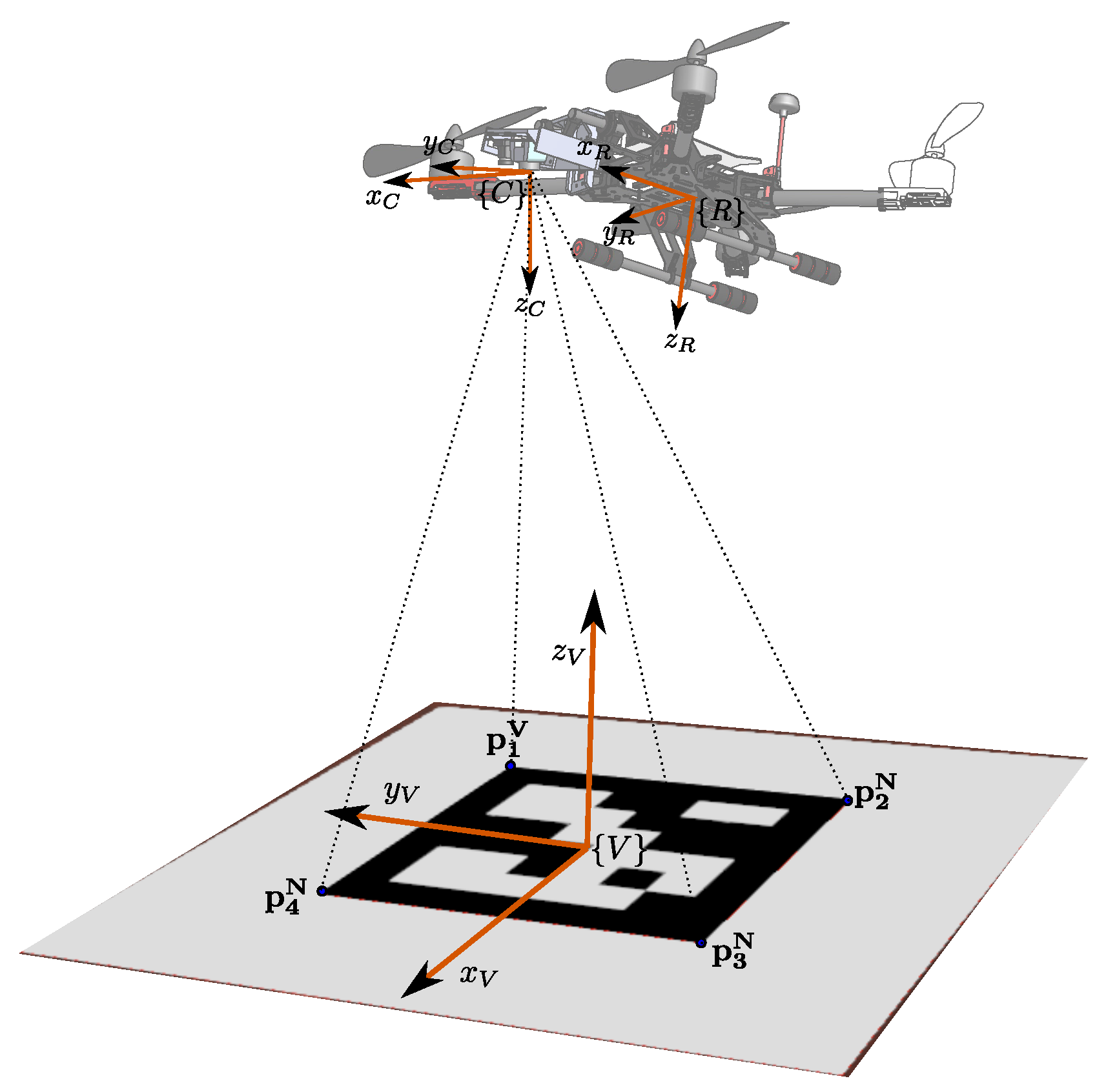
The goal of this subsystem is to manage the robot’s position and yaw relative to a visual reference. Specifically, it calculates the required velocities $[v_x^R,v_y^R,v_z^N,{\omega }_z]$ needed for the robot to move to the desired position $[x_r^{*V},y_r^{*V},z_r^{*V},{\psi }^{*V}]$, where the superscript ^V denotes a local coordinate frame attached to a visual marker (see Figure 5).

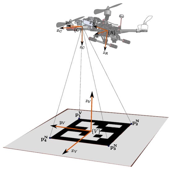
Figure 5. Reference frames used for visual marks-based control. An Aruco marker is used in this work.

To achieve this, the following signal errors are computed:

$$\begin{array}{cc}\hfill & e_x^N=x_r^{*V}-x_r^V\hfill \\ \hfill & e_y^N=y_r^{*V}-y_r^V\hfill \\ \hfill & e_z^N=z_r^{*V}-z_r^V\hfill \\ \hfill & e_{\psi }={\psi }^{*V}-{\psi }^V\hfill \end{array}$$

(9)

where $[x_r^V,y_r^V,z_r^V,{\psi }^V]$ represents the actual position and yaw of the robot with respect to the visual marker. These values are computed by solving the Perspective-n-Point (PnP) problem. The PnP problem involves determining the camera pose based on a set of known 3D points (i.e., anchors) in the scene and their corresponding 2D projections in the image captured by the camera [26].

In this case, let ${\mathbf{h}}_i({\mathbf{c}}_H^V,{\mathbf{p}}_i^V)$ denote the predicted projection of the 3D point ${\mathbf{p}}_i^V$ in the image plane, and ${\mathbf{v}}_i$ denote the measured (matched) projection of ${\mathbf{p}}_i^V$ in the image plane. Also, let ${\mathbf{c}}^V$ represent the camera pose defined in the visual marker frame. The PnP problem can be formulated as the minimization of the total reprojection error $d({\mathbf{h}}_i({\mathbf{c}}^V,{\mathbf{p}}_i^V),{\mathbf{v}}_i)$ for n points ${\mathbf{p}}_i^V$. This can be expressed mathematically as follows:

$$\underset{{\mathbf{c}}^V}{min}\sum _{i=1}^{n}d{({\mathbf{h}}_i({\mathbf{c}}^V,{\mathbf{p}}_i^V),{\mathbf{v}}_i)}^2$$

(10)

Here, ${\mathbf{c}}^V$ represents the estimated camera pose with respect to the visual marker frame that minimizes the PnP problem. In this work, the aruco::estimatePoseSingleMarkers method from the OpenCV library [27] is used to solve this (10).

Velocities $[v_x^R,v_y^R,v_z^N,{\omega }_z]$ are computed using the same proportional control strategy with logarithmic smoothing described in Equations (6)–(8).

The visual-mark control module directly manages the following high-level command:

• Go-to-point-visual$<x_r^{*V},y_r^{*V},z_r^V,{\psi }^{*V}>$: Commands the robot to move to the specified position and orientation respect to the visual mark.

4.4.4. Trajectory Generation

The goal of this subsystem is to generate flight trajectories that address high-level commands, such as ’Explore Area’ or ’Go Home,’ by computing the waypoints that compose these trajectories.

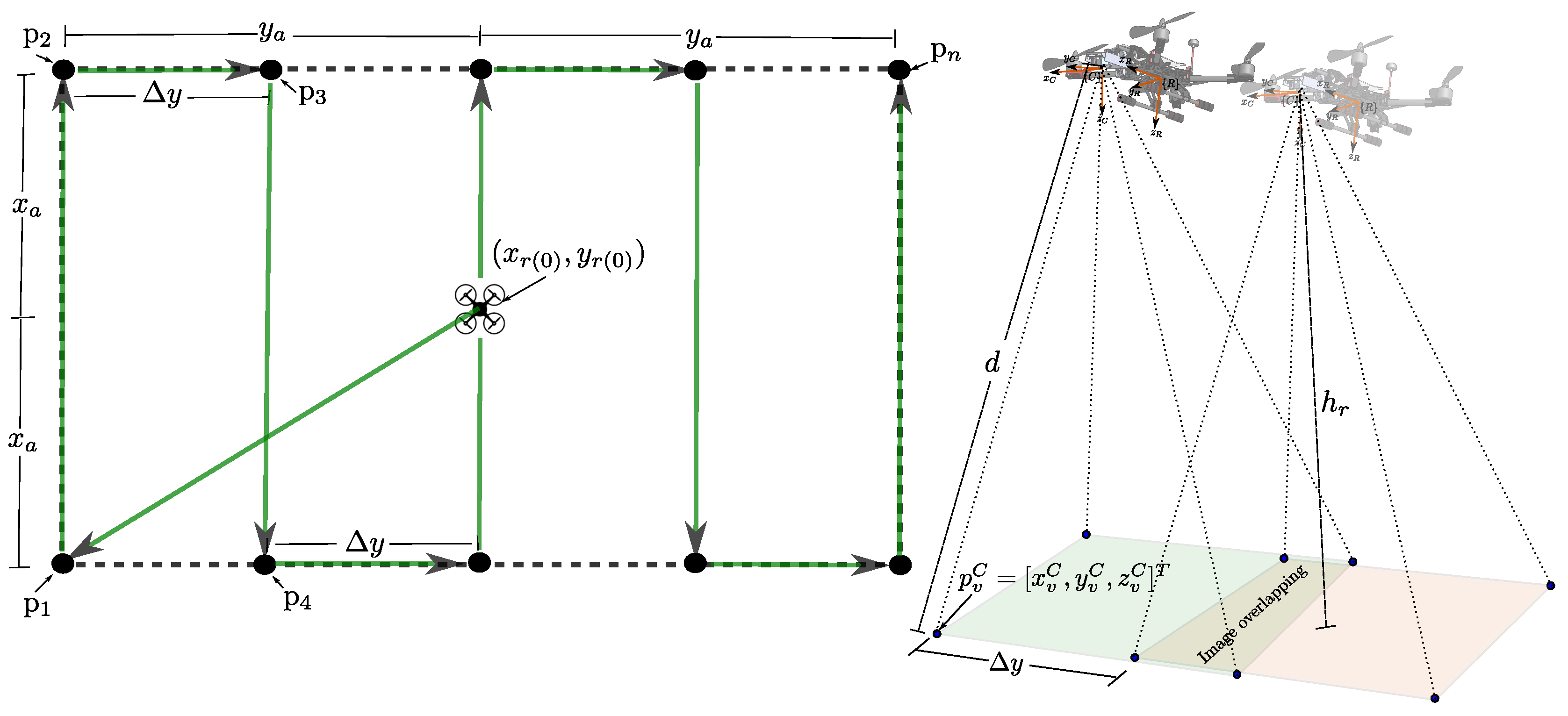
Explore-area$<x_a,y_a,{\lambda }_y>$ generates a series of n waypoints p₁, p₂,...,p_n that compose a flight trajectory, as illustrated in Figure 6. This trajectory is designed to explore a rectangular area of $2\ast x_a\times 2\ast y_a$ with a constant altitude $z_r^N$ and yaw ψ for a robot initially positioned at $[x_{r\left(0\right)}^N,y_{r\left(0\right)}^N,z_{r\left(0\right)}^N,{\psi }_{\left(0\right)}]$. In this case, p_i is defined as the i-th waypoint, p_i$=[x_{r\left(i\right)}^N,y_{r\left(i\right)}^N,z_{r\left(0\right)}^N,{\psi }_{\left(0\right)}]$, that composes the trajectory.

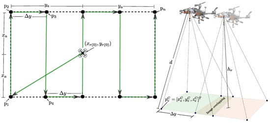
Figure 6. Pattern used by the Explore-area command (left plot) and side image overlap illustration (right plot).

In the flight pattern illustrated in Figure 6 (left plot), $\mathrm{\Delta }y=f({\lambda }_y,h_r)$ represents the displacement between each segment of the flight trajectory along the y-axis. This displacement determines the degree of image overlap, as shown in the right plot. Specifically, $\mathrm{\Delta }y$ depends on the local altitude of the robot $h_r$ and the overlapping factor ${\lambda }_y$. In aerial photogrammetry, image overlapping refers to the intentional overlap of consecutive aerial images captured during a flight. Effective overlapping is essential for generating high-quality orthoimages, digital elevation models (DEMs), and other products, as it allows for reliable stitching of images and improved data integrity.

First, the displacement $\mathrm{\Delta }y$ that satisfies the overlapping factor ${\lambda }_y$, given the robot’s current altitude $h_r$, is computed. To achieve this, we calculate the position of a virtual landmark ${\mathbf{p}}_v^C={[x_v^C,y_v^C,z_v^C]}^T$ with respect to the camera frame from the following equation:

$${\mathbf{p}}_v^C=d\ast {\mathbf{h}}_c$$

(11)

where $d=h_v/{\mathbf{h}}_c·{[0,0,1]}^T$ is the depth of the virtual feature ${\mathbf{p}}_v^C$ and ${\mathbf{h}}_c=f{(u,v)}^{-1}$ is the normalized vector pointing from the optical center of the camera to the virtual feature ${\mathbf{p}}_v^C$. Here, $f{(u,v)}^{-1}$ denotes the inverse of the camera projection model (see [24]), and u and v are the column and row dimension corresponding to the image resolution, respectively. The robot’s current altitude $h_r$ can be obtained directly from a range sensor or computed using the local SLAM map.

Given the above, $\mathrm{\Delta }y$ is computed as follows:

$$\mathrm{\Delta }y=\left|y_v^C\right|(1+{\lambda }_y)$$

(12)

where ${\lambda }_y\in (-1,\infty )$. Note that $\mathrm{\Delta }y$ can range from just above zero to infinity.

The first waypoint p₁, corresponding to the left-lower corner of the trajectory, is computed as follows:

$${\mathbf{p}}_1=[(x_{r\left(i\right)}^N+x_a),(y_{r\left(i\right)}^N-y_a),z_{r\left(0\right)}^N,{\psi }_{\left(0\right)}].$$

The remaining $n-1=(4\ast \lfloor y_a\rfloor /\mathrm{\Delta }y)+1$ waypoints p₂,...,p_n are computed using Algorithm 1.

Algorithm 1 Waypoints p2,...,pn generation

1: $right\leftarrow false$ 2: $c\_lr\leftarrow 0$ 3: for $i\leftarrow 2$ to $(4\ast \lfloor y_a\rfloor /\mathrm{\Delta }y+3)$ do 4:     $c\_lr\leftarrow c\_lr+1$ 5:     if $right$ then 6:         $x_{r\left(i\right)}^N\leftarrow x_{r\left(0\right)}^N+x_a$ 7:         $y_{r\left(i\right)}^N\leftarrow y_{r\left(0\right)}^N-y_a$ 8:         if $c\_lr=2$ then 9:            $right\leftarrow false$ 10:            $c\_lr\leftarrow 0$ 11:         else 12:            $y_a\leftarrow y_a-\mathrm{\Delta }y$ 13:         end if 14:     else 15:         $x_{r\left(i\right)}^N\leftarrow x_{r\left(0\right)}^N-x_a$ 16:         $y_{r\left(i\right)}^N\leftarrow y_{r\left(0\right)}^N-y_a$ 17:         if $c\_lr=2$ then 18:            $right\leftarrow true$ 19:            $c\_lr\leftarrow 0$ 20:         else 21:            $y_a\leftarrow y_a-\mathrm{\Delta }y$ 22:         end if 23:         $z_{r\left(i\right)}^N\leftarrow z_{r\left(0\right)}^N$ 24:         ${\psi }_{\left(i\right)}\leftarrow {\psi }_{\left(0\right)}$ 25:     end if 26: end for

Finally, using the command Go-to-point$<x_r^{*N},y_r^N,z_r^N,\psi >$, each waypoint p_i with $i=1,\dots ,n$, which was computed previously, is executed sequentially to guide the robot in exploring the desired area. If a closing-loop condition occurs, the method terminates and returns a true value.

Go-home$<>$ moves the robot from its current position $[x_r^N,y_r^N,z_r^N,\psi ]$ to the home (hovering) position $[0^N,0^N,z_r^N,0]$. At first glance, one might think that this could be achieved simply by using Go-to-point$<0,0,z_r^N,0>$. However, the accumulated error drift in the estimated trajectory (see Section 4.1) can cause the robot to be far from the home position, even when it “thinks” it has returned.

One way to determine if the robot has successfully returned near the home position is to visually recognize the home. In this work, an Aruco marker (see Figure 5) located at the ground level of the home position is used to facilitate this task. Moreover, if the home position is recognized, the SLAM algorithm can close the loop and minimize the accumulated error drift in the estimated trajectory. If the robot is commanded to return to its home but the home is not visually recognized (and the loop is not closed) during the flight trajectory, it is assumed that the robot has lost track of the home position due to accumulated error drift in the SLAM estimates.

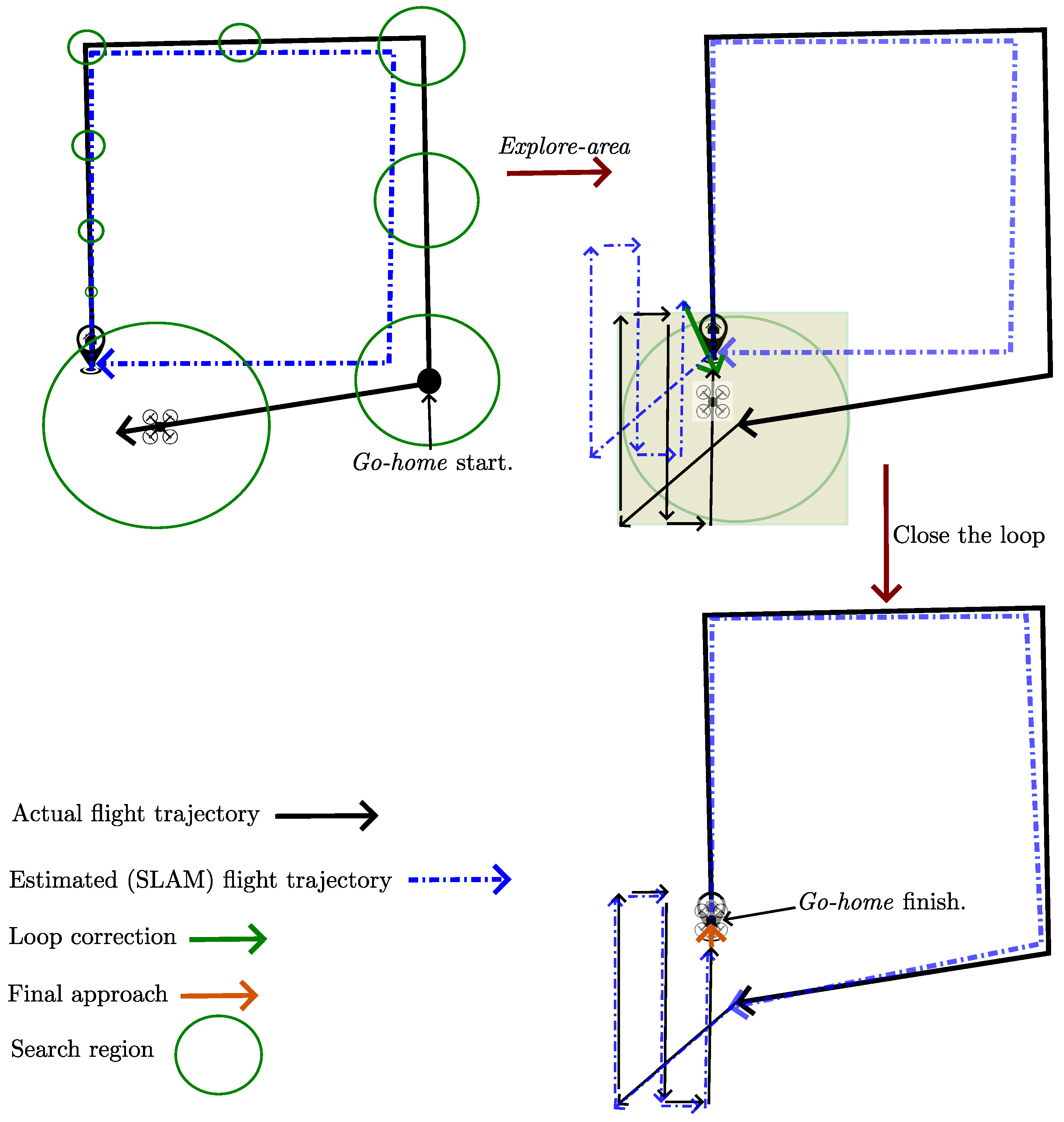
The approach to tackle the above problem is to define a search region, the size of which is determined by the following simple uncertainty model:

$$\dot{r}\left(t\right)=\xi \left(t\right)$$

(13)

where r is the radius of the search area, and $\xi \left(t\right)$ represents zero-mean Gaussian white noise with power spectral density defined by ${\sigma }_r^2$, specifically $\xi \left(t\right)\sim \mathcal{N}(0,{\sigma }_r^2)$. In this case, ${\sigma }_r$ is heuristically set to conservatively account for the increasing error drift in the estimated trajectory. This is performed in such a way that, when the robot “thinks” it has returned to the home position, the true home position lies within the search area (see Figure 7, upper-left plot).

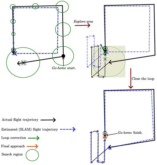
Figure 7. The go-home command utilizes an uncertainty model to define a search region for locating the visual marker at the home position when it is not found in the expected location due to accumulated error drift (upper-left plot). The explore-area method, constrained to this search region, is then used to locate the home position (upper-right plot). If the home is detected, the SLAM system closes the loop, minimizing pose error and allowing the robot to successfully navigate to the home position (lower-right plot).

Then, the robot is commanded to explore the search region using the command Explore-area$<r,r,{\lambda }_y>$ to try to find the home (see Figure 7, upper-right plot). If the home is recognized and the SLAM system closes the loop during the exploration, then the corrected position of the robot is obtained, and a final (small) approach to $[0^N,0^N,z_r^N,0]$ is commanded (see Figure 7, lower-right plot).

Algorithm 2 summarizes the Go-home $<>$ command.

Algorithm 2 Go-home$<>$ command

1: $Success\leftarrow \mathit{Go}-\mathit{to}-\mathit{point}<0,0,z_r^N,0>$ 2: if  $Success$  then 3:     if $CloseLoop$ then 4:         $Success\leftarrow \mathit{Go}-\mathit{to}-\mathit{point}<0,0,z_r^N,0>$ 5:         if $Success$ then 6:            Go-home successful!! 7:            Return true 8:         end if 9:     else 10:         $Success\leftarrow \mathit{Explore}-\mathit{area}<r,r,{\lambda }_y>$ 11:         if $CloseLoop$ then 12:            $Success\leftarrow \mathit{Go}-\mathit{to}-\mathit{point}<0,0,z_r^N,0>$ 13:            if $Success$ then 14:                Go-home successful!! 15:                Return true 16:            end if 17:         else 18:            Go-home unsuccessful!! 19:            Return false 20:         end if 21:     end if 22: end if

5. Results

The proposed visual-based SCLAM system was implemented in C++ within the ROS 2 (Robot Operating System 2) framework [28]. Each subsystem described in the system architecture (see Figure 2) has been developed as a ROS 2 component. Additionally, Webots was utilized for testing the system. Webots is widely recognized in research, education, and industry for prototyping and testing robotic algorithms in a virtual environment prior to real-world deployment [29]. The source code for implementing the proposed visual-based SCLAM system is available at [30].

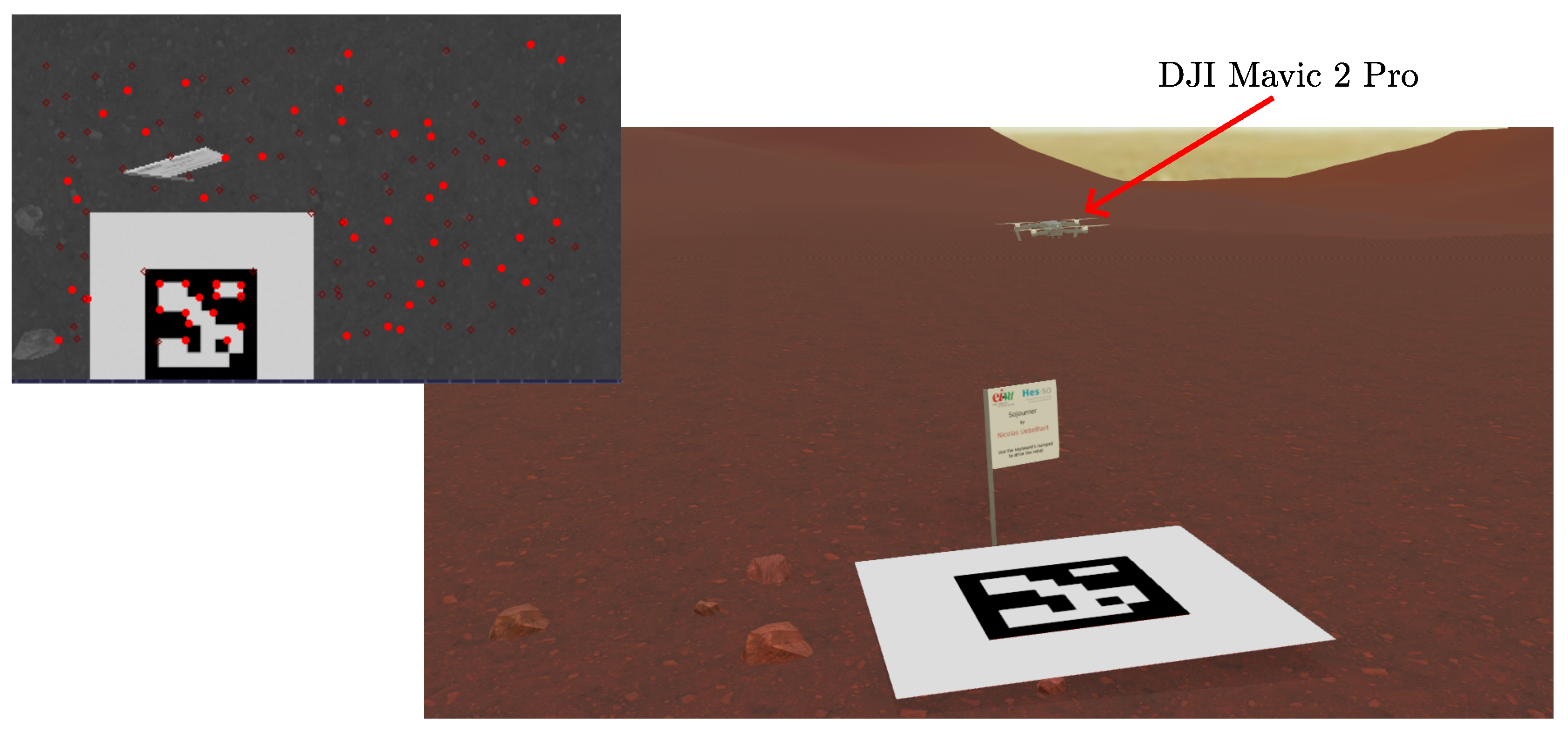
Figure 8 illustrates the Mars-like environment used in the virtual experiments, along with a frame captured by the downward-facing monocular camera of the robot, showcasing the visual features tracked at that moment. The flying robot used in our virtual experiments is a DJI Mavic 2 Pro. For our analysis, we capture image frames from the front monocular camera at a resolution of 400 × 240 pixels and a rate of 30 frames per second. Additionally, we also incorporate measurements from the IMU and altimeter.

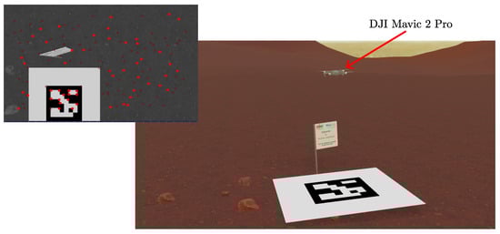
Figure 8. Virtual experiments were conducted in a Mars-like environment using the Webots simulator (main plot). A frame captured from the robot’s onboard camera shows the visual landmarks tracked by the SLAM system (upper-left plot).

5.1. Low-Level Control

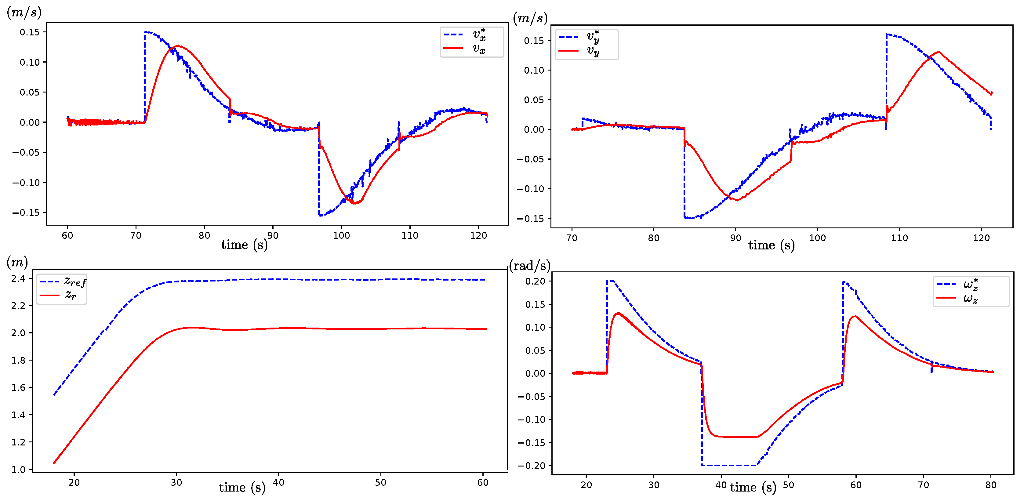
Figure 9 compares each low-level control signal reference $v_x^{*R}$, $v_y^{*R}$, $z_{\mathrm{ref}}$, and ${\omega }_z^{*R}$ with their corresponding actual responses $v_x^R$, $v_y^R$, $z_r^N$, and ${\omega }_z^R$. The reference altitude is defined as $z_{\mathrm{ref}}=z_{\mathrm{ref}}+v_z^{*N}\mathrm{\Delta }t$.

Figure 9. Comparison between reference signals $v_x^{*R}$, $v_y^{*R}$, $z_{\mathrm{ref}}$, and ${\omega }_z^{*R}$ and their responses $v_x^R$, $v_y^R$, $z_r^N$, and ${\omega }_z^R$ obtained from the low-level control subsystem.

It is observed that the low-level control system effectively tracks the reference inputs. For the linear velocities $v_x^{*R}$ and $v_y^{*R}$, the integral terms minimize steady-state error. In contrast, the altitude and yaw velocity control employ a Proportional (P) controller, leading to inherent steady-state errors in their outputs. These steady-state errors in altitude and yaw are subsequently managed by the high-level control system.

5.2. Waypoint Control

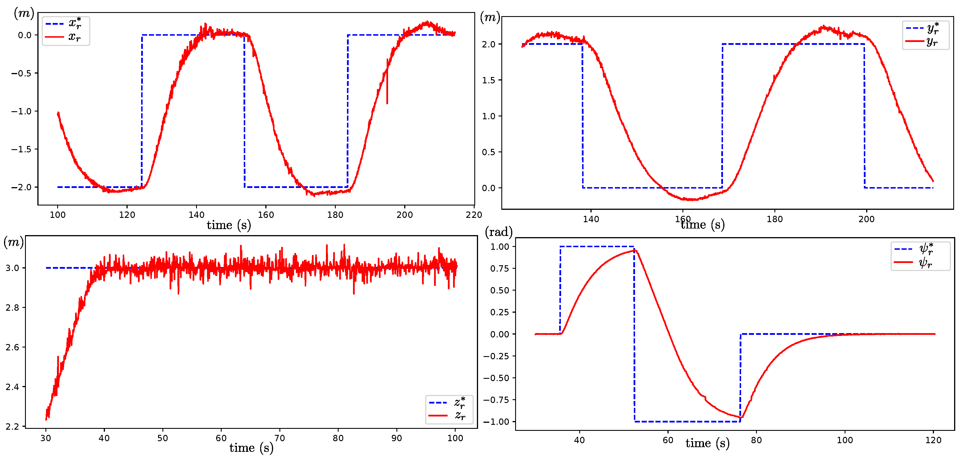
Figure 10 compares each waypoint control signal reference $x_r^{*N}$, $y_r^{*N}$, $z_r^{*N}$, and ${\psi }_r^{*}$ with their corresponding actual responses $x_r^N$, $y_r^N$, $z_r^N$, and ${\psi }_r$.

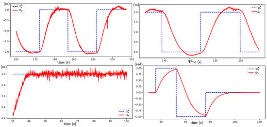
Figure 10. Comparison between reference signals $x_r^{*N}$, $y_r^{*N}$, $z_r^{*N}$, and ${\psi }_r^{*}$ and their responses $x_r^N$, $y_r^N$, $z_r^N$, and ${\psi }_r$ obtained from the waypoint control subsystem.

It is observed that the waypoint control system effectively tracks the reference inputs, indicating that the flying robot can move to the desired position and orientation within its environment. Furthermore, the control strategy incorporating logarithmic smoothing allows for the handling of arbitrarily large initial errors in pose.

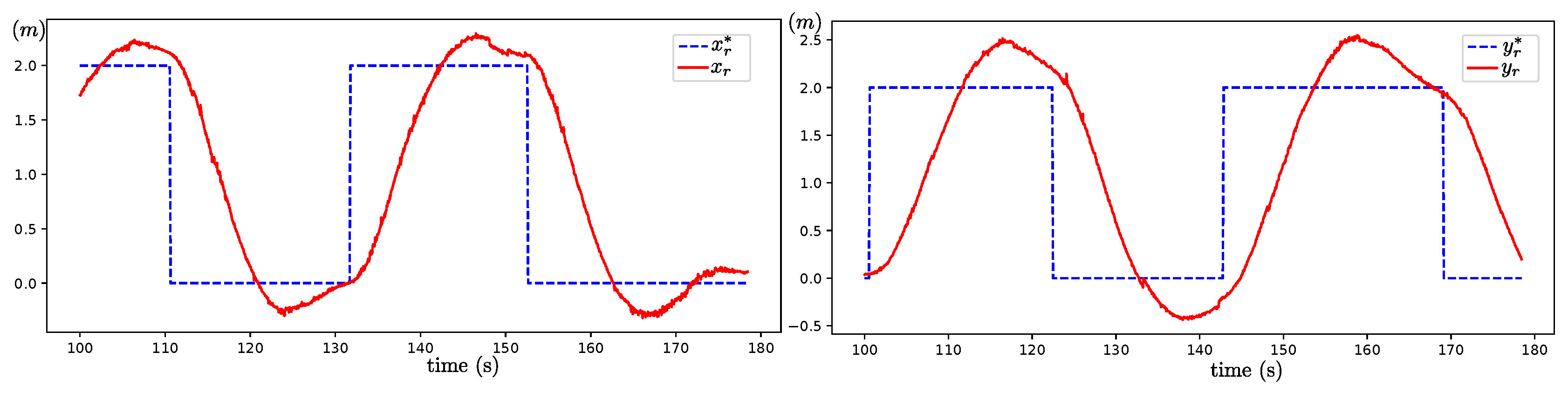
The results presented in Figure 10 were obtained by conservatively tuning the controller ($k_{p_x}=k_{p_y}=e_{xy,\max }=0.5$). Figure 11 shows the results for the reference signals $x_r^{*N}$ and $y_r^{*N}$, but in this case with slightly increased parameter values ($k_{p_x}=k_{p_y}=e_{xy,\max }=0.75$). These results demonstrate a faster response but at the cost of a larger overshoot. Alternatively, the low-level controller could be tuned alongside the waypoint controller to achieve different responses if needed. However, other control strategies could also be employed, particularly if more aggressive responses are required.

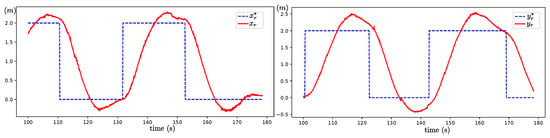
Figure 11. Comparison between the reference signals $x_r^{*N}$ and $y_r^{*N}$, and their corresponding responses $x_r^N$ and $y_r^N$, obtained by slightly increasing the control gains $k_{p_x}$ and $k_{p_y}$, as well as the maximum allowable error $e_{xy,\max }$.

5.3. Visual-Mark-Based Control

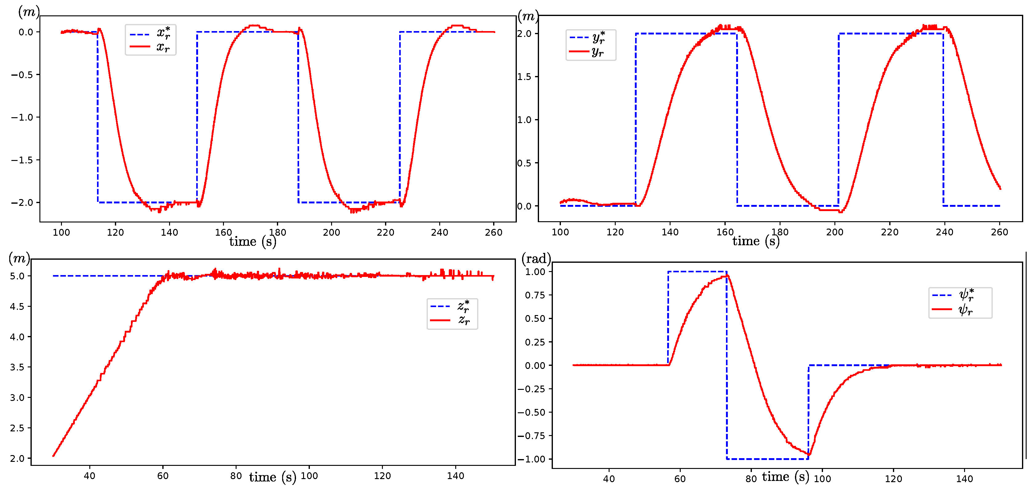
Figure 12 compares each signal reference $x_r^{*V}$, $y_r^{*V}$, $z_r^{*V}$, and ${\psi }_r^{*V}$ provided to the visual-mark-based control system with their corresponding actual responses $x_r^V$, $y_r^V$, $z_r^V$, and ${\psi }_r^V$.

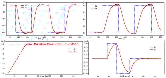
Figure 12. Comparison between reference signals $x_r^{*V}$, $y_r^{*V}$, $z_r^{*V}$, and ${\psi }_r^{*V}$ and their responses $x_r^V$, $y_r^V$, $z_r^V$, and ${\psi }_r^V$ obtained from the Visual-mark-based control subsystem.

It is observed that the visual-mark-based control system effectively tracks the reference inputs, indicating that the flying robot can move to the desired position and orientation relative to the Aruco visual mark. This controller requires the visual mark to be within the field of view of the robot’s onboard camera. Consequently, its working space is constrained to the area above the visual mark, with its size dependent on the robot’s altitude above the mark. In this case, the robot was commanded to fly at an altitude of 5 m to perform the desired trajectory over the x-y plane.

5.4. Explore Area

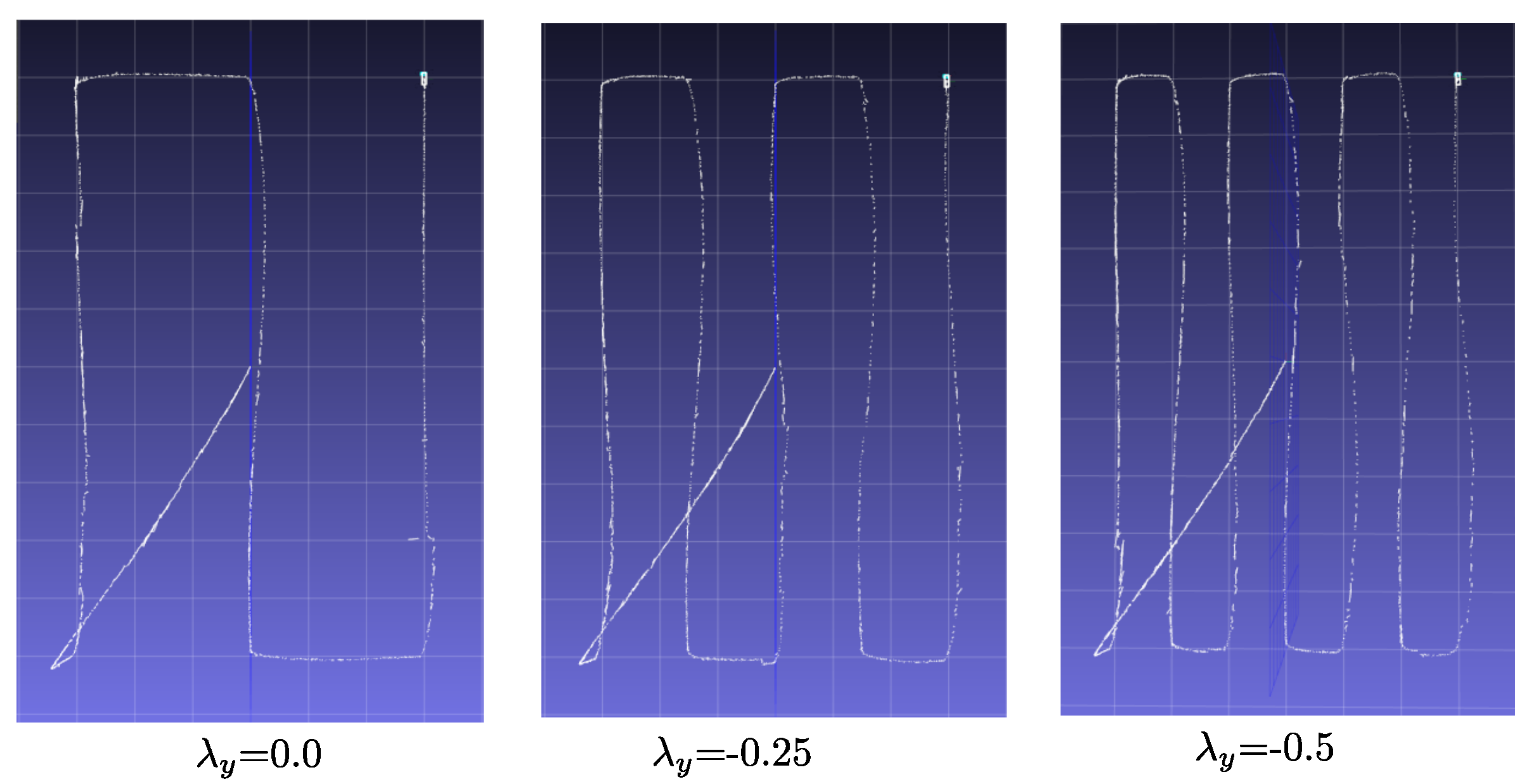
Figure 13 presents a comparison of the robot’s flying trajectories obtained using the command Explore-area $<5,3,{\lambda }_y>$ at an altitude of 3. The parameter values for ${\lambda }_y$ are set to $\{0.0,-0.25,-0.5\}$. With this command, the robot explores a rectangular area measuring 5 × 3 m, as detailed in Section 4.4.4.

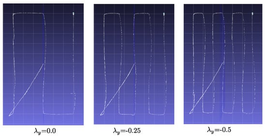
Figure 13. Comparison of trajectories obtained from the Explore-area command using three different values for ${\lambda }_y$.

The overlapping factor ${\lambda }_y$ determines the degree of image side overlap, which refers to the overlap between images captured from adjacent flight lines. As observed in the figure, the amount of overlap increases from the left plot to the right plot.

5.5. Full Exploration Mission

In this experiment, the following autonomous exploration mission was assigned to the robot:

• Take-off$<>$→Go-to-point-visual$<0,0,3,0>$→Go-to-point$<-25,0,3,0>$
  →Explore-area$<5,15,0>$→Go-to-point$<-15,15,3,0>$→Go-to-point$<-15,0,3,0>$→Go-home$<>$→Landing$<>$

The objective is to evaluate the entire SCLAM system by commanding the flying robot to autonomously take-off, navigate to a point distant from its home, explore an area of the environment, and then return to its home position to land. In scenarios where GPS is available, executing this mission would be relatively straightforward, potentially requiring only a visual-servoing control scheme to refine the landing process. Conversely, in GPS-denied environments, the accumulated error in the estimated pose throughout the trajectory leads to a discrepancy between the robot’s desired and actual positions, as discussed in Section 4.1. This issue is addressed by the ”Go-home” strategy outlined in Section 4.4.4.

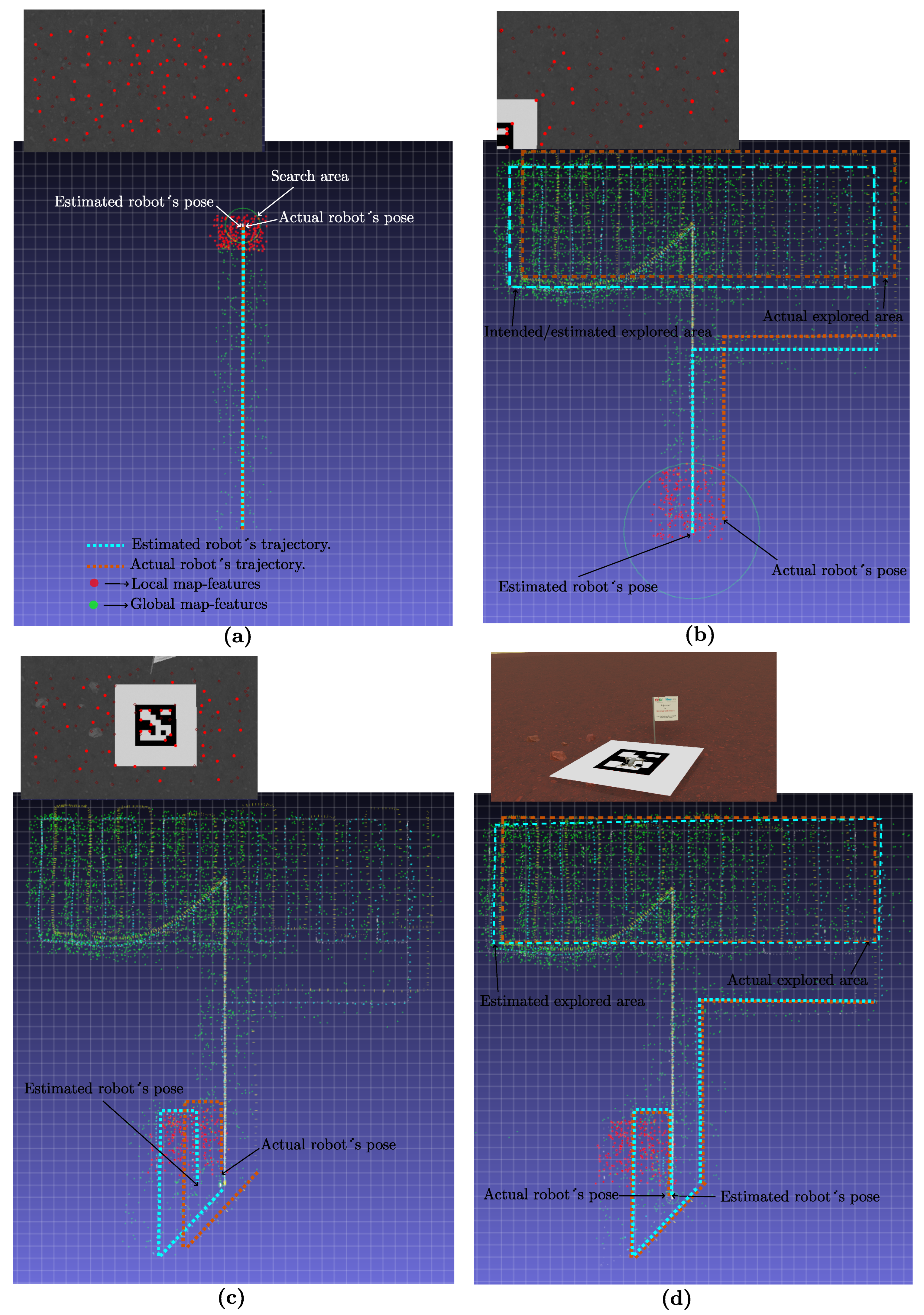
Figure 14 presents the results obtained from the previously described mission. Plot (a) shows the moment when the robot has just completed the command Go-to-point$<-25,0,3,0>$ and is about to execute the command Explore-area$<5,15,0>$. At this point, there is minimal error drift, but the search area defined by the uncertainty model (13) has begun to expand. In Plot (b), the robot has finished exploring and is in the process of executing the command Go-home$<>$, having returned to the position where it is supposed to recognize its home. However, due to the accumulated error in the estimated pose, the home position is not recognized, prompting the robot to search for it within the region defined by the search area. The accumulated error drift in the estimated robot’s pose also affects the accuracy of the Explore-area$<>$ command. In this case, Plot (b) also shows a comparison between the desired area to be explored using the Explore-area$<5,15,0>$ command and the actual area explored.

Figure 14. Plots (a–d) show the map, estimated, and actual robot trajectories obtained from a fully autonomous exploration mission at four different stages. Camera frames captured at each stage are displayed in plots (a–c). Note that the robot successfully returned to and landed at the home position (plot (d)) after correcting for accumulated error drift.

In Plot (c), the robot is traversing the home area while exploring the search area. At this stage, the SLAM system successfully detects the visual marker, enabling loop closure. In Plot (d), the SLAM system has closed the loop, effectively minimizing error drift, which means that the estimated pose of the robot aligns with its actual pose. Consequently, the robot is now able to execute the final approach to the home position and land. Additionally, after loop closure, it can be observed how the estimated global map, computed during the flight trajectory produced by the Explore-area$<>$ command (indicated in Plot (d) as the Estimated explored area), more closely corresponds to the actual explored area.

The accuracy of the Go-home process was evaluated by calculating the Mean Absolute Error (MAE) of the distance between the UAV’s home position and landing position across 20 experimental runs. The result was $0.12\pm 0.06\sigma$ m.

Table 1 and Table 2 provide statistics regarding the Local and Global SLAM processes, respectively. It can be observed that the duration of the autonomous flying mission was approximately 14 min (837 s), during which a global map comprising 56,412 landmarks was constructed. Additionally, it is noteworthy that the computation times for both the local and global SLAM processes are shorter than the execution time, indicating real-time performance.

Table 1. Statistics of the local SLAM process. In this table, feats:I/D is the relation between the total number of initialized and the deleted EKF features, Feat/Frame is the average number of features per frame, Time(s)/Frame is the average computation time per frame, and Comp/Exec Time(s) is the relation between the total computation time and total execution time.

	Feats:I/D	Feat/Frame	Time(s)/Frame	Comp/Exec Time(s)
Local SLAM	36,610/36,421	194.5 ± 11.80$\sigma$	0.0261 ± 0.010$\sigma$	526.05/836.90

Table 2. Statistics of the global mapping process. In this table, number KF is the total number of Key-frames contained by the global map, Anchors:I/D is the relation between the number of initialized and deleted anchors carried out by the global mapping process, Time(s)/Frame is the average computation time per update, and Comp/Exec Time(s) is the relation between the total computation time and total execution time.

	Number KF	Anchors:I/D	Time per Update (s)	Comp/Exec Time(s)
Global Map	555	88,350/31,938	0.354602 ± 0.12	197.15/836.90

5.6. Experiment in an Indoor Environment

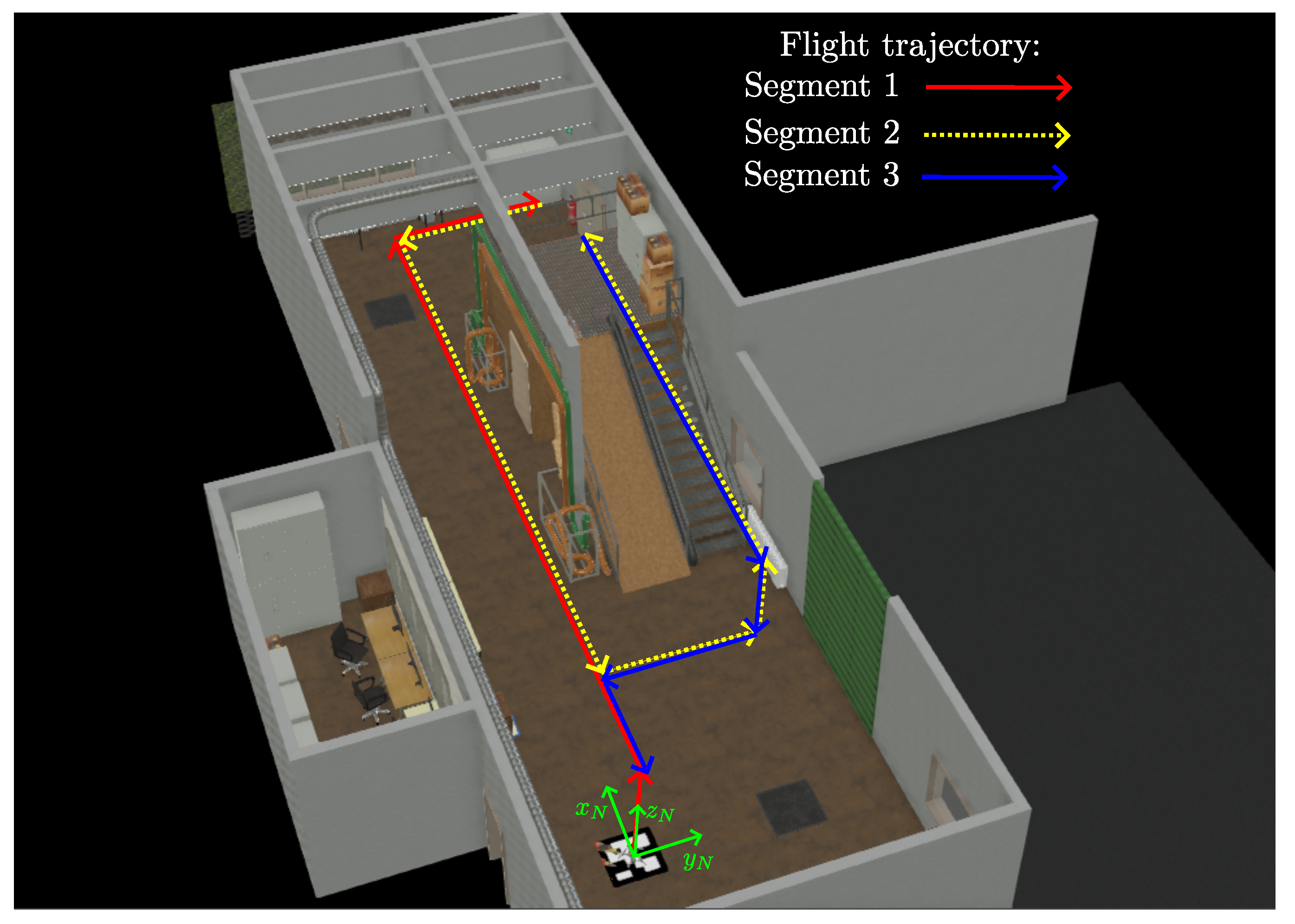
To gain deeper insights into the performance of the proposed visual-based SCLAM system, additional virtual experiments were conducted in a factory-like indoor environment. Figure 15 illustrates the environment and the flight trajectory employed in these experiments. To enhance the clarity of the experimental results, the trajectory is divided into three segments, each represented by a distinct color. The same flying robot, with the same sensor configuration used in previous experiments, was employed here.

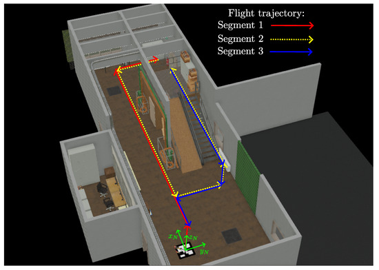
Figure 15. Virtual experiments were conducted in a controlled, factory-like indoor environment. The flight trajectory is represented in three distinct color segments for easier interpretation.

In this experiment, the following autonomous exploration mission was assigned to the robot: Take-off$<>$ → Go-to-point-visual$<0,0,3,0>$ → Go-to-point$<15,0,3,0>$ → Go-to-point$<15,3,3,0>$ → Go-to-point$<15,0,3,0>$ → Go-to-point$<3,0,3,0>$ → Go-to-point$<3,3,3,0>$ → Go-to-point$<3,3,4,0>$ → Go-to-point$<10,3,4,0>$ → Go-to-point$<3,3,4,0>$ → Go-to-point$<3,3,3,0>$ → Go-to-point$<3,0,3,0>$ → Go-home$<>$ → Landing$<>$

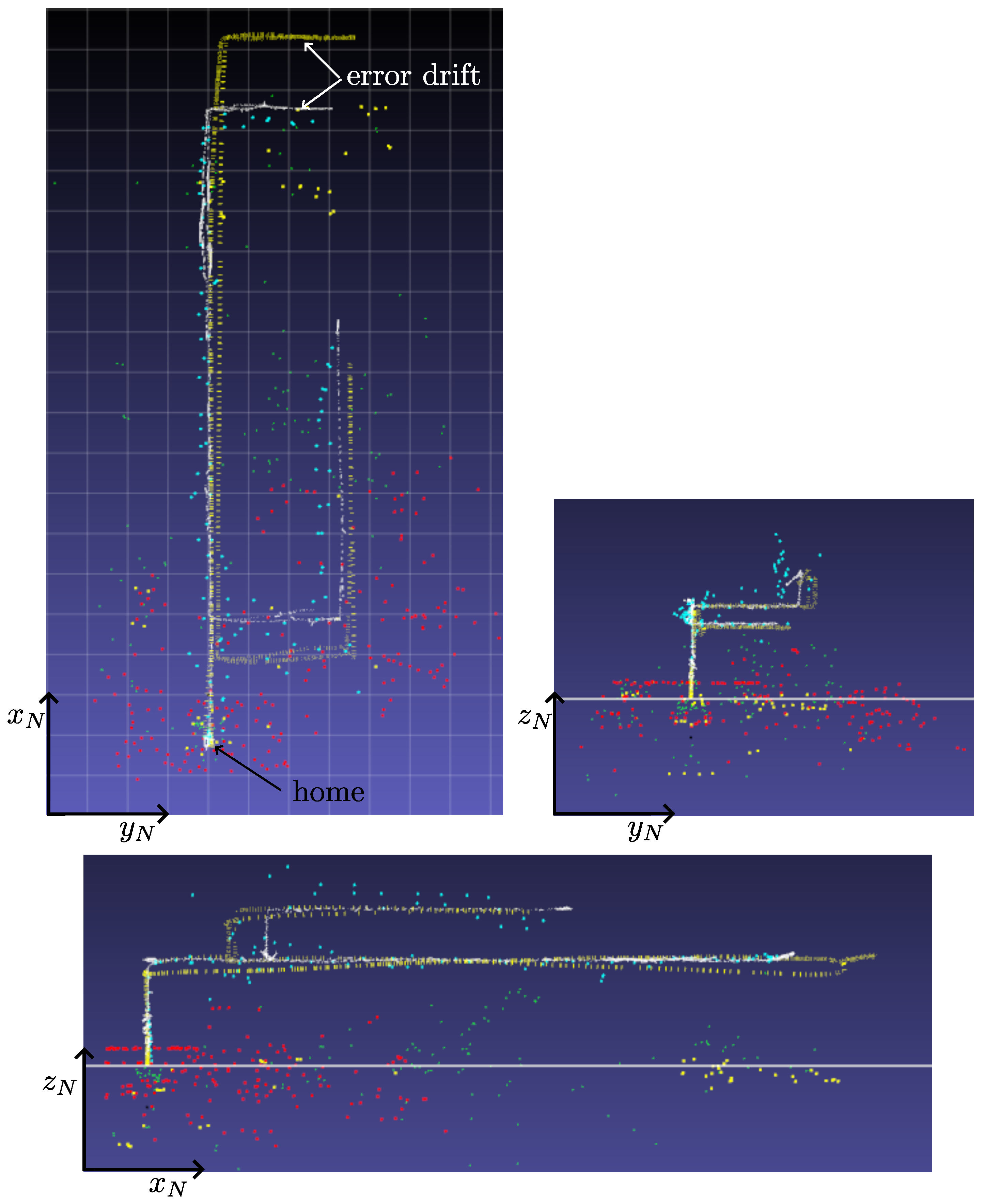
Figure 16 illustrates the estimated flight trajectory and map, along with the actual flight trajectory, presented from the upper (x-y) and lateral (z-y, z-x) views for one of the experiments. As expected, as the UAV moved farther from its home position, some error drift occurred between the estimated and actual flight trajectories, leading to a corresponding drift between the commanded flight trajectory and the actual one. However, despite the error drift, the Go-home command successfully returned the robot to its home position with a precision comparable to that of the previous experiments.

Figure 16. Results obtained from the experiment conducted in the factory-like indoor environment.

6. Conclusions

The results from the virtual experiments indicate that the proposed SCLAM system effectively enables a multi-rotor UAV, equipped with a monocular camera as its primary sensor, to perform fully autonomous exploration missions in GPS-denied environments. These missions include taking off, navigating to a point, exploring the surrounding area, and returning to the home position to land.

Unlike other related methods that focus on evaluating specific estimation-control schemes, this proposal aims to provide a general SCLAM architecture designed to address the challenges of autonomous exploration from a high-level perspective. Importantly, the subsystems within this architecture can be implemented using various control and estimation techniques. For instance, the low-level module could be realized using a predictive control scheme instead. Given the above, it is more appropriate to interpret the virtual experimental results as a validation of a proposed architecture’s viability, rather than an evaluation of a final proposal’s performance.

This does not detract from the fact that the algorithms provided in this work perform reasonably well and can be used to fully implement the proposed architecture. The virtual experiments show that the UAV is able to complete fully autonomous exploration missions. Specifically, the UAV is able to return to its home position with good accuracy, thus minimizing the error drift in the estimated position accumulated during the flight trajectory. The results from virtual experiments in two different GPS-denied environments are presented. Additionally, the computation time statistics validate the real-time performance of the system. The results for the low-level control subsystem, waypoint control subsystem, visual-mark-based control subsystem, and the exploring area algorithm are also presented to validate their expected performance.

Future work could focus on exploring various control, estimation, and trajectory generation techniques for implementing the subsystems within the proposed architecture. This could include the use of alternative control algorithms to enable spiral or circular movements, as well as control methods that produce faster or more aggressive movement responses. While virtual experiments offer valuable insights into the potential performance of the SCLAM system in real-world scenarios, future efforts should also aim to extend these experiments to actual environments, similar to the approach taken with the SLAM subsystem in the author’s previous work.

References

- Smith, J.K.; Jones, L.M. Applications of Unmanned Aerial Vehicles in Surveillance and Reconnaissance. J. Aer. Technol. 2022, 45, 112–125. [Google Scholar]
- Brown, A.R.; White, C.D. Autonomous Navigation and Perception for Unmanned Aerial Vehicles. Int. J. Robot. Autom. 2021, 28, 567–581. [Google Scholar]
- Johnson, P.Q.; Lee, S.H. Challenges in GPS-Dependent Navigation for UAVs in GPS-Denied Environments. J. Navig. Position. 2020, 17, 215–230. [Google Scholar]
- Williams, R.S.; Davis, M.A. Sensor-Based Solutions for UAV Navigation in Challenging Environments. IEEE Trans. Robot. 2023, 39, 78–92. [Google Scholar]
- Anderson, E.T.; Wilson, B.R. Visual Simultaneous Localization and Mapping for UAVs: A Comprehensive Review. Int. J. Comput. Vis. 2022, 50, 321–345. [Google Scholar]
- Anderson, E.T.; Wilson, B.R. Visual-Based SLAM Techniques: A Survey of Recent Advances. IEEE Trans. Robot. 2022, 38, 123–137. [Google Scholar]
- Garcia, M.A.; Patel, S.R. Applications of Visual-Based SLAM in Autonomous Aerial Vehicles. J. Auton. Syst. 2023, 36, 178–192. [Google Scholar]
- Miller, L.H.; Robinson, A.P. Challenges in Real-Time UAV Navigation in Dynamic Environments. IEEE Robot. Autom. Lett. 2021, 26, 4210–4217. [Google Scholar]
- Della Corte, B.; Andreasson, H.; Stoyanov, T.; Grisetti, G. Unified Motion-Based Calibration of Mobile Multi-Sensor Platforms With Time Delay Estimation. IEEE Robot. Autom. Lett. 2019, 4, 902–909. [Google Scholar] [CrossRef]
- Mur-Artal, R.; Tardos, J.D. ORB-SLAM2: An Open-Source SLAM System for Monocular, Stereo, and RGB-D Cameras. IEEE Trans. Robot. 2017, 33, 1255–1262. [Google Scholar] [CrossRef]
- Qin, T.; Li, P.; Shen, S. VINS-Mono: A Robust and Versatile Monocular Visual-Inertial State Estimator. IEEE Trans. Robot. 2018, 34, 1004–1020. [Google Scholar] [CrossRef]
- Shan, T.; Englot, B. LIO-SAM: Tightly-Coupled Lidar Inertial Odometry via Smoothing and Mapping. In Proceedings of the 2020 IEEE/RSJ International Conference on Intelligent Robots and Systems (IROS), Las Vegas, NV, USA, 24 October 2020–24 January 2021; pp. 5135–5142. [Google Scholar]
- Kumar, P.; Zhang, H. Real-time Loop Closure for UAVs in GPS-denied Environments. Auton. Robot. 2023, 59, 49–63. [Google Scholar]
- Shen, S.; Michael, N.; Kumar, V. Tightly-coupled monocular visual-inertial fusion for autonomous flight of rotorcraft MAVs. In Proceedings of the 2015 IEEE International Conference on Robotics and Automation (ICRA), Seattle, WA, USA, 26–30 May 2015; IEEE: Piscataway, NJ, USA, 2015; pp. 5303–5310. [Google Scholar]
- Forster, C.; Pizzoli, M.; Scaramuzza, D. SVO: Fast semi-direct monocular visual odometry. In Proceedings of the 2014 IEEE International Conference on Robotics and Automation (ICRA), Hong Kong, China, 31 May–7 June 2014; IEEE: Piscataway, NJ, USA, 2014; pp. 15–22. [Google Scholar]
- Zhang, Y.; Scaramuzza, D. Model Predictive Control for UAVs with Integrated Visual SLAM. In Proceedings of the 2018 IEEE International Conference on Robotics and Automation (ICRA), Brisbane, Australia, 21–25 May; IEEE: Piscataway, NJ, USA, 2018; pp. 1731–1738. [Google Scholar]
- Faessler, M.; Kaufmann, E.; Scaramuzza, D. Differential flatness-based control of quadrotors for aggressive trajectories. In Proceedings of the 2017 IEEE/RSJ International Conference on Intelligent Robots and Systems (IROS), Vancouver, BC, Canada, 1–24 September 2017; IEEE: Piscataway, NJ, USA, 2017; pp. 5729–5736. [Google Scholar]
- Li, M.; Kim, B.; Mourikis, A. Real-time monocular SLAM for MAVs with improved map maintenance. In Proceedings of the 2016 IEEE/RSJ International Conference on Intelligent Robots and Systems (IROS), Daejeon, Republic of Korea, 9–14 October 2016; IEEE: Piscataway, NJ, USA, 2016; pp. 1764–1771. [Google Scholar]
- Mei, J.; Huang, S.; Wang, D.; Mei, X.; Li, J. Robust outdoor visual SLAM and control for UAVs. In Proceedings of the 2017 IEEE International Conference on Robotics and Automation (ICRA), Singapore, 29 May–3 June 2017; IEEE: Piscataway, NJ, USA, 2017; pp. 6493–6499. [Google Scholar]
- Liu, S.; Lu, L.; Yang, Y.; Wang, H.; Xie, L. Visual SLAM and adaptive control for UAVs in dynamic environments. In Proceedings of the 2019 IEEE International Conference on Robotics and Automation (ICRA), Montreal, QC, Canada, 20–24 May 2019; IEEE: Piscataway, NJ, USA, 2019; pp. 5633–5639. [Google Scholar]
- Kaufmann, E.; Loquercio, A.; Ranftl, R.; Dosovitskiy, A.; Koltun, V.; Scaramuzza, D. Deep Drone Acrobatics. IEEE Robot. Autom. Lett. 2020, 38, 23–31. [Google Scholar]
- Bachrach, A.; Prentice, S.; He, R.; Henry, P.; Huang, A.; Krainin, M.; Maturana, D.; Fox, D.; Roy, N. Estimation, Planning, and Mapping for Autonomous Flight Using an RGB-D Camera in GPS-Denied Environments. Int. J. Robot. Res. 2012, 31, 1320–1343. [Google Scholar] [CrossRef]
- Sun, Y.; Ho, Y.S.; Qian, C.; Shao, L.; Zhang, H. Reinforcement learning-based visual SLAM for autonomous UAV navigation. In Proceedings of the 2018 IEEE International Conference on Robotics and Automation (ICRA), Brisbane, Australia, 21–25 May 2018; IEEE: Piscataway, NJ, USA, 2018; pp. 2402–2409. [Google Scholar]
- Munguía, R.; Trujillo, J.C.; Obregón-Pulido, G.; Aldana, C.I. Monocular-Based SLAM for Mobile Robots: Filtering-Optimization Hybrid Approach. J. Intell. Robot. Syst. 2023, 109, 53. [Google Scholar] [CrossRef]
- SLAM Source Code. Available online: https://github.com/rodrigo-munguia/Hybrid_VSLAM (accessed on 17 January 2025).
- Wu, Y.; Hu, Z. PnP Problem Revisited. J. Math. Imaging Vis. 2006, 24, 131–141. [Google Scholar] [CrossRef]
- Itseez. Open Source Computer Vision Library. 2015. Available online: https://github.com/itseez/opencv (accessed on 17 January 2025).
- Macenski, S.; Foote, T.; Gerkey, B.; Lalancette, C.; Woodall, W. Robot Operating System 2: Design, architecture, and uses in the wild. Sci. Robot. 2022, 7, eabm6074. [Google Scholar] [CrossRef] [PubMed]
- Webots: Mobile Robot Simulation Software. Available online: https://cyberbotics.com/ (accessed on 17 January 2025).
- SCLAM Source Code. Available online: https://github.com/rodrigo-munguia/SCLAM-UAVs (accessed on 17 January 2025).
Disclaimer/Publisher’s Note: The statements, opinions and data contained in all publications are solely those of the individual author(s) and contributor(s) and not of MDPI and/or the editor(s). MDPI and/or the editor(s) disclaim responsibility for any injury to people or property resulting from any ideas, methods, instructions or products referred to in the content. |
© 2025 by the authors. Licensee MDPI, Basel, Switzerland. This article is an open access article distributed under the terms and conditions of the Creative Commons Attribution (CC BY) license (https://creativecommons.org/licenses/by/4.0/).