Co-Registration of Multi-Modal UAS Pushbroom Imaging Spectroscopy and RGB Imagery Using Optical Flow

Abstract

Remote sensing from unoccupied aerial systems (UASs) has witnessed exponential growth. The increasing use of imaging spectroscopy sensors and RGB cameras on UAS platforms demands accurate, cross-comparable multi-sensor data. Inherent errors during image capture or processing can introduce spatial offsets, diminishing spatial accuracy and hindering cross-comparison and change detection analysis. To address this, we demonstrate the use of an optical flow algorithm, eFOLKI, for co-registering imagery from two pushbroom imaging spectroscopy sensors (VNIR and NIR/SWIR) to an RGB orthomosaic. Our study focuses on two ecologically diverse vegetative sites in Tasmania, Australia. Both sites are structurally complex, posing challenging datasets for co-registration algorithms with initial georectification spatial errors of up to 9 m planimetrically. The optical flow co-registration significantly improved the spatial accuracy of the imaging spectroscopy relative to the RGB orthomosaic. After co-registration, spatial alignment errors were greatly improved, with RMSE and MAE values of less than 13 cm for the higher-spatial-resolution dataset and less than 33 cm for the lower resolution dataset, corresponding to only 2–4 pixels in both cases. These results demonstrate the efficacy of optical flow co-registration in reducing spatial discrepancies between multi-sensor UAS datasets, enhancing accuracy and alignment to enable robust environmental monitoring.

1. Introduction

1.1. Background

Recent advancements in UAS technology and their adoption within the remote sensing community have enabled mapping at significantly higher spatial resolutions compared to other airborne or spaceborne techniques, while also providing larger spatial coverage than traditional field sampling methods [1,2]. With the development of small and lightweight imaging spectroscopy sensors, also referred to as hyperspectral sensors, there are increasing opportunities for high-spatial-resolution and high-spectral-resolution data acquisitions from UASs, facilitating new discoveries in a range of domains. Imaging spectrometers can measure surface reflectance across a range of wavelengths in the electromagnetic (EM) spectrum. These measurements have been used to predict various plant biophysical and biochemical traits, as well as biodiversity metrics such as plant functional diversity and species composition from UASs and other airborne platforms (e.g., [3,4,5,6]). Beyond the study of ecological systems, UAS imaging spectroscopy is being increasingly utilised across a range of industries, including agricultural [7,8], and geological applications [9,10]. Given the modular nature of UAS platforms, payload weight and size limitations often necessitate the use of smaller, specialised sensors or multiple flights with different imaging spectrometers. As a result, imaging spectroscopy data are often collected across multiple flight instances. This modular approach enables flexible and cost-effective data acquisition but also introduces challenges in ensuring spatial alignment across datasets. As the use of these sensors grow across various research and industry sectors, there is an increasing need for spatially accurate and cross-comparable imagery to ensure their reliability and applicability.

For imaging spectrometers, there is a specific processing workflow to get from raw imagery to surface reflectance imagery (see refs. [1,11,12,13]). One of the key steps in this workflow, specifically for pushbroom imaging spectroscopy data, is georectification. Pushbroom sensors utilise a line scanning technique in which an orthogonal line of spatial samples are measured simultaneously with the spectral samples at every trigger [14,15]. A pushbroom sensor requires forward motion to build a spatial scene. In motion, distortions of local line scans within the imagery can occur with pose changes of the platform. Georectification corrects for any geometric distortions, primarily through synchronising the platform’s attitude (roll, pitch, and yaw) movements and position (easting, northing, height) with the individual line scans from the sensor (see [16,17,18]). Accurate estimations of the sensor’s position and attitude need to be obtained simultaneously to the data acquisition and are performed through an on-board inertial navigation system (INS) containing a GNSS receiver and inertial measurement unit (IMU). The accuracy, quality, and synchronisation of the INS measurements alongside precise measurements of any lever arm and boresight offsets are key for accurate georectification of pushbroom imagery [16,19]. Additionally, projecting the image pixels onto a surface as part of the orthorectification process requires an accurate digital elevation model (DEM) or digital surface model (DSM) [20]. Inaccuracies in the measurement or processing of INS data and the DEM/DSM can lead to spatial misalignment. Given the unique nature of pushbroom scanning, these spatial offsets can occur both locally, at the pixel or groups of pixels level, and globally, affecting an entire flight line or mosaic scene. Such misalignments can significantly hinder cross-comparisons across different datasets and sensor payloads, affecting the reliability of the imagery. This highlights the need for techniques to ensure accurate spatial alignment, crucial for obtaining reliable and accurate imagery for effective environmental monitoring and other remote sensing applications.

1.2. Related Works

To correct for misalignments between sets of imagery, different co-registration techniques have been proposed in past research. Registration between remotely sensed imaging spectroscopy and RGB imagery has been investigated using feature detection and matching based on algorithms such as the scale invariant feature transform (SIFT) or speeded up robust features (SURF) and their adaptations [17,21,22,23,24]. In their study, Angel, et al. [17] achieved centimetre- to decimetre-level co-registration of UAS pushbroom imaging spectroscopy and RGB imagery using SURF and the maximum likelihood estimator sample consensus (MLESAC) to fit the best geometric model based on the identified features. These results were further supported by Finn, et al. [23]. However, feature detection and matching algorithms work best when the imagery has distinct geometric features but can struggle to find and match features in more complex environments, such as forests. Additionally, by identifying only specific features in the imagery, these algorithms can only approximate the underlying deformation of individual pixels.

Deep learning frameworks have been proposed for image-to-image co-registration, particularly in computer vision and medical imaging applications with growing popularity in remote sensing studies [25,26,27,28,29]. Deep learning frameworks for co-registration in remote sensing have primarily focused on imagery obtained from satellite sensors. Algorithms such as convolutional neural networks (CNNs) and their adaptations have been most popular, as well as Siamese networks and generalised adversarial networks (GANs) [28,29]. While deep-learning frameworks show promising results for co-registration, they often require large, labelled datasets for training and can be computationally intensive.

Another method for co-registration is the use of optical flow, a computer vision technique that calculates the motion between consecutive frames of video or images based on the apparent movement of brightness patterns [30]. Optical flow is an algorithm based on non-rigid motion estimation that can compute the displacement of pixels between pairs of images. Optical flow techniques such as the Extended Flow Optical Lucas–Kanade Iterative (eFOLKI) and the Geoscience Extended Flow Optical Lucas–Kanade Iterative (GeFOLKI), both adaptations of the Lucas–Kanade method [31,32], have demonstrated significant potential in the co-registration of satellite imagery [33,34]. Initially applied to SAR imagery, these methods have been extended to a variety of satellite remote sensing datasets, including SAR, optical, and LiDAR imagery. They have proven effective in refining georeferencing accuracy [35,36,37] and have been employed in diverse applications such as quantifying landslide deformation [38], glacier surface velocity extraction [39], and estimating sea-ice flow [40]. Optical flow co-registration has only been tested on satellite based datasets and, for co-registration of high-resolution pushbroom imagery taken from UAS platforms, this technique is appealing due to its ability to account for local displacements whilst also being computationally efficient [33]. However, further testing is needed to evaluate their effectiveness in co-registering high-resolution UAS imagery captured across different regions of the EM spectrum and for geometrically complex datasets, such as those associated with environmental or vegetation monitoring.

Here, we propose the use of the optical flow algorithm eFOLKI to co-register high-resolution pushbroom imaging spectroscopy data across different spectral ranges from VNIR to SWIR and RGB imagery captured at different instances by UAS platforms. A challenging problem in co-registration of UAS imagery, in particular pushbroom imaging spectroscopy, is that the images contain highly localised, non-systematic, non-linear distortions. Furthermore, UAS images are often acquired at slightly different times when one sensor is flown after the other. This results in differences in lighting conditions, shadows, and observation angles. The combination of localised geometric distortions and temporal variability presents a significant challenge for co-registration. The selection of the eFOLKI algorithm for this study was motivated by its ability to handle pixel-level deformations, making it particularly effective in complex environments like native forests, where feature-based methods often struggle. Unlike deep learning approaches, which require large training datasets and significant computational resources, eFOLKI is computationally efficient and does not require prior training. The aim of this study is to provide a first of its kind accuracy assessment of this co-registration method, for imagery taken over diverse and complex natural environments, ensuring features such as trees, shrubs, and grass clumps overlap accurately across discrete UAS-based imagery taken in the visible, near infrared, and short-wave infrared wavelength ranges. Through this assessment, we seek to demonstrate the effectiveness of eFOLKI, supporting future research in co-registration of multi-modal UAS imagery for precise cross-comparison, data fusion, or change detection.

2. Methods

2.1. Study Area

This study focused on two sites that exhibit key natural conservation characteristics and were selected due to their contrasting structural characteristics. The first study site, Cockatoo Hills, is located adjacent to Brady’s Lake in the central highlands of Tasmania, Australia, approximately 100 km to the northwest of Hobart (Figure 1). Cockatoo Hills is home to an expansive sphagnum moss ‘forest’. These sphagnum bogs are nationally protected due to their conservation value [41,42]. Additionally, this site has complex structural components, being located between an open grassland and amongst an open dry eucalypt forest. The second site is located near the Swansea township on the east coast of Tasmania (Figure 1). This site consists of a terrain gradient between the Wye River and Rocky Rivulet and is a dry eucalypt forest home to a diverse mix of key conservation species. The Swansea site has been a focus area for plant hydraulic research [43,44,45] as well as past UAS remote sensing studies [3,46]. UAS flights were undertaken at the Cockatoo Hills study site on the 15 December 2021 and at the Swansea site on the 18 February 2021. The UAS flights covered an approximate area of 1.56 hectares at Cockatoo Hills and 10.2 hectares at Swansea. Both sites were flown during low-wind and sunny conditions, within an hour of solar noon.

2.2. UAS Platforms and Data Acquisition

The UAS platform used for the acquisition of imaging spectroscopy data in this study was the DJI Matrice 600 (DJI, Shenzhen, China). The Matrice 600 was equipped with a modular payload system (Figure 1) consisting of the imaging spectroscopy sensor, an INS (Spatial Dual, Advanced Navigation, Sydney, NSW, Australia), as well as an on-board computer (NUC, Intel, Santa Clara, CA, USA) with an in-built data synchronisation unit. The Spatial Dual and the imaging spectroscopy sensor were attached to the Matrice 600 via a stabilising nadir-viewing gimbal, the DJI Ronin MX. This payload was designed to be modular, allowing for the swapping of imaging spectroscopy sensors and, in this study, two sensors were flown consecutively. Both sensors were manufactured by Specim (Specim, Oulu, Finland), the FX10 measuring in the VNIR range of the EM spectrum (400–1000 nm) and the FX17, measuring in the NIR to SWIR region of the spectrum (900–1700 nm). Both sensors captured 224 spectral bands with the FX10 having an average full width at half maximum (FWHM) of 5.5 nm and the FX17 having an average FWHM of 8 nm. The synchronisation unit (Adept Turnkey, Perth, Australia) allowed for direct georeferencing of the imagery through providing position and attitude timestamps from the INS. The system was intentionally designed to be modular, allowing for the regular swapping and deployment of the VNIR and NIR/SWIR sensors. Lever arm offsets (X, Y, and Z distance between primary GNSS antenna and the phase centre of the INS) were measured with millimetre precision. For data acquisition, the sensors were flown in parallel, 30% overlapping flight lines. At Cockatoo Hills, the flights were flown at a height of 40 m and a speed of 3.0 m/s, resulting in a spatial resolution of ~4 cm. At Swansea, the UAS was flown at a height of 90 m and a speed of 4.0 m/s, resulting in a spatial resolution of ~8 cm.

RGB imagery was additionally collected at both study sites. At Cockatoo Hills, the UAS platform for RGB capture was the DJI Matrice 300 with a DJI Zenmuse P1 45-megapixel full-frame sensor and 35 mm lens. At the Swansea study site, the RGB imagery was collected with a DJI Phantom 4 pro version 2 with a gimballed 1 inch 20 MP CMOS sensor. For accurate georeferencing of the RGB imagery, ground control points (GCPs) were laid out across both study sites. The GCPs were distributed to provide uniform coverage across both study sites, ensuring all areas were represented in the georeferencing process. Placement accounted for variations in topography and areas of interest. Accessibility and visibility of GCPs in the imagery were prioritised to ensure accurate identification during processing. The placement of 12 GCPs at Cockatoo Hills (~1.5 ha) and 21 at Swansea (~10.2 ha) ensured adequate coverage and control for accurate georeferencing across each site. The coordinates of the GCPs were collected with a Leica GS14 rover, receiving real-time kinematic (RTK) corrections from a GS14 base over a known point. The reference coordinate for the base station was retrieved from AUSPOS [47] using observations collected over the point across a duration of six hours. The RGB imagery was similarly flown with parallel, overlapping flight lines and resulted in a spatial resolution of ~1 cm for the Cockatoo Hills RGB imagery (flying height and speed of 80 m and 3 m/s) and ~3 cm for the Swansea imagery (flying height 90 m and speed 5 m/s).

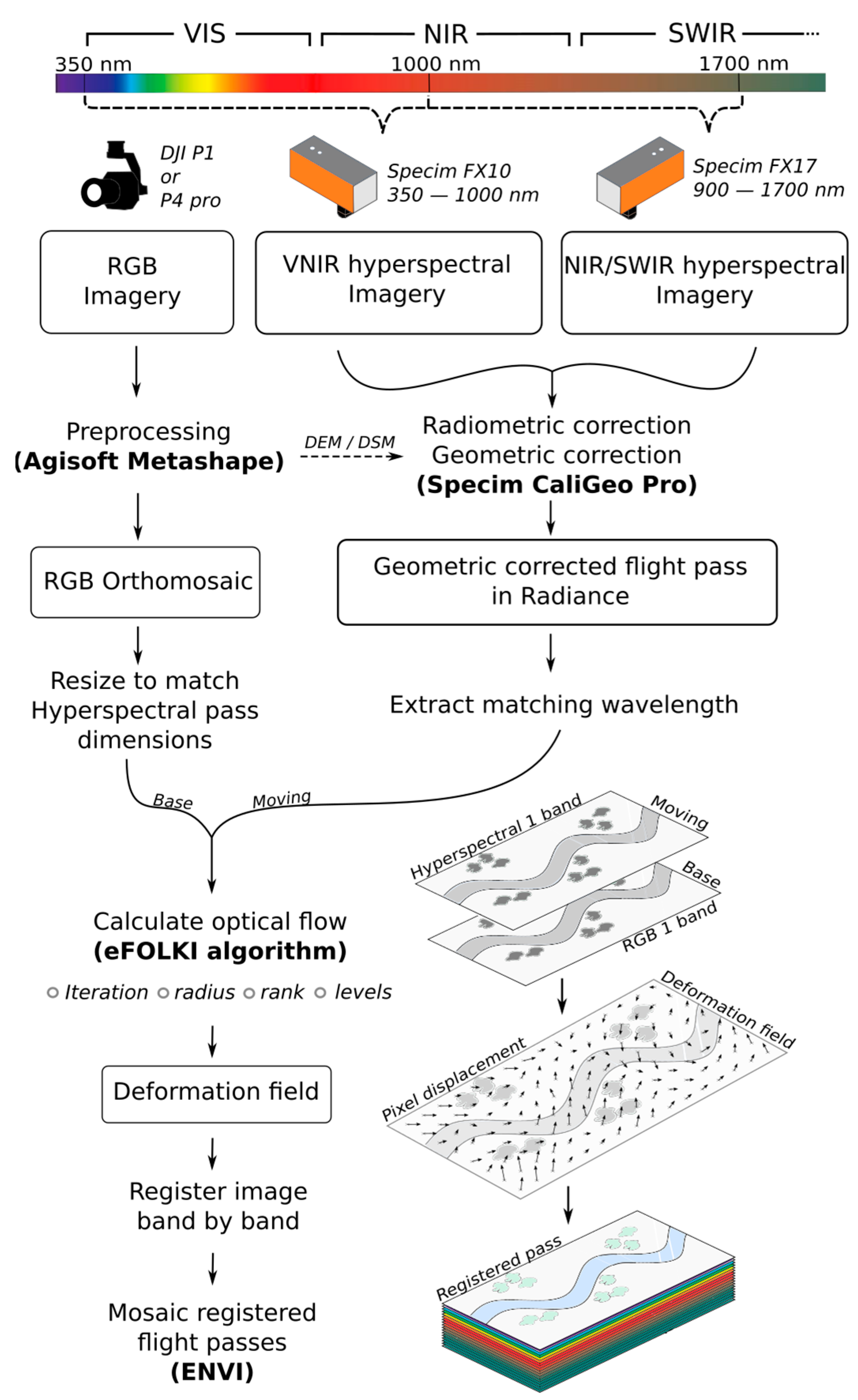
2.3. Imagery Pre-Processing

2.3.1. RGB Imagery

The RGB imagery collected from both study sites was processed in Agisoft Metashape, version 2.0.1 [48]. The imagery was aligned before being accurately georeferenced using the GCP coordinates. Through using independently measured GCPs, receiving corrections from a processed known point (see Section 2.2), the absolute accuracy of the georectified RGB imagery was high (~2–4 cm). A dense point cloud was created from the aligned imagery to facilitate the processing of a digital elevation model (DEM) and digital surface model (DSM). For the Cockatoo Hills dataset, a ground-based DEM was created and used for the projection of the RGB imagery. This was due to the site primarily including ground vegetation (sphagnum moss and grassland) with minimal tree coverage. This was achieved by using the classify point cloud tool in Metashape and creating a DEM based on the ground classified points (settings for classification: max angle: 15, max distance: 0.2, cell size: 20, erosion radius: 0). A ground-based DEM was additionally tested with the Swansea dataset. Due to the higher tree cover and greater structural complexity at the Swansea site (Figure 1), ground points were sparse, resulting in a less accurate DEM. Therefore, a DSM was created in Metashape based on a smoothed mesh (smoothing level: 100) from the tie points (or sparse point cloud) to represent the surface height of the vegetation.

2.3.2. Imaging Spectroscopy

The imaging spectroscopy data collected by both the Specim FX10 and FX17 (hereon referred to as VNIR and NIR/SWIR) were radiometrically and geometrically corrected using Specim software CaliGeo Pro (Version 2.6.1) [49]. To reduce variability caused by the view angles of the sensors, the edges of the flight strips were cropped whilst retaining the central portion and ensuring minimal overlap between adjacent flight strips. Depending on the imagery and underlying terrain, the flight strips were cropped by between 10–15% on both edges, retaining the central 70–80% of the imagery. This step was taken to optimise the overlap of flight strips along the edges and to reduce edge effects (both FX10 and FX17 cameras have a 38° field-of-view). This imagery was then converted to at-sensor radiance with radiometric calibration factors before undergoing georectification. For radiometric correction, factory calibration data provided by Specim were used to convert pixel values from raw digital numbers to radiance. Dark current imagery was taken following each flight to subtract for background noise per pixel. For georectification, high-accuracy post-processed INS data were generated with Kinematica [50], using the on-board Spatial Dual as the rover and a Leica GS14 over the known point as the base reference. Time synchronisation data from the INS were used in CaliGeo Pro to georectify the imagery line by line, correcting for attitudinal distortions caused by the movement of the UAS platform. Finally, the imagery was projected on to the DEM or DSM as described in Section 2.3.1 to produce georectified flight passes in (W m⁻² μm⁻¹ sr⁻¹).

2.4. Co-Registration

2.4.1. Algorithm Description

The optical flow algorithm used in this study is the Extended Flow Optical Lucas–Kanade Iterative, eFOLKI, developed by Plyer, et al. [51]. eFOLKI is an adaptation of the FOLKI algorithm developed by Le Besnerais and Champagnat [32], initially inspired by the Lucas–Kanade optical flow algorithm [31]. A further adaptation of eFOLKI is Geoscience Extended Flow Optical Lucas–Kanade Iterative (GeFOLKI) by Brigot, et al. [33]. GeFOLKI was adapted for the co-registration of heterogeneous imagery, such as synthetic aperture radar (SAR) to optical imagery, through performing a contrast inversion. Due to the imagery presented in this study being moderately homogenous with little contrast difference, the eFOLKI algorithm was chosen. eFOLKI is a dense and non-parametric co-registration method, computing the displacement for every pixel between a set of images. The algorithm uses a local or window-based approach to estimate flow at each pixel by minimising a criterion (in this case, intensity differences) through an iterative Gauss–Newton strategy based on the first-order Taylor expansion of image intensity [34,51]. In simple terms, it estimates the displacement of a pixel by looking at a small surrounding area and repeatedly adjusting its estimate to minimise differences in brightness. Through repeatedly adjusting its estimates, the eFOLKI algorithm is iterative, and it is also multi-resolution, meaning it uses a pyramid of images at different scales to refine the displacement estimates from coarse to fine detail, with iteratively varying windows sizes at each pyramid level [34]. A rank transform is additionally computed prior to minimisation to highly compress the signal dynamics, enhancing the robustness of the displacement estimates. The output from this algorithm is a deformation field that is used to co-register the pairs of images.

2.4.2. Workflow

The eFOLKI algorithm was implemented using the Python programming language (version 3.10) using code supplied by the authors [52]. Inputs for the eFOLKI algorithm require the imagery to be of the same X, Y, and Z dimensions. Figure 2 shows the general workflow with a subset of the RGB orthomosaic to match the extent of the individual passes of the hyperspectral imagery. It was then further resized to match the dimensions of the hyperspectral pass (same width and height). As the imagery had to have the same Z dimension (spectral dimension), single band inputs were used for the co-registration. From the RGB imagery, the green band was used for matching due to the high signal from vegetation. From the VNIR imagery, wavelength 551 nm was used for matching, as it corresponds to the green wavelength. As the NIR/SWIR imagery did not overlap the visible region of the spectrum, through experimentation, wavelength 1106 nm was chosen for matching against the RGB image. Other inputs were tested, such as calculated vegetation indices (VIs) or wavelength sums, but were not used as they did not significantly advance the registration result when compared to the less complex single-band input. An additional experiment was conducted for the Swansea dataset where the NIR/SWIR imagery was directly co-registered to the VNIR imagery. This was performed by co-registering between the overlapping wavelength at 970 nm, which was chosen due to the quality of the signal at this wavelength, showing little noise. The eFOLKI algorithm created a deformation field, which was used to register the image pairs. After all passes were registered, they were mosaiced using the seamless mosaic tool in ENVI version 5.6 [53].

2.4.3. Parameter Selection

Overall, there are four adaptable parameters when tuning the eFOLKI algorithm: the number of iterations per level (iteration), the windows radius (radius), the size of the rank transform (rank), and the number of pyramid levels (levels). These parameters were adjusted based on the characteristics of the individual pass and can be seen in Table S1 (Supplementary Materials). As explained in Brigot, et al. [33], if the displacement estimate is greater than several tens of pixels, a higher pyramid level is needed. Due to relatively large displacements in this study, a pyramid level of 6 was chosen and kept constant across all co-registrations. Similar to the findings by Charrier, et al. [40], through experimentation a rank value of 4 was found to be most appropriate across all co-registrations. The radius and iteration parameters were found to be key for accurate alignment and were adjusted per pass (Table S1). The radius was tested iteratively, in steps of 4, with the most effective being the combination of 16, 8, and 4. Iteration values of 8 were found to be most effective but between certain image pairs it was tested in steps of 8 with a maximum value of 32.

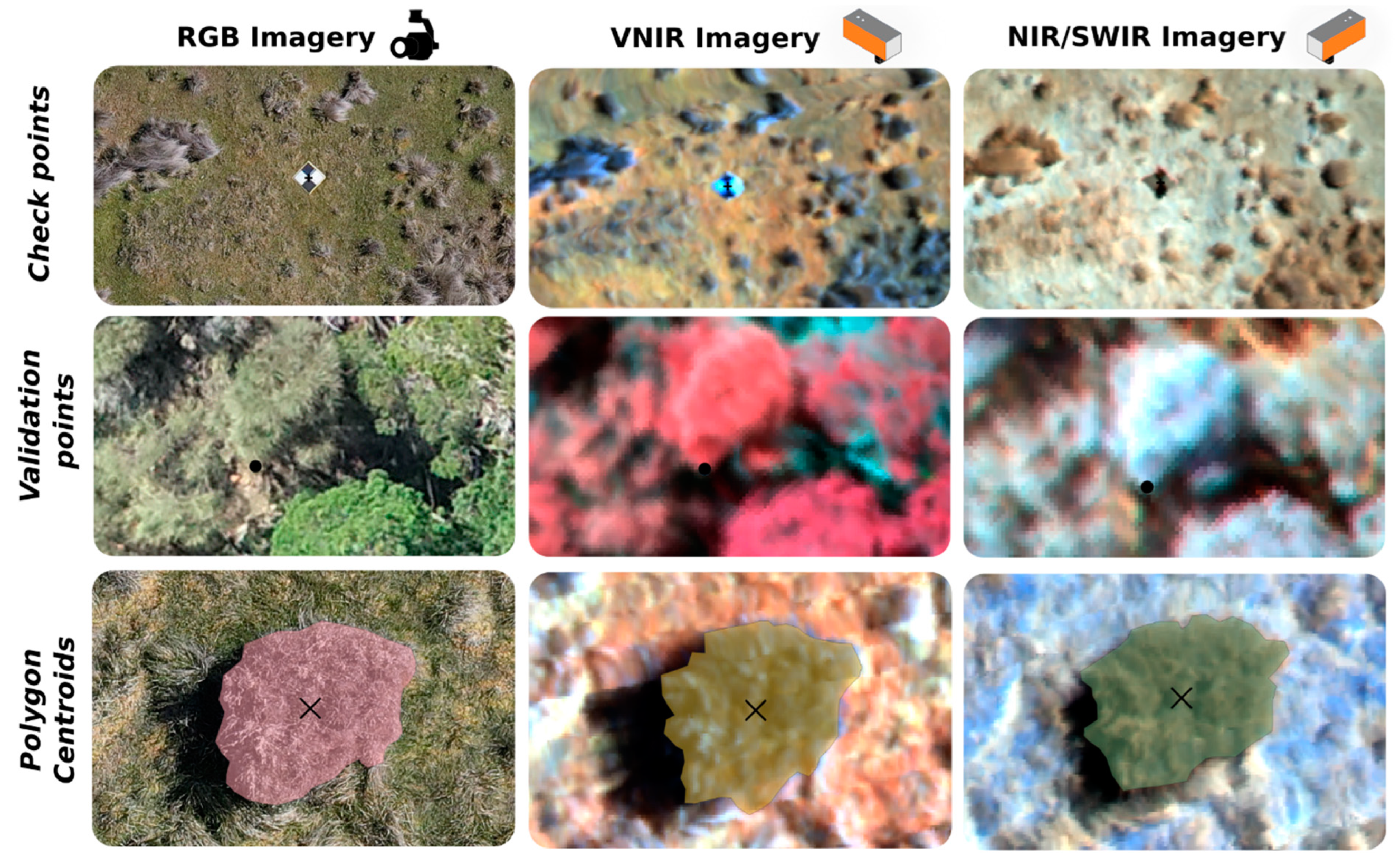
2.5. Accuracy Assessment

An initial assessment of the performance and guidance of eFOLKI parameter selection was first evaluated visually. Visual assessment was conducted in QGIS (version 3.22) using the map swipe tool plugin. To quantitively assess the quality of the co-registration accuracy, the following metrics where chosen.

i.

Check points and validation points

GCPs were placed throughout both study sites to allow for accurate georeferencing of the RGB imagery against independently measured and clearly identifiable verification targets. Due to the high spatial resolution of the imaging spectroscopy acquired at the Cockatoo Hills study site, these GCPs were able to be used as check points to assess the accuracy of the co-registration. The imaging spectroscopy acquired at Swansea had a lower spatial resolution and thus the on-ground GCPs were unable to be accurately identified. Therefore, validation points were used to assess the co-registration accuracy. Validation points were determined as clear points that were able to be identified in all sets of imagery. Examples of these validation points included edges of tree crowns, ends of branches, or sharp edges of large rocks (Figure 3). Overall, there were 12 GCPs used as check points for the Cockatoo Hills dataset, with an additional 12 validation points being identified (24 points in total). For the Swansea dataset, 24 validation points were identified for accuracy assessment.

ii.

Polygon centroids

A primary objective of this study is to align multi-sensor imagery to enhance cross-comparison and change detection for ecosystem monitoring, ensuring that features like trees, shrubs, and grass clumps are accurately co-registered. Therefore, additional metrics were identified based on the centre point of digitised polygons in the imagery (Figure 3). Twelve trees, shrubs, or grass clumps were identified and digitised in the Cockatoo Hills imagery as polygons. Predominantly trees were identified in the Swansea dataset, resulting in the creation of 24 polygons. The distribution of check points, validation points, and polygons for both study sites is shown in Figure S1.

The locations of the check points, validation points, and features used to create polygons were strategically selected to ensure even spatial distribution across the entire study area, for both study sites. This approach ensured the diverse land cover types and terrain variations present at both sites were represented for the accuracy assessment. The distribution of these points at both study sites is shown in Figure S1.

Performance Metrics

i.

Error quantification

Using the validation points, check points (in the Cockatoo Hills imagery), and shape centroids, the Euclidian distances between these points in the VNIR and NIR/SWIR imagery and the points in the RGB imagery were calculated (Equation (1)). The points located in the RGB imagery were used as the observed or known value, due to their high absolute accuracy, and the points from the imaging spectroscopy were used as the predicted values.

$$D_{p-o}=\sqrt{{{(X}_p-X_o)}^2+{{(Y}_p-Y_o)}^2}$$

(1)

where D_{p – o} represents the distance between the predicted values (p) and the observed values (o).

Two metrics were used to assess the accuracy of these points based on their Euclidian distance to the observed value (RGB imagery): the root mean square error (RMSE), calculated using Equation (2), and the mean absolute error (MAE), calculated using Equation (3). Additionally, these metrics were calculated for both datasets where the observed point was in the VNIR imagery and the predicted value in the NIR/SWIR imagery to check the co-registration accuracy between the two sensors.

$$\mathrm{R}\mathrm{M}\mathrm{S}\mathrm{E}=\sqrt{{\displaystyle \frac{{\sum }_{i=1}^n{\left(D_{p-o}\right)}^2}{n}}}$$

(2)

$$\mathrm{M}\mathrm{A}\mathrm{E}={\displaystyle \frac{\sum _{j=1}^n{D}_{p-o}}{n}}$$

(3)

ii.

Intersection over union

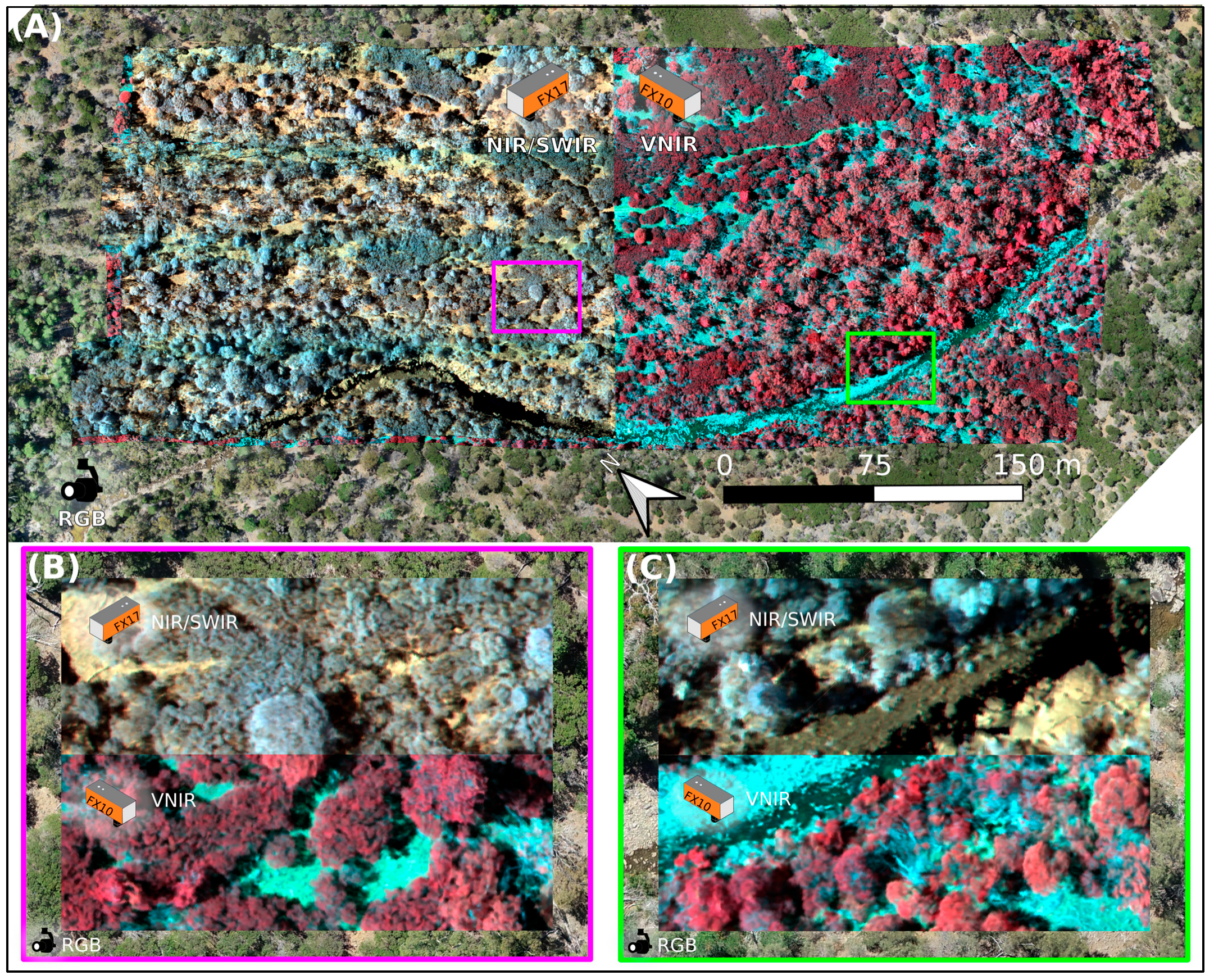
A valuable metric for evaluating differences between polygons derived from different images is the intersection over union (IoU). IoU measures the overlap between polygons by dividing the intersecting area by the total combined area of the shapes. This metric has been shown to be suitable for assessing the performance of segmentation and object detection algorithms [46,54], producing values within a closed range from 0 to 1. Using the polygons identified in the previous section, IoU was calculated between all polygons from the different sets of imagery, resulting in 12 IoU values for Cockatoo Hills and 24 IoU values for the Swansea dataset.

3. Results

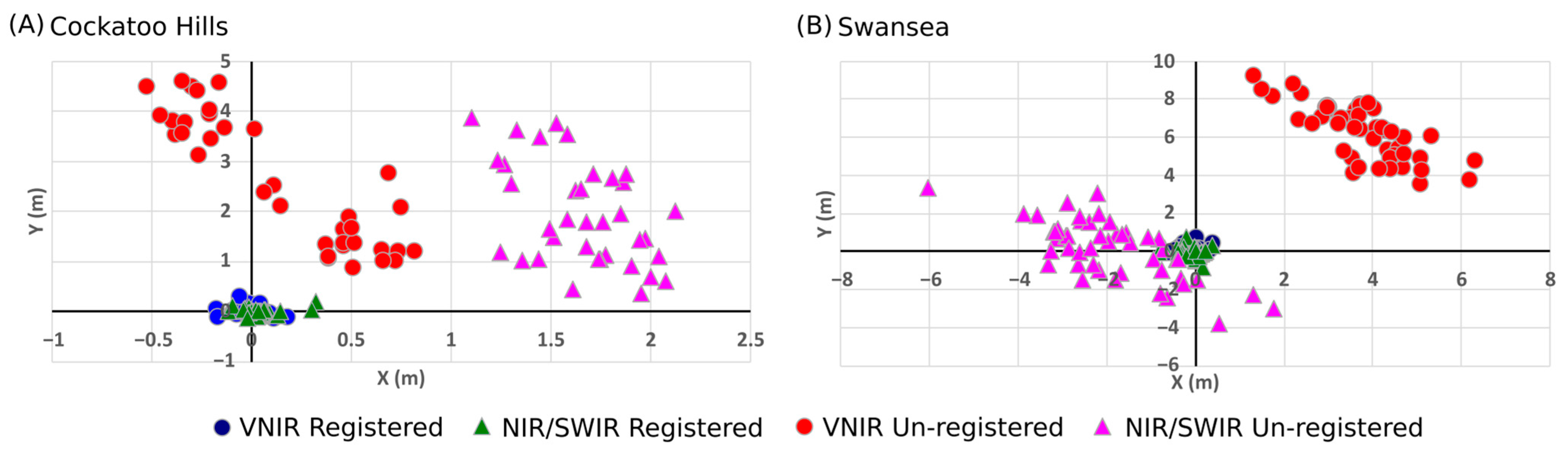
3.1. Optical Flow Results

3.1.1. Cockatoo Hills

A visual assessment of the co-registration for the Cockatoo Hills dataset indicated a high degree of spatial alignment (Figure 4 and Video S1). This initial visual evaluation is important to assess any offsets between the sets of imagery, especially in areas that may not be covered by check points, validation points, or polygons. Visual co-registration errors were minimal, particularly in the areas of grassland or ground cover. Relatively small shifts were observed in the taller tree crowns. The efficiency of the algorithm to calculate optical flow was high with an average time of less than 1.52 min in the Cockatoo Hills image pairs, using a laptop of moderate computing power (Table S2).

3.1.2. Swansea

Visual assessment of the co-registration for the Swansea imagery similarly showed a high degree of alignment (Figure 5 and Video S2). Figure 5 shows the results where the VNIR imagery was co-registered to the green band from the RGB imagery, and the NIR/SWIR imagery was directly co-registered to the already corrected VNIR imagery via an overlapping wavelength. Figure 5B,C show good alignment at the local level for both sets of imagery. The larger array sizes for the Swansea imagery resulted in greater processing times, increasing to an average of 13.48 min for the VNIR calculations and 6.91 min for the NIR/SWIR (Table S2).

3.2. Accuracy Assessment Results

3.2.1. Error Quantification

In the Cockatoo Hills dataset, prior to co-registration the RMSE and MAE values in the un-registered imagery were up to 2.931 m and 2.660 m, respectively. This heavily improved with the registration between the VNIR imagery (wavelength 551 nm) and RGB imagery (green band), achieving the lowest RMSE and MAE of 0.103 m and 0.080 m, respectively, equivalent to 2–3 pixels (

Table 1. RMSE and MAE values for the un-registered and co-registered passes at both study sites. RMSE, Root Mean Square Error; MAE, Mean Absolute Error; RGB, Red Green Blue; VNIR, Visible Near-Infrared; NIR, Near-Infrared; SWIR; Short-Wave Infrared.

					Un-Registered		Registered
Site		Imagery	Reference	Total Points	RMSE (m)	MAE (m)	RMSE (m)	MAE (m)
Cockatoo Hills		VNIR	RGB	36	2.931	2.660	0.103	0.080
		NIR/SWIR	RGB	36	2.749	2.660	0.110	0.083
		NIR/SWIR	VNIR	36	2.238	2.043	0.129	0.092
Swansea		VNIR	RGB	48	7.534	7.481	0.243	0.186
		NIR/SWIR	RGB	48	2.797	2.563	0.321	0.246
		NIR/SWIR	VNIR	48	8.730	8.656	0.221	0.168

). The registration of the NIR/SWIR (wavelength 1106 nm) to the RGB imagery was only slightly different with RMSE and MAE values of 0.110 m and 0.083 m after co-registration. The alignment between the VNIR and NIR/SWIR imagery after co-registration was also high, with RMSE and MAE values of 0.129 m and 0.092 m, respectively, improving from 2.238 m and 2.043 m in the un-registered imagery. Out of the points used for accuracy assessment (check points, validation points, and shape centroids), the check points identified from the on-ground GCPs in the Cockatoo Hills imagery held the lowest error after co-registration with <0.05 m RMSE and MAE (Table S3).

For the Swansea dataset, prior to co-registration, the spatial inaccuracy was high with the errors between the un-registered NIR/SWIR and VNIR imagery having the highest spatial offset, yielding RMSE and MAE values of 8.730 m and 8.656 m, respectively. Co-registration significantly improved these errors with the best results being based on imagery projected onto the smoothed DSM and building the optical flow between the VNIR data and the green band from the RGB imagery. The NIR/SWIR imagery was directly co-registered to the already corrected VNIR imagery, using wavelength 970 nm from both sets of imagery. The registration between the NIR/SWIR and VNIR imagery showed the greatest improvement with RMSE and MAE results of 0.221 m and 0.168 m, respectively, equivalent to a spatial offset of 2–3 pixels (Table 1). With the RGB imagery as reference, the registered VNIR imagery yielded similar RMSE and MAE values of 0.243 m and 0.186 m, respectively. The NIR/SWIR registration produced slightly higher RMSE and MAE values of 0.321 m and 0.246 m, equivalent to 3–4 pixels. Co-registration between the VNIR and RGB imagery using the ground-based DEM resulted in higher errors compared to the co-registrations using the smoothed canopy-based DSM, with RMSE and MAE values of 0.339 m and 0.248 m after co-registration using the DEM projected imagery (Table S3). The smoothed DSM did not significantly improve the co-registration alignment for the NIR/SWIR imagery compared to using the DEM. However, registering the NIR/SWIR directly to the VNIR imagery using the overlapping wavelength highly improved the co-registration accuracy. The co-registration between the NIR/SWIR imagery and the green band of the RGB imagery resulted in relatively high errors, with RMSE and MAE values of 1.153 m and 0.876 m, respectively (Table S3).

The difference in the X and Y horizontal coordinates between the un-registered and co-registered imagery is shown in Figure 6. The Swansea dataset held the highest original planimetric errors in the un-registered imagery of up to 9.2 m. These initial errors were higher in the VNIR imagery than the NIR/SWIR imagery, with the NIR/SWIR imagery having a maximum offset of 6 m. After co-registration these offsets were improved to a maximum of 0.76 m in the Y and 0.43 m in the X. The Cockatoo Hills datasets held lower original spatial offsets compared to the Swansea dataset, with a maximum planimetric distance of 4.6 m (Figure 6A). The offsets in the un-registered VNIR imagery were more spread than in the NIR/SWIR with the NIR/SWIR imagery having the highest offset in the X direction (2.12 m). After co-registration these errors were significantly improved to a maximum planimetric distance of 0.32 m.

3.2.2. Intersection over Union

The IoU calculated from the polygons identified from the trees, shrubs, and grass clumps is shown in

Table 2. Mean and Median IoU (closed range 0–1) of the polygons from the co-registered passes of both datasets. RGB, Red Green Blue; VNIR, Visible Near-Infrared; NIR, Near-Infrared; SWIR, Short-Wave Infrared.

Site	Imagery	Reference	Mean IoU	Median IoU
Cockatoo Hills	VNIR	RGB	0.849	0.844
	NIR/SWIR	RGB	0.840	0.869
	NIR/SWIR	VNIR	0.827	0.816
Swansea	VNIR	RGB	0.858	0.870
	NIR/SWIR	RGB	0.830	0.840
	NIR/SWIR	VNIR	0.870	0.872

for the co-registered imagery. For the Cockatoo Hills dataset, the mean and median IoU values were greater than 0.81 across all comparisons. The Swansea dataset held slightly higher IoUs with values greater than 0.83 across all comparisons. The highest mean and median IoU was in the Swansea imagery between the VNIR and NIR/SWIR imagery, where the NIR/SWIR imagery was directly co-registered to the VNIR imagery. The IoU significantly increased when co-registering the NIR/SWIR imagery directly to the VNIR, compared to registering to the RGB orthomosaic, with the mean and median IoU increasing from <0.71 to >0.83 (Table S5).

4. Discussion

In this study, we demonstrated the efficacy of the optical flow algorithm eFOLKI in co-registering multi-modal UAS pushbroom imaging spectroscopy with RGB imagery across two structurally complex and diverse ecosystems. Independent accuracy assessment studies, such as the one performed here, are necessary to establish confidence in the proposed technique, providing a robust foundation for future research. Our results show that eFOLKI can effectively reduce misalignments, ensuring precise spatial alignment of multi-modal UAS imagery. This enables future studies to confidently integrate data from sensors measuring different spectral ranges across various instances. For example, the high accuracy of this technique could allow estimations of plant pigment concentration taken from imagery measuring in the VNIR (e.g., [55]) to be accurately coupled with predictions of plant water stress taken from imagery measuring in the SWIR (e.g., [56]), providing a greater understanding of the overall ecosystem health and functional diversity [3,57]. Additionally, it could allow for greater number of wavelengths to be fed into prediction or classification algorithms, creating more robust and comprehensive datasets. With the increasing use of modular UAS platforms and advancements in sensor technologies, co-registration techniques play a valuable role in ensuring accurate, reliable, and cross-comparable imagery.

4.1. Performance in Different Ecosystems

Forests and other natural ecosystems are geometrically complex with sometimes minimal distinct features that can be identified across multi-modal imagery sets, posing a significant challenge for co-registration algorithms [29]. Distinct geometric features such as the GCPs at Cockatoo Hills held the greatest co-registration accuracy, suggesting the algorithm works best when calculating the deformation of features with well-defined boundaries. The more complex structures in the imagery, such as trees, resulted in slightly higher co-registration errors, as seen with the shape centroid errors compared against the validation or check points (see Tables S3 and S4). Further, the less complex environment at Cockatoo Hills allowed the NIR/SWIR imagery to be directly co-registered to the green band of the RGB imagery with high accuracy. Whereas this same technique at Swansea resulted in high co-registration errors. By directly co-registering the NIR/SWIR imagery to the VNIR imagery through an overlapping wavelength, the co-registration accuracy significantly increased, suggesting that luminance homogeneity between sets of imagery is important, particularly in more complex environments. Imagery with significant luminance differences could benefit from performing a contrast inversion, such as proposed in the eFOLKI adaptation GeFOLKI [33]. This co-registration technique is expected to perform well in diverse environments, though specific landscape features may introduce challenges. In homogeneous landscapes like agricultural fields, the absence of distinct structural features may limit accuracy, while highly contrasting environments like urban landscapes could introduce sudden structural changes that complicate co-registration. Similarly, in deciduous forests, where seasonal foliage changes alter canopy structure, co-registering images across different times of the year may be difficult compared to evergreen forests. A key challenge arises in complex vegetated environments, where differences in observation angles and acquisition times between flight strips create significant variability in look angles and shadowing patterns. This can cause the same feature to appear differently across images, complicating co-registration. Despite these challenges, the optical flow algorithm used in this study demonstrated strong adaptability, achieving high accuracy even under varying lighting conditions, such as the shadowed datasets at Cockatoo Hills. In datasets with significant luminance differences, performing a contrast inversion, such as proposed in the eFOLKI adaptation GeFOLKI [33], or incorporating additionally cloud cover or luminance correction, may help mitigate these issues and improve performance under such conditions.

Additionally, the choice of surface model to project the imagery onto plays an important role in the georectification and co-registration process. As discussed by Sousa, et al. [58], high-resolution DEMs/DSMs are best for orthorectification of pushbroom imaging spectroscopy and they stress that processing complexity increases with the characteristics of the underlying terrain. Here, the complexity of the sites resulted in two methods of surface model creation for projection of the pushbroom imagery. A canopy-based smoothed DSM was found to be more suitable for projection of the Swansea imagery when compared to a ground-based DEM such as that used for the Cockatoo Hills imagery. In forested environments like the Swansea study site, the choice of surface model requires careful consideration. Future research should investigate this choice in relation to tree cover and complexity, potentially utilising UAS LiDAR scans of the study site [59,60].

4.2. Initial Misalignment Errors and Data Quality

Initial misalignment between the sets of un-registered imagery was high, as shown in Table 1 and Figure 6. This suggests inherent inaccuracies in the measurement or processing of the INS information and/or the DEM/DSM projection. The accuracy of INS measurements depends on exact measurements of the lever arm and boresight offsets. Accurate lever arm and boresight alignments are crucial for improving INS accuracy and have been shown to increase georectification accuracy [16,19]. In the case of our modular payload system, it was challenging to limit and measure the variations in boresight angles. This likely contributed to the initial misalignment errors in the un-registered imagery and could be mitigated through ensuring fixed positioning of the sensor and INS in relation to each other and the GNSS antennas. However, the combination of a modular system with a swappable sensor payload whilst maintaining constant boresight angles is challenging to achieve. A co-registration technique that can absorb some of this variability is advantageous for a modular system.

Beyond these specific challenges, errors can arise and accumulate throughout the data collection, pre-processing, and co-registration processes, potentially affecting data accuracy. The direct georeferencing accuracy of pushbroom imaging spectroscopy is influenced by several key error sources, including GNSS positioning errors (typically 2–5 cm, depending on the baseline to the base station and GNSS constellation), IMU pose estimation errors (~0.1° roll, pitch, and heading accuracy), which can introduce geometric errors of approximately 17 cm at 100 m AGL, and lever arm offsets, which are measured to millimetre-level accuracy but remain a fixed source of error. Additionally, boresight misalignments, which vary each time the modular system is remounted, are a major contributor to geometric distortions in direct georeferencing. Synchronisation errors between the hyperspectral sensor and INS further compound these issues, potentially leading to significant positional discrepancies. These combined errors propagate through the system and are reflected in the direct georeferencing accuracies reported in Table 1 and Figure 6 (un-registered results). During pre-processing, errors can additionally be introduced from suboptimal radiometric and geometric corrections, further compounding these errors. In some cases, they result in misalignments on the order of metres, necessitating fine-tuning through local deformation algorithms such as eFOLKI. While systematic calibration and well-defined processing workflows help mitigate these inaccuracies, fully eliminating them remains challenging, particularly in multi-temporal or multi-modal datasets. Despite these challenges, the co-registration technique employed in this study demonstrated strong adaptability, producing a highly accurate end product even in variable conditions, highlighting the importance of precise co-registration methods in ensuring spatial accuracy.

4.3. eFOLKI Parametrisation

The eFOLKI co-registration technique increased the spatial alignment between the image sets in this study, but its performance could potentially be further improved through parameter adjustments and refinements. As explained by Charrier, et al. [40], who used the GeFOLKI algorithm to estimate ice flow, the parameters of the algorithm should be adjusted based on the type of images and their inherent characteristics. In this study, we found the radius parameter to be most influential in the co-registration of the imagery. We found that a higher radius resulted in more global shifts of the imagery, while lower radius values resulted in more local shifts, requiring careful balancing to optimise co-registration and avoid skewing the imagery due to significant local deformations [51]. The radius is intrinsically linked to the pyramid levels and should be adjusted based on the expected maximum displacement level [33]. Therefore, through adjusting the pyramid level, imagery with high and low initial spatial offsets can be effectively managed. The iteration parameter was adjusted here to improve the co-registration accuracy for each radius window [34]. However, slight accuracy improvement comes with the trade-off of increased processing times. Finally, the rank transform should be adjusted based on the desired radius of intensity compression, as explained by [34], and may vary depending on the characteristics of the input imagery. Through effective parameter adjustment, the eFOLKI algorithm proves to be versatile and robust, and, as demonstrated in this study, is an excellent technique for co-registration of remotely sensed multi-modal imagery. Additionally, the eFOLKI co-registration technique was highly efficient (Table S2) and holds significant potential for further optimisation. By leveraging increased computing power or implementing parallel processing, it can be adapted to handle larger datasets more effectively. The algorithm’s flexible parametrisation and adaptability make it well-suited for scaling to larger, higher-resolution datasets, with promising applications for other data types such as multi-spectral or LiDAR. While its deformation-based approach is advantageous for addressing spatial distortions in multi-spectral and LiDAR data, adaptations may be needed to account for the discrete nature and contrast difference of LiDAR datasets and the lower spectral resolution of multi-spectral imagery.

4.4. Comparison with Other Techniques

Overall, the achieved accuracy of the co-registration was at the decimetre level for both datasets explored in this study, with errors equivalent to only 2–4 pixels. In the field of UAS hyperspectral remote sensing, the primary method for co-registration studies has been using feature-based frameworks. Angel, et al. [17] found decimetre-level results using feature-based techniques over tomato and date palm plantations, with MAE and RMSE errors equivalent to just 1 to 1.5 pixels. They observed variable results depending on the site. For the date palm plantations, the average matching points were low, with an average of 27 inliers. As noted by Angel, et al. [17], a higher percentage of inliers results in lower errors, and inliers should be well-distributed to avoid local distortions. This is a downside of feature-based co-registration and, to truly map the underlying deformation of the imagery, a significant amount of matching points and resulting inliers need to be identified. This is easier in areas with strong geometric features such as in their tomato plantation dataset but is increasingly difficult in diverse and variable landscapes. Finn, et al. [23] also employed a feature-based co-registration approach, using multiple datasets that included both tree plantations and native environments. Of these, the PEGS dataset is most comparable to the datasets in this study, consisting of native trees and shrubs. Using maximally stable extremal regions (MSERs) and SURF feature extraction with MLESAC feature matching for co-registration, Finn, et al. [23] created a highly efficient automated approach and found errors for their PEGS dataset corresponding to greater than 10 pixels. Interestingly, the datasets with distinct geometric features, such as the tree plantations, held better accuracies than the PEGS dataset with more complex structural variations. The optical flow co-registration technique presented in this study offers significant advantages over the feature-based methods employed by Angel, et al. [17] and Finn, et al. [23], particularly in achieving higher accuracy within diverse and complex forested environments. Notably, our method was highly efficient, with processing times of under 2 min for the Cockatoo Hills dataset and under 13.5 min for the larger array-sized Swansea dataset (Table S2) using a moderate spec laptop (Dell Latitude 7429, i7-1185G7 processor, 16 GB memory). In comparison, Angel, et al. [17] required significantly more computational power, including parallel processing, for their feature-based method, while Finn, et al. [23] achieved similar processing times for their highly efficient automated approach. Additionally, by leveraging a deformation-based approach, the optical flow method effectively addresses the limitations of feature-based techniques in mapping the underlying movement of every pixel. To further enhance performance, combining optical flow techniques with feature-based frameworks could integrate the strengths of both approaches. For example, Xiang, et al. [61] was able to accurately co-register optical and SAR satellite imagery by combining the advantages of feature-based and optical-flow-based frameworks, inspired by initial computer vision research from Liu, et al. [62].

Deep learning methods for co-registration have emerged as a promising alternative to traditional techniques, such as feature-based frameworks [28,63]. Techniques using deep neural networks (DNNs), CNNs, GANs, Siamese networks, and spatial transformation networks (STNs) have demonstrated high accuracy in co-registering satellite imagery, with some achieving subpixel-level accuracy [64]. While a number of techniques have been applied to satellite-based imagery with notable success, their accuracy and applicability remain unexplored for high-resolution UAS imagery. Due to high-resolution pushbroom imagery being particularly susceptible to local misalignments, co-registration techniques that use non-rigid dense fields are likely most appropriate. Optical flow algorithms fall into this category and new deep learning techniques, such as through the use of GANs [65,66] or through using multi-scale and reinforcing neural network frameworks [67,68], show promise for deformation-based co-registration. However, deep learning frameworks often require large training datasets, sometimes with thousands of image pairings (e.g., [66,67]). Moreover, these training datasets are often unable to be publicly accessed [63] and have been predominantly obtained from satellite imagery. Training deep learning models can be computationally intensive, making their implementation complex and time-consuming. Retrieving training data and training the model both contribute to this challenge. Moreover, UAS remote sensing datasets, which can be collected across diverse environments and ecosystems, require deep learning approaches to account for the full variability of these settings. This further extends the time required for the process. In contrast, co-registration techniques that do not require training data and therefore are less computationally intensive, such as optical flow, reduce these challenges while maintaining high accuracy. As deep learning techniques are expected to become more widespread and efficient, however, their applicability for co-registration of remotely sensed multi-modal imagery increases. Future cross-comparisons are needed to allow for accurate determinations of the different co-registration techniques.

5. Conclusions

High-resolution imaging spectroscopy from UAS platforms is gaining popularity, and the increasing use of modular sensor payloads underscores the need for spatially accurate imagery to support cross-comparisons, data fusion, and change detection. In this study, we demonstrate the effectiveness of a non-rigid deformation-based optical flow algorithm, eFOLKI, for co-registration of UAS imaging spectroscopy data acquired by VNIR and NIR/SWIR pushbroom sensors with RGB imagery. Using this technique, spatial misalignments were reduced to less than 0.13 m RMSE and MAE for the Cockatoo Hills site, characterised by predominantly ground cover vegetation, and less than 0.33 m for the densely forested Swansea site. This corresponds to errors of only 2–4 pixels. Additionally, we found strong overlap of the trees, shrubs, and grass clumps in the imagery, with mean and median IoU values of >0.81 for both datasets. Here, we demonstrated eFOLKI as a fast and well-suited co-registration technique for multi-modal UAS imagery, even with distinct differences in local geometric properties (between RGB imagery and imaging spectroscopy) and spectral information content (between visible to VNIR and SWIR wavelengths). Additionally, this workflow effectively accounts for pixel-level local distortions, which is particularly important for high-resolution pushbroom imagery. These results demonstrate the applicability of eFOLKI in co-registering multi-modal UAS imagery, providing confidence in its use for future studies focused on achieving precise spatial alignment for robust environmental monitoring.

References

1. Aasen, H.; Honkavaara, E.; Lucieer, A.; Zarco-Tejada, P.J. Quantitative Remote Sensing at Ultra-High Resolution with UAV Spectroscopy: A Review of Sensor Technology, Measurement Procedures, and Data Correction Workflows. Remote Sens. 2018, 10, 1091. [Google Scholar] [CrossRef]
2. Zhang, Z.; Zhu, L. A review on unmanned aerial vehicle remote sensing: Platforms, sensors, data processing methods, and applications. Drones 2023, 7, 398. [Google Scholar] [CrossRef]
3. Cimoli, E.; Lucieer, A.; Malenovský, Z.; Woodgate, W.; Janoutová, R.; Turner, D.; Haynes, R.S.; Phinn, S. Mapping functional diversity of canopy physiological traits using UAS imaging spectroscopy. Remote Sens. Environ. 2024, 302, 113958. [Google Scholar] [CrossRef]
4. Stuart, M.B.; McGonigle, A.J.; Willmott, J.R. Hyperspectral imaging in environmental monitoring: A review of recent developments and technological advances in compact field deployable systems. Sensors 2019, 19, 3071. [Google Scholar] [CrossRef]
5. Dalponte, M.; Ørka, H.O.; Gobakken, T.; Gianelle, D.; Næsset, E. Tree species classification in boreal forests with hyperspectral data. IEEE Trans. Geosci. Remote Sens. 2012, 51, 2632–2645. [Google Scholar] [CrossRef]
6. Capolupo, A.; Kooistra, L.; Berendonk, C.; Boccia, L.; Suomalainen, J. Estimating plant traits of grasslands from UAV-acquired hyperspectral images: A comparison of statistical approaches. ISPRS Int. J. Geo-Inf. 2015, 4, 2792–2820. [Google Scholar] [CrossRef]
7. Adão, T.; Hruška, J.; Pádua, L.; Bessa, J.; Peres, E.; Morais, R.; Sousa, J.J. Hyperspectral imaging: A review on UAV-based sensors, data processing and applications for agriculture and forestry. Remote Sens. 2017, 9, 1110. [Google Scholar] [CrossRef]
8. Maes, W.H.; Steppe, K. Perspectives for remote sensing with unmanned aerial vehicles in precision agriculture. Trends Plant Sci. 2019, 24, 152–164. [Google Scholar] [CrossRef] [PubMed]
9. Van der Meer, F.D.; Van der Werff, H.M.; Van Ruitenbeek, F.J.; Hecker, C.A.; Bakker, W.H.; Noomen, M.F.; Van Der Meijde, M.; Carranza, E.J.M.; De Smeth, J.B.; Woldai, T. Multi-and hyperspectral geologic remote sensing: A review. Int. J. Appl. Earth Obs. Geoinf. 2012, 14, 112–128. [Google Scholar] [CrossRef]
10. Thiele, S.T.; Bnoulkacem, Z.; Lorenz, S.; Bordenave, A.; Menegoni, N.; Madriz, Y.; Dujoncquoy, E.; Gloaguen, R.; Kenter, J. Mineralogical Mapping with Accurately Corrected Shortwave Infrared Hyperspectral Data Acquired Obliquely from UAVs. Remote Sens. 2021, 14, 5. [Google Scholar] [CrossRef]
11. Kale, K.V.; Solankar, M.M.; Nalawade, D.B.; Dhumal, R.K.; Gite, H.R. A research review on hyperspectral data processing and analysis algorithms. Proc. Natl. Acad. Sci. India Sect. A Phys. Sci. 2017, 87, 541–555. [Google Scholar] [CrossRef]
12. Jurado, J.M.; Pádua, L.; Hruška, J.; Feito, F.R.; Sousa, J.J. An efficient method for generating UAV-based hyperspectral mosaics using push-broom sensors. IEEE J. Sel. Top. Appl. Earth Obs. Remote Sens. 2021, 14, 6515–6531. [Google Scholar]
13. Habermeyer, M.; Bachmann, M.; Holzwarth, S.; Müller, R.; Richter, R. Incorporating a push-broom scanner into a generic hyperspectral processing chain. In Proceedings of the 2012 IEEE International Geoscience and Remote Sensing Symposium, Munich, Germany, 22–27 July 2012; pp. 5293–5296. [Google Scholar]
14. Schaepman, M.E. Imaging spectrometers. In The SAGE Handbook of Remote Sensing; SAGE Publications Ltd.: Thousand Oaks, CA, USA, 2009; pp. 166–178. [Google Scholar]
15. Brady, D.J. Optical Imaging and Spectroscopy; John Wiley & Sons: Hoboken, NJ, USA, 2009. [Google Scholar]
16. Turner, D.; Lucieer, A.; McCabe, M.; Parkes, S.; Clarke, I. Pushbroom Hyperspectral Imaging from an Unmanned Aurcraft System (UAS)—Geometric Processing Workflow and Accuracy Assessment. Int. Arch. Photogramm. Remote Sens. Spat. Inf. Sci. 2017, 42, 379–384. [Google Scholar] [CrossRef]
17. Angel, Y.; Turner, D.; Parkes, S.; Malbeteau, Y.; Lucieer, A.; McCabe, M.F. Automated Georectification and Mosaicking of UAV-Based Hyperspectral Imagery from Push-Broom Sensors. Remote Sens. 2019, 12, 34. [Google Scholar] [CrossRef]
18. Kim, J.I.; Chi, J.; Masjedi, A.; Flatt, J.E.; Crawford, M.M.; Habib, A.F.; Lee, J.; Kim, H.C. High-resolution hyperspectral imagery from pushbroom scanners on unmanned aerial systems. Geosci. Data J. 2021, 9, 221–234. [Google Scholar] [CrossRef]
19. Arroyo-Mora, J.P.; Kalacska, M.; Inamdar, D.; Soffer, R.; Lucanus, O.; Gorman, J.; Naprstek, T.; Schaaf, E.S.; Ifimov, G.; Elmer, K. Implementation of a UAV–hyperspectral pushbroom imager for ecological monitoring. Drones 2019, 3, 12. [Google Scholar] [CrossRef]
20. Schläpfer, D.; Schaepman, M.E.; Itten, K.I. PARGE: Parametric geocoding based on GCP-calibrated auxiliary data. In Proceedings of the Imaging Spectrometry IV, San Diego, CA, USA, 20–21 July 1998; pp. 334–344. [Google Scholar]
21. Misra, I.; Rohil, M.K.; Manthira Moorthi, S.; Dhar, D. Feature based remote sensing image registration techniques: A comprehensive and comparative review. Int. J. Remote Sens. 2022, 43, 4477–4516. [Google Scholar] [CrossRef]
22. Jakob, S.; Zimmermann, R.; Gloaguen, R. The need for accurate geometric and radiometric corrections of drone-borne hyperspectral data for mineral exploration: Mephysto—A toolbox for pre-processing drone-borne hyperspectral data. Remote Sens. 2017, 9, 88. [Google Scholar] [CrossRef]
23. Finn, A.; Peters, S.; Kumar, P.; O’Hehir, J. Automated Georectification, Mosaicking and 3D Point Cloud Generation Using UAV-Based Hyperspectral Imagery Observed by Line Scanner Imaging Sensors. Remote Sens. 2023, 15, 4624. [Google Scholar] [CrossRef]
24. Yi, L.; Chen, J.M.; Zhang, G.; Xu, X.; Ming, X.; Guo, W. Seamless mosaicking of uav-based push-broom hyperspectral images for environment monitoring. Remote Sens. 2021, 13, 4720. [Google Scholar] [CrossRef]
25. Jiang, X.; Ma, J.; Xiao, G.; Shao, Z.; Guo, X. A review of multimodal image matching: Methods and applications. Inf. Fusion 2021, 73, 22–71. [Google Scholar] [CrossRef]
26. Fu, Y.; Lei, Y.; Wang, T.; Curran, W.J.; Liu, T.; Yang, X. Deep learning in medical image registration: A review. Phys. Med. Biol. 2020, 65, 20TR01. [Google Scholar] [CrossRef]
27. Haskins, G.; Kruger, U.; Yan, P. Deep learning in medical image registration: A survey. Mach. Vis. Appl. 2020, 31, 8. [Google Scholar] [CrossRef]
28. Zhu, B.; Zhou, L.; Pu, S.; Fan, J.; Ye, Y. Advances and challenges in multimodal remote sensing image registration. IEEE J. Miniaturization Air Space Syst. 2023, 4, 165–174. [Google Scholar] [CrossRef]
29. Zhang, X.; Leng, C.; Hong, Y.; Pei, Z.; Cheng, I.; Basu, A. Multimodal remote sensing image registration methods and advancements: A survey. Remote Sens. 2021, 13, 5128. [Google Scholar] [CrossRef]
30. Horn, B.K.; Schunck, B.G. Determining optical flow. Artif. Intell. 1981, 17, 185–203. [Google Scholar] [CrossRef]
31. Lucas, B.D.; Kanade, T. An iterative image registration technique with an application to stereo vision. In Proceedings of the IJCAI'81: 7th International Joint Conference on Artificial Intelligence, Vancouver, BC, Canada, 24–28 August 1981; pp. 674–679. [Google Scholar]
32. Le Besnerais, G.; Champagnat, F. Dense optical flow by iterative local window registration. In Proceedings of the IEEE International Conference on Image Processing 2005, Genova, Italy, 14 September 2005; pp. 1–137. [Google Scholar]
33. Brigot, G.; Colin-Koeniguer, E.; Plyer, A.; Janez, F. Adaptation and evaluation of an optical flow method applied to coregistration of forest remote sensing images. IEEE J. Sel. Top. Appl. Earth Obs. Remote Sens. 2016, 9, 2923–2939. [Google Scholar] [CrossRef]
34. Plyer, A.; Colin-Koeniguer, E.; Weissgerber, F. A new coregistration algorithm for recent applications on urban SAR images. IEEE Geosci. Remote Sens. Lett. 2015, 12, 2198–2202. [Google Scholar] [CrossRef]
35. Amici, L.; Yordanov, V.; Oxoli, D.; Truong, X.Q.; Brovelli, M.A. Monitoring landslide displacements through maximum cross-correlation of satellite images. Int. Arch. Photogramm. Remote Sens. Spat. Inf. Sci. 2022, 48, 27–34. [Google Scholar] [CrossRef]
36. Ibañez, D.; Fernandez-Beltran, R.; Pla, F. A remote sensing image registration benchmark for operational Sentinel-2 and Sentinel-3 products. In Proceedings of the 2021 IEEE International Geoscience and Remote Sensing Symposium IGARSS, Brussels, Belgium, 11–16 July 2021; pp. 2246–2249. [Google Scholar]
37. Ballesteros, G.; Vandenhoeke, A.; Antson, L.; Shimoni, M. Refining the georeferencing of prisma products using an optical flow methodology. In Proceedings of the IGARSS 2023-2023 IEEE International Geoscience and Remote Sensing Symposium, Pasadena, CA, USA, 16–21 July 2023; pp. 1736–1739. [Google Scholar]
38. Chanut, M.-A.; Gasc-Barbier, M.; Dubois, L.; Carotte, A. Automatic identification of continuous or non-continuous evolution of landslides and quantification of deformations. Landslides 2021, 18, 3101–3118. [Google Scholar] [CrossRef]
39. Fu, Y.; Zhang, B.; Liu, G.; Zhang, R.; Liu, Q.; Ye, Y. An optical flow SBAS technique for glacier surface velocity extraction using SAR images. IEEE Geosci. Remote Sens. Lett. 2022, 19, 1–5. [Google Scholar] [CrossRef]
40. Charrier, L.; Godet, P.; Rambour, C.; Weissgerber, F.; Erdmann, S.; Koeniguer, E.C. Analysis of dense coregistration methods applied to optical and SAR time-series for ice flow estimations. In Proceedings of the 2020 IEEE Radar Conference (RadarConf20), Florence, Italy, 21–25 September 2020; pp. 1–6. [Google Scholar]
41. Whinam, J.; Barmuta, L.; Chilcott, N. Floristic description and environmental relationships of Tasmanian Sphagnum communities and their conservation management. Aust. J. Bot. 2001, 49, 673–685. [Google Scholar] [CrossRef]
42. Department of Natural Resources and Environment Tasmania. Sphagnum Moss—Sustainable Use and Management. Available online: https://nre.tas.gov.au/conservation/flora-of-tasmania/sphagnum-moss-sustainable-use-and-management (accessed on 27 May 2024).
43. Skelton, R.P.; Brodribb, T.J.; McAdam, S.A.M.; Mitchell, P.J. Gas exchange recovery following natural drought is rapid unless limited by loss of leaf hydraulic conductance: Evidence from an evergreen woodland. New Phytol. 2017, 215, 1399–1412. [Google Scholar] [CrossRef] [PubMed]
44. Smith-Martin, C.M.; Skelton, R.P.; Johnson, K.M.; Lucani, C.; Brodribb, T.J. Lack of vulnerability segmentation among woody species in a diverse dry sclerophyll woodland community. Funct. Ecol. 2020, 34, 777–787. [Google Scholar] [CrossRef]
45. Pritzkow, C.; Brown, M.J.; Carins-Murphy, M.R.; Bourbia, I.; Mitchell, P.J.; Brodersen, C.; Choat, B.; Brodribb, T.J. Conduit position and connectivity affect the likelihood of xylem embolism during natural drought in evergreen woodland species. Ann. Bot. 2022, 130, 431–444. [Google Scholar] [CrossRef] [PubMed]
46. Sivanandam, P.; Lucieer, A. Tree Detection and Species Classification in a Mixed Species Forest Using Unoccupied Aircraft System (UAS) RGB and Multispectral Imagery. Remote Sens. 2022, 14, 4963. [Google Scholar] [CrossRef]
47. Geoscience Australia. Online GPS Processing Service. Available online: https://gnss.ga.gov.au/auspos (accessed on 15 August 2024).
48. Agisoft. Agisoft Metashape. Available online: https://www.agisoft.com/ (accessed on 27 May 2024).
49. Specim. CaliGeo Pro. Available online: https://www.specim.com/products/caligeo-pro/ (accessed on 27 May 2024).
50. Advanced Navigation. Kinematica. Available online: https://www.advancednavigation.com/accessories/gnss-ins-post-processing/kinematica/ (accessed on 27 May 2024).
51. Plyer, A.; Le Besnerais, G.; Champagnat, F. Massively parallel Lucas Kanade optical flow for real-time video processing applications. J. Real-Time Image Process. 2016, 11, 713–730. [Google Scholar] [CrossRef]
52. Plyer, A. Gefolki. Available online: https://github.com/aplyer/gefolki/tree/master (accessed on 27 May 2024).
53. NV5 Geospatial. Envi. Available online: https://www.nv5geospatialsoftware.com/Products/ENVI (accessed on 27 May 2024).
54. Padilla, R.; Netto, S.L.; Da Silva, E.A. A survey on performance metrics for object-detection algorithms. In Proceedings of the 2020 international conference on systems, signals and image processing (IWSSIP), Niteroi, Brazil, 1–3 July 2020; pp. 237–242. [Google Scholar]
55. Shen, X.; Cao, L.; Coops, N.C.; Fan, H.; Wu, X.; Liu, H.; Wang, G.; Cao, F. Quantifying vertical profiles of biochemical traits for forest plantation species using advanced remote sensing approaches. Remote Sens. Environ. 2020, 250, 112041. [Google Scholar] [CrossRef]
56. Turner, D.; Cimoli, E.; Lucieer, A.; Haynes, R.S.; Randall, K.; Waterman, M.J.; Lucieer, V.; Robinson, S.A. Mapping water content in drying Antarctic moss communities using UAS-borne SWIR imaging spectroscopy. Remote Sens. Ecol. Conserv. 2023, 10, 296–311. [Google Scholar] [CrossRef]
57. Schneider, F.D.; Morsdorf, F.; Schmid, B.; Petchey, O.L.; Hueni, A.; Schimel, D.S.; Schaepman, M.E. Mapping functional diversity from remotely sensed morphological and physiological forest traits. Nat. Commun. 2017, 8, 1441. [Google Scholar] [CrossRef]
58. Sousa, J.J.; Toscano, P.; Matese, A.; Di Gennaro, S.F.; Berton, A.; Gatti, M.; Poni, S.; Pádua, L.; Hruška, J.; Morais, R. UAV-Based Hyperspectral Monitoring Using Push-Broom and Snapshot Sensors: A Multisite Assessment for Precision Viticulture Applications. Sensors 2022, 22, 6574. [Google Scholar] [CrossRef] [PubMed]
59. Jarron, L.R.; Coops, N.C.; MacKenzie, W.H.; Tompalski, P.; Dykstra, P. Detection of sub-canopy forest structure using airborne LiDAR. Remote Sens. Environ. 2020, 244, 111770. [Google Scholar] [CrossRef]
60. Hambrecht, L.; Lucieer, A.; Malenovský, Z.; Melville, B.; Ruiz-Beltran, A.P.; Phinn, S. Considerations for Assessing Functional Forest Diversity in High-Dimensional Trait Space Derived from Drone-Based Lidar. Remote Sens. 2022, 14, 4287. [Google Scholar] [CrossRef]
61. Xiang, Y.; Wang, F.; Wan, L.; Jiao, N.; You, H. OS-flow: A robust algorithm for dense optical and SAR image registration. IEEE Trans. Geosci. Remote Sens. 2019, 57, 6335–6354. [Google Scholar] [CrossRef]
62. Liu, C.; Yuen, J.; Torralba, A. Sift flow: Dense correspondence across scenes and its applications. IEEE Trans. Pattern Anal. Mach. Intell. 2010, 33, 978–994. [Google Scholar] [CrossRef]
63. Ma, L.; Liu, Y.; Zhang, X.; Ye, Y.; Yin, G.; Johnson, B.A. Deep learning in remote sensing applications: A meta-analysis and review. ISPRS J. Photogramm. Remote Sens. 2019, 152, 166–177. [Google Scholar] [CrossRef]
64. Paul, S.; Pati, U.C. A comprehensive review on remote sensing image registration. Int. J. Remote Sens. 2021, 42, 5396–5432. [Google Scholar] [CrossRef]
65. Arar, M.; Ginger, Y.; Danon, D.; Bermano, A.H.; Cohen-Or, D. Unsupervised multi-modal image registration via geometry preserving image-to-image translation. In Proceedings of the Proceedings of the IEEE/CVF conference on computer vision and pattern recognition, Seattle, WA, USA, 13–19 June 2020; pp. 13410–13419. [Google Scholar]
66. Merkle, N.; Auer, S.; Mueller, R.; Reinartz, P. Exploring the potential of conditional adversarial networks for optical and SAR image matching. IEEE J. Sel. Top. Appl. Earth Obs. Remote Sens. 2018, 11, 1811–1820. [Google Scholar] [CrossRef]
67. Ye, Y.; Tang, T.; Zhu, B.; Yang, C.; Li, B.; Hao, S. A multiscale framework with unsupervised learning for remote sensing image registration. IEEE Trans. Geosci. Remote Sens. 2022, 60, 1–15. [Google Scholar] [CrossRef]
68. Xu, H.; Ma, J.; Yuan, J.; Le, Z.; Liu, W. Rfnet: Unsupervised network for mutually reinforcing multi-modal image registration and fusion. In Proceedings of the IEEE/CVF Conference on Computer Vision and Pattern Recognition, New Orleans, LA, USA, 18–24 June 2022; pp. 19679–19688. [Google Scholar]
Figure 1. Location of the Cockatoo Hills and Swansea study sites with figure showing their landscapes (top). Extents of both study sites (middle). UAS platform and imaging spectroscopy payload used in this study, showing the modular systems both hard-mounted and mounted on the gimbal (bottom). Synchronisation refers to the trigger of the sensor in relation to the INS timestamps. INS, Inertial Navigation System; VNIR, Visible Near-Infrared; NIR, Near-Infrared; SWIR, Short-Wave Infrared.
Drones 09 00132 g001
Figure 2. Co-registration workflow using the optical flow algorithm eFOLKI. Base refers to reference image for co-registration, moving refers to image to be co-registered. Software and algorithms in bold, adjustable parameters of eFOLKI shown. VIS, Visible; RGB, Red Green Blue; VNIR, Visible Near-Infrared; NIR, Near-Infrared; SWIR, Short-Wave Infrared; DEM, Digital Elevation Model; DSM, Digital Surface Model.
Drones 09 00132 g002
Figure 3. An overview of the multiple accuracy assessment metrics utilised to ensure the quality of the co-registration. This includes an example of check points (only in Cockatoo Hills imagery), validation points, and polygons (with centroids) for the VNIR, NIR/SWIR, and RGB imagery. RGB, Red Green Blue; VNIR, Visible Near-Infrared; NIR, Near-Infrared; SWIR, Short-Wave Infrared.
Drones 09 00132 g003
Figure 4. (A) Co-registration results for the Cockatoo Hills imagery, showing half of the full VNIR (bottom) and NIR/SWIR (top) imagery mosaics over the RGB imagery. (B,C) Subsets showing the VNIR (bottom) and NIR/SWIR (top) imagery surrounded by the RGB imagery. RGB, Red Green Blue; VNIR, Visible Near-Infrared; NIR, Near-Infrared; SWIR, Short-Wave Infrared. NIR/SWIR visualisation as RGB: Red, 1350 nm, Green, 1210 nm, Blue, 1105 nm. VNIR visualisation: Red, 798 nm, Green, 715 nm, Blue, 527 nm.
Drones 09 00132 g004
Figure 5. (A) Co-registration results for the Swansea imagery, showing half of the full VNIR (right) and NIR/SWIR (left) imagery mosaics over the RGB imagery. (B,C) Subsets showing the VNIR (bottom) and NIR/SWIR (top) imagery surrounded by the RGB imagery. RGB, Red Green Blue; VNIR, Visible Near-Infrared; NIR, Near-Infrared; SWIR, Short-Wave Infrared. NIR/SWIR visualisation as RGB: Red, 1350 nm, Green, 1210 nm, Blue, 1105 nm. VNIR visualisation: Red, 798 nm, Green, 607 nm, Blue, 527 nm.
Drones 09 00132 g005
Figure 6. Planimetric errors for the combined check points, validation points, and shape centroids in the un-registered and co-registered imagery for both datasets.
Drones 09 00132 g006